HAL Id: tel-01665168
https://tel.archives-ouvertes.fr/tel-01665168
Submitted on 15 Dec 2017
HAL is a multi-disciplinary open access archive for the deposit and dissemination of sci-entific research documents, whether they are pub-lished or not. The documents may come from teaching and research institutions in France or abroad, or from public or private research centers.
L’archive ouverte pluridisciplinaire HAL, est destinée au dépôt et à la diffusion de documents scientifiques de niveau recherche, publiés ou non, émanant des établissements d’enseignement et de recherche français ou étrangers, des laboratoires publics ou privés.
3D modeling of flow and sediment transport in tank
with cavity
Yi Liu
To cite this version:
Yi Liu. 3D modeling of flow and sediment transport in tank with cavity. Mechanics of materials [physics.class-ph]. Université de Strasbourg, 2017. English. �NNT : 2017STRAD015�. �tel-01665168�
UNIVERSITÉ DE STRASBOURG
ÉCOLE DOCTORALE MATHEMATIQUES SCIENCES DE L’INFORMATIQUE ET DE L’INGENIEUR
Laboratoire ICUBE - UMR 7357
THÈSE
présentée par :Yi LIU
soutenue le : 23 Juin 2017
pour obtenir le grade de : Docteur de l’université de Strasbourg
Discipline/ Spécialité : Génie Civil
Modélisation 3D des écoulements et du
transport solide dans un bassin à
cavités
THÈSE dirigée par :
Abdellah GHENAIM Professeur, INSA de Strasbourg Co-directeur de thèse :
Abdelali TERFOUS HDR, INSA de Strasbourg RAPPORTEURS :
Denis DARTUS Professeur,IMFT,INP-ENSEEIHT Toulouse
Abdellatif OUAHSINE Professeur,UTCampiègne
AUTRES MEMBRES DU JURY :
Modélisation 3D des écoulements et du
transport solide dans un bassin à cavités
Présentation des résultats majeurs de la thèse – Résumé étendu exigé
pour une thèse rédigée en anglais
La gestion des eaux pluviales est un volet important en urbanisation. Le ruissellement des eaux pluviales véhicule en effet plusieurs types de polluants, y compris les nutriments, les matières solides, les métaux, le sel, les agents pathogènes, les pesticides, les hydrocarbures, etc. Les sédiments transportés ainsi transportés peuvent être évacués par les systèmes d’assainissement vers les milieux naturels. Selon un rapport du Département de la protection de l'environnement du Massachusetts (USA), les principaux facteurs contribuant à l’altération de la qualité de l'eau dans les cours d'eau, les rivières et les eaux marines sont les rejets des canalisations de drainage des eaux pluviales. En général, les problèmes causés par la dynamique des sédiments ne dépendent pas seulement du climat, de l’état des bassins versants et des réseaux de drainage, mais aussi de l’activité humaine. Avec le développement urbain progressif au cours des dernières décennies, les capacités des systèmes de drainage et des canalisations dans les bassins versants urbains et les voies navigables naturelles ont été largement dépassées et les problèmes de débordement relativement accentués. A l’heure où plus de 50% de la population vit dans les villes, les problèmes dus à la dynamique sédimentaire deviennent de plus en plus graves et demandent une solution rapide. Au cours des dernières décennies, il est apparu nécessaire de promouvoir une gestion des sédiments qui soit durable d’un point de vue environnemental, économique et social. L’étude des sédiments est un domaine relativement ancien et de nombreuses formules tentent de prédire la production, le mouvement et de dépôt des sédiments. En effet, elles permettent de dimensionner les réseaux d’assainissement pour les zones urbaines, dont l’optimisation est nécessaire pour la protection des biens et des personnes contre les inondations, pour prévenir la dispersion de sédiments contaminés dans le milieu naturel.
Une approche très utilisée pour la gestion des eaux pluviales est le système de décantation / rétention. Le dispositif principal est composé de bassins de retenue ou d’étangs. À l'origine, les bassins de décantation étaient conçus uniquement pour réguler les débits de crue maximaux mais ils peuvent également assurer une élimination satisfaisante des polluants selon les conditions. Les bassins de rétention
sont ainsi traditionnellement utilisés pour contrôler la dynamique du ruissellement et la qualité de l'eau.
Au cours des deux dernières décennies, l'amélioration de l'efficacité des bassins de rétention a été largement discutée dans la littérature scientifique. Habituellement, le fonctionnement des bassins de rétention est plus axé sur l'efficacité de dépôt des matières solides que des possibilités de leur élimination. En raison d’un manque de connaissances suffisant des mécanismes de transport de particules solides et des caractéristiques des écoulements, on considère le temps de séjour dans bassin comme le paramètre principal pour évaluer l'efficacité de l'élimination des matières solides. Dans ce contexte, ce travail de thèse s’intéresse aux écoulements 3D et à la dynamique sédimentaire d’un bassin d’orage modélisé en laboratoire par un réservoir rectangulaire. Une nouvelle géométrie est ajoutée au fond du réservoir afin d'étudier l'effet de la présence d’une cavité sur l'écoulement et la sédimentation. Trois objectifs sont poursuivis :
- Améliorer la compréhension des écoulements 3D dans un bassin d'orage et identifier les paramètres influant sur la déposition de particules.
- Contribuer à la mise au point d’un outil pour modéliser l'efficacité de dépôt et la répartition spatiale des particules piégées dans un réservoir d'orage.
- Etudier l'effet de l’ajout d'une cavité au fond du réservoir rectangulaire sur les écoulements et le transport des sédiments.
Les études réalisées sont basées, à la fois, sur des expériences réalisées au laboratoire et sur des simulations numériques. Trois axes d’investigation principaux sont poursuivis :
• La simulation numérique de l'écoulement seul est réalisée pour trois géométries, y compris un réservoir court, un réservoir long et un réservoir long avec cavité. • Le transport de sédiments dans le réservoir court et le réservoir long avec cavité
est simulé par un couplage faible de la phase discrète et du calcul du fluide. Une condition de décantation basée sur le diagramme de Shields est implémentée.
• Des investigations expérimentales avec mesure des profils de vitesse découlement et du dépôt de sédiments sont menées dans un réservoir long avec cavité. le type de dépôt des sédiments est identifié pour deux niveaux d'eau dans le réservoir.
Les simulations numériques sont réalisées en utilisant 3 géométries différentes de réservoirs. Le réservoir court (ST ,Figure 1), le réservoir long (LT,Figure 2) et le réservoir long avec cavité (LTWC,Figure 3).
Figure 1 Géométrie détaillée et maillage du réservoir court (ST)
Figure 2 Géométrie détaillée et maillage de réservoir court (LT)
Figure 3 Géométrie détaillée et maillage du réservoir long avec cavité (LTWC)
Les équations de Navier Stokes en moyenne de Reynolds sont résolues avec un modèle de fermeture turbulente k-ε réalisable. À la suite du test de sensibilité au maillage, on choisit d'utiliser le même facteur de taille d'élément allant de 2.8 à 3.3 (défini par le ‘facteur de variable global’) pour discrétiser les différentes géométries. Cela suppose des caractéristiques d'écoulement similaires et des variabilités spatio-temporelles.
Simulation des écoulements
Les niveaux d'eau simulés varient de 11.5 cm à 30 cm pour des débits liquides entrants allant de 1 L/s à 5 L/s. Le niveau d'eau moyen est déterminé comme une moyenne spatiale des élévations d'interface, correspondant aux cellules où la fraction de volume d'eau est égale à 0.5 (Figure 4).
Figure 4 Fraction volumique de l'eau au débit volumique 1 L/s
Figure 5 Niveau moyen de l'eau selon des débits d'entrée croissants
Des représentations 3D des lignes de courant et leur projection dans un plan horizontal moyen permettent d’investiguer l’aspect tridimensionnel et les symétries des écoulements pour les différentes géométries de réservoir et des conditions d’écoulement contrastées (figures 6 à 11).
Figure 6 Streamlines 3D au débit volumétrique 3 L/s dans ST
Figure 7 2D rationalise à Z = 0,04 m au débit volumique 3 L/s dans ST
Figure 8 3D streamlines at volume flow rate 3 L/s dans LT
Figure 9 2D streamlines at Z = 0.04 m at volume flow rate 3 L/s dans LT
Figure 10 3D streamlines at volume flow rate 3 L/s dans LTWC
Figure 11 2D streamlines at Z = 0.04 m at volume flow rate 3 L/s dans LTWC Dans le (ST), le motif d'écoulement est caractérisé par la taille et le centre des deux tourbillons. Pour un même débit d’entrée, le motif d'écoulement est influencé par les niveaux d’eau imposés par la condition limite aval. aval. aval.
Dans le cas des écoulements symétriques à faible débit, la taille des grands tourbillons est généralement plus grande pour les niveaux d’eau les plus grands. Dans le cas de motifs d’écoulements asymétriques, les deux tourbillons ont presque la même taille pour le niveau d'eau moyen, contrairement à la situation à faible niveau d'eau où un tourbillon est « repoussé » vers un coin du domaine coin.
Dans le réservoir long (LT), les structures d'écoulement sont principalement constituées de deux tourbillons à l'avant du réservoir et d'une partie d'écoulement assez uniforme à l'arrière du réservoir. Encore une fois, la taille et l'emplacement des tourbillons change avec l'augmentation des débits massiques et tend vers une dissymétrie du motif d'écoulement. À l'arrière du réservoir, l’écoulement est plus uniforme et la vitesse reste assez faible par rapport à la vitesse d'entrée. Les schémas d'écoulement symétriques n'existent pas lorsque le niveau de l'eau est faible, la raison en est que l'injection est proche de la surface libre, donc moins de pression d'eau agit sur le jet qui se développe avec moins de limites.
Les tourbillons dans le réservoir long n'existent que dans une région correspondant aux premiers 40% du réservoir le long de la direction d'écoulement, le reste du réservoir est rempli par un écoulement uniforme. Avec un niveau d'eau plus élevé dans le réservoir, le profil d'écoulement est plus susceptible d'être symétrique. Avec des débits d'entrée plus élevés, le motif d'écoulement à faible niveau d'eau est plus dissymétrique et tend à nouveau vers la symétrie avec des niveaux d’eau plus élevés. Le champ d'écoulement dans LTWC est principalement dominé par deux tourbillons à l'avant et une partie d'écoulement uniforme à l'arrière, qui est similaire au champ d'écoulement dans le réservoir sans cavité. L'existence de la cavité ne peut pas changer le nombre de remous dans la partie avant, mais elle change leur distribution, emplacement et taille. La présence de la cavité peut même changer la symétrie du motif d'écoulement dans une certaine mesure et peut être influencée par le rapport longueur / largeur de la cavité.
Plusieurs caractéristiques générales d'écoulement ont été identifiées. Pour une géométrie donnée, le motif d'écoulement est sensible au débit massique d'entrée et à la profondeur de l'eau dans le réservoir. Avec un débit massique d'entrée croissant, le motif d'écoulement perd sa symétrie. Une augmentation de la profondeur de l'eau peut assurer un motif symétrique pour des débits d'entrée plus élevés dans une certaine mesure.
Pour une géométrie différente et la même plage de débit d'entrée que précédemment, les modes d'écoulement mettent en évidence une sensibilité au rapport de longueur /largeur. Pour le réservoir court avec un faible rapport de longueur/largeur, avec l'augmentation du débit massique d'entrée, le tourbillon remplira tout le réservoir. Mais pour un réservoir long ( rapport élevé de longueur/largeur), le tourbillon occupe seulement les premiers 40% du réservoir, un écoulement uniforme se produisant ailleurs pour la plage de débits et le tirant d’eau.
L'existence de la cavité ne change pas radicalement le champ d'écoulement, la fonction de la cavité est de changer localement les paramètres d'écoulement et de créer une zone à faible valeur de contrainte de cisaillement et d'énergie cinétique turbulente pour favoriser le dépôt de sédiments. Dans le cas d'un faible débit, il n'y a qu'un seul tourbillon vertical dans la cavité. Dans le cas d'un débit élevé, deux tourbillons verticaux existent respectivement dans le coin avant et le coin arrière de la cavité.
Dans l'ensemble, le diagramme d'écoulement dans un réservoir rectangulaire est vraiment complexe et très sensible au débit massique d'entrée, au niveau de l'eau et à la géométrie du réservoir. Une petite variation de ces paramètres peut déclencher des varaitions significatives et non linéaires des motifs d'écoulement.
Simulation du transport de sédiments
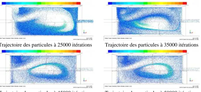
Pour tous les cas avec un débit massique d'entrée différent et une profondeur d'eau variable dans le réservoir, la ligne de trajectoire des particules est également différente. La structure du flux est le facteur principal qui affectera la ligne de trajectoire de la particule. La figure 12 illustre l’évolution de l’advection de particules dans un cas donné.
Trajectoire des particules à 3000 itérations Trajectoire des particules à 15000 itérations
Trajectoire des particules à 25000 itérations Trajectoire des particules à 35000 itérations
Trajectoire des particules à 45000 itérations Trajectoire des particules à 50000 itérations
Figure 12 Trajectoire des particules à 3 L/s
Le tableau 1 montre la comparaison de l'efficacité du décantation entre la simulation et l'expérience, dans les cas où le débit massique d'entrée est faible, la prédiction de l'efficacité du décantation est proche des résultats de l'expérience, mais la différence augmente pour des débits massiques d'entrée croissants.
Tableau 1 Comparaison de l'efficacité du décantation entre la simulation et l'expérience
Décharges d'entrée (L/s)
Profondeur d'eau (cm) Efficacité de décantation Simulation Expérience Simulation Expérience
1 11.48 8.3~8.6 77% 83% 1.5 11.98 12.0~12.2 74% 75% 2 12.37 13.2~13.4 70% 68% 2.5 13.35 14.5~14.9 72% 56% 3 14.49 14.7 64% 33% 3.5 15.91 14.9~15.2 53% 22% 4 17.39 15.8~16 56% 5%
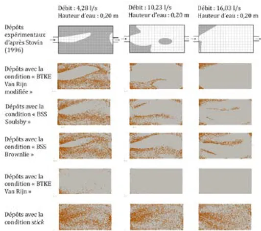
La figure 13 montre la comparaison des zones de dépôt entre la simulation numérique et les résultats de l'expérience à 3 L/s.
Figure 13 La comparaison des zones de dépôt entre la simulation numérique et les résultats de l'expérience à 3 L/s
La figure 14 montre la comparaison de la distribution du dépôt de sédiments dans le réservoir long avec cavité et sans cavité. L'existence de la cavité crée une partie qui favorise le piégeage des sédiments. La comparaison du résultat de la simulation numérique en utilisant la condition de décantation mise en œuvre et l'expérience montrent un bon accord dans la prédiction de la zone de dépôt, l'efficacité totale de piégeage du dispositif est comparable à celle mesurée expérimentalement.
Figure 14 La comparaison de la distribution du dépôt de sédiments dans le réservoir long avec cavité et sans cavité à 3 L/s
La condition de «piège» dans les codes d’écoulment n’est qu’une description très simplifiée des processus physiques réels en jeu lors de la sédimentation. Elle conduit à une forte surestimation de l'efficacité du piège et une prévision inexacte des zones de dépôt. Afin d’améliorer la prédiction de la sédimentation des particules, une fonction définie par l'utilisateur basée sur la courbe de shields a été implémentée pour la condition limite au fond.
La condition de limite améliorée est plus précise dans les conditions avec un débit liquide d'entrée faible que pour des débits élevés. La raison en est que le mouvement des particules devient plus compliqué en raison de l'augmentation du débit liquide d'entrée conduisant à un écoulement plus turbulent. Des phénomènes de resuspension, non pris en compte, peuvent également avoir lieu.
La simulation du transport des sédiments la bassin court ST montre que le centre de la zone de dépôt est retrusif et l'incertitude mesurée le long de l’axe des X est beaucoup plus élevée que celle mesurée selon Y. Et la distribution du diamètre des particules déposées est du même type, bien que le débit d'entrée change.
Le processus de transport des sédiments est un processus aléatoire. Théoriquement, le critère de dépôt et de début de mouvement n'est pas le seul paramètre qui déterminera l'état de la particule. L'introduction de la méthode stochastique au critère pourrait être une idée utile pour améliorer la prédiction de l'efficacité de dépôt et de la zone de dépôt des sédiments.
Les particules déposées forment la nouvelle limite, la différence entre le lit des particules et le lit du réservoir signifie le changement des conditions de décantation, ce qui pourrait conduire à une mauvaise prédiction dans la simulation numérique.
Travaux expérimentaux
Le dispositif expérimental, utilisé dans le cadre de cette thèse, est représenté par la Figure 15. Le dispositif de mesure (transducteur) est basé sur l'analyse d’un signal ultrason rétrodiffusé par un nuage de particules. Le transducteur de mesure est fixé dans un support mobile sur le réservoir expérimental. Il peut se déplacer dans le sens de la longueur et le sens de la largeur du réservoir. L’eau pompée d’un réservoir de stockage est déversée dans le bassin expérimental. Les particules injectées dans le bassin sont mélangées dans l’unité d'injection. L'eau chargée de particules est déversée dans le bassin collecteur. les particules déversées sont colléctées en utilisant un filtre disposé en sortie de bassin.. le niveau d'eau dans le bassin expérimental est contrôlé par une vanne de réglage située à l’aval du bassin.
Figure 15 Schéma du dispositif expérimental
Pour chaque débit d'entrée, nous fixons 60 positions de mesure dans le réservoir, réparties sur toute la section du réservoir de telle sorte à construire des champs de vitesses représentatifs des écoulements crées.
Les expériences sont réalisées pour des niveaux d’eau faibles et des niveaux d’eau élevés. Il existe deux types de profil de vitesse verticale. Le premier est la répartition de la composante de la vitesse dans la direction X (sens de l'écoulement) dans le plan vertical, le plan est positionné à 0,3 m de l'entrée dans le sens de l'écoulement. Le second est la répartition de la composante de la vitesse dans la direction X selon la position Z des lignes verticales. Toutes les lignes sont positionnées à 0.3 m, 0.6 m, 0.9 m, 1.2 m, 1.5 m, 1.6 m, 1.7 m, 1.8 m, 2.1 m, 2.4 m, 2.7 m and 3 m de l'entrée du bassin.
Figure 16 Profil vertical de la composante de la vitesse dans la direction de l’écoulement à X = 0,3 m pour un débit de 1 L/s à faible niveau d'eau
Figure 17 Distributions verticales de la vitesse (X= 0.3m-1.2m) pour un débit de
1 L/s
Figure 18 Distributions verticales de la vitesse (X = 1.5m-1.8m) pour un débit de
1 L/s
Figure 19 Distributions verticales de la vitesse (X = 2.1m-3m) pour un débit de 1
L/s
Le tableau 2 montre l'efficacité de dépôt dans différentes parties du réservoir, pour différentes conditions d'écoulement.
Tableau 2 Efficacités de sépôt dans différentes parties du réservoir. Débits d'entrée (L/s) Profondeur d'eau (cm) Efficacités de dépôts
Avant Cavité Arrière Total 1 11.8 60.16 % 30 % 9.85 % 100 % 1.5 12.5 25.84 % 44.1 % 29.56 % 99.5 % 2 12.5 16.97 % 38.48 % 42.22 % 97.67 % 2.5 12.5 8.58 % 17.58 % 56.14 % 82.3 % 3 12.5 2.63 % 11.48 % 41.92 % 56.03 % 3.5 12.6 7.91 % 2.76 % 31.78 % 42.45 % 4 13 1.75 % 1.06 % 18.83 % 21.64 % 15
4.5 13.5 1.2 % 0.3 % 0.5 % 1.8 %
Figure 20 Efficacité de dépôt dans différentes parties du réservoir
L'efficacité totale de dépôt diminue quand le débit d'entrée augmente. Lorsque le débit est supérieur à 4.5 L/s, l'efficacité de dépôt est proche de 0. Une expérience démonstrative a montré que pour un débit de 5 L/s aucune particule injectée ne s’est déposée dans le réservoir. En général, l'efficacité de dépôt a tendance à diminuer avec l’augmentation du débit d’entrée dans les trois parties explorées du réservoir (avant, cavité et arrière).. Dans le cas où le débit est supérieur à 2 L/s, l'efficacité de dépôt dans la partie avant diminue de 10%. On observe une augmentation rapide de l'efficacité de dépôt dans la cavité lorsque le débit passe de 1 L/s à 1.5 L/s. Ensuite, l'efficacité de dépôt diminue en continu avec l'augmentation du débit,. L'efficacité du A l’arrière du réservoir, l'efficacité de dépôt augmente quand le débit varie de 1 L/s à 2.5 L/s puis diminue à partir de 2.5 L/s.
Par comparaison à la simulation numérique, l'expérience peut montrer beaucoup plus d'informations. La distribution de la vitesse verticale peut être divisée en deux types: la première est la zone proche du flux d'injection où la vitesse verticale augmente du fond vers le centre d'injection jusqu'à un pic puis diminue de l'injection centrale à la surface libre. La seconde est la zone éloignée de l'injection de flux, la vitesse verticale est plus uniforme. La structure de l'écoulement dans le cas où la profondeur de l'eau est inférieure à 13 cm est principalement dominée par deux tourbillons, où un
tourbillon est dans le coin près de l'entrée et l'autre est grand et étalé vers l'aval, le débit d'entrée peut modifier l'écart de L'injection du flux. La structure de l’écoulement dans le cas où la profondeur de l'eau est supérieure à 13 cm est également constituée par deux tourbillons, mais ces deux tourbillons sont principalement situés dans la partie amont de la cavité. A l'aval l’écoulement est uniforme.
La cavité présente de meilleures performances dans le piégeage des sédiments lorsque le débit d'entrée est inférieur à 3.0 L/s, avec un débit d'entrée plus élevé, l'efficacité de dépôt est assez faible. La profondeur de l'eau dans le réservoir rectangulaire est un facteur important pour l'efficacité de dépôt, en général, l'efficacité est beaucoup plus élevée avec une profondeur d'eau plus élevée dans le réservoir.
Mots clés: écoulements, transport de sédiments, simulation numérique, expérience, efficacité de dépôt, réservoir, cavité, système d'eaux pluviales.
Acknowledgements
Firstly, I want to express my sincere gratitude to my supervisors, Professor Abdallah Ghenaim and Associate Professor Abdelali Terfous for the attentive and diligent guide to my PhD investigation. In the past three and half years, Abdallah Ghenaim gave his support on the subject in the numerical simulation and especially the experimental measurements, Abdelali Terfous gave his guidance in the progress of this research, I’m really thankful to his advice and encouragement in the discussion.
I’m also grateful to Pierre-André Garambois , who put forward plenty of useful advices in my numerical simulation and his patience and conscientiousness in the modification of my manuscript.
I would like to thank Pierre François for his accompany and patient guidance in my experiment work, and also for his help on dealing with the raw experimental data. I also want to thank all the members in the laboratory for their support during all my PhD career, and the help from the technician in INSA de Strasbourg and IMFS really means a lot in my experiment work.
I’m really grateful to China Scholarship Council for the financial supporting in the past three and half years, also I’d like to thank INSA de Strasbourg for providing me a wonderful research place.
At last not the least, I want to express my gratitude to my family, especially my father, my mother, my old sister and my brother in law, for their selfless support on my study career.
Table of contents
Acknowledgements ... 18
Table of contents ... 19
General introduction ... 22
1. Literature review ... 29
1.1 Characteristic of sediment and stormwater system ... 29
1.1.1 General description of sediment ... 29
1.1.2 Sediment in sewers ... 34
1.1.2.1 Sources of the sediment ... 35
1.1.2.2 Function of sedimentation tank ... 36
1.2 Mechanism of sediment transport ... 38
1.2.1 General ... 40
1.2.2 Suspended load ... 41
1.2.3 Incipient motion of sediment ... 42
1.2.3.1 Incipient drag force ... 42
1.2.3.2 Shields’s incipient curve ... 44
1.2.3.3 Initiation of suspension ... 46
1.2.3.4 Incipient velocity ... 48
1.2.4 Deposition ... 49
1.3 Research works on flow and sediment transport in tank ... 50
1.3.1 A summary of sediment transport modeling ... 50
1.3.2 Experiment works on flow and sediment transport in tank ... 54
1.3.3 Numerical simulations on flow and sediment transport in tank ... 56
1.4 Conclusions ... 64
2. Simulation of flow patterns in storm tank ... 66
2.1 Introduction ... 66
2.2 Numerical method ... 66
2.2.1 Flow governing equations ... 66
2.2.2 Discretization of the governing equations ... 68
2.2.3 Turbulence model ... 69 19
2.2.4 Boundary condition... 74 2.2.4.1 Inlet ... 74 2.2.4.2 Outlet ... 74 2.2.4.3 Free surface ... 74 2.2.4.4 Wall ... 75 2.3 Simulation setup ... 78
2.3.1 Geometry and mesh ... 78
2.3.2 Mesh sensitivity ... 80
2.4 Simulation results of the short tank ... 82
2.4.1 Water level ... 82
2.4.2 Flow pattern ... 83
2.4.3 Wall shear stress and turbulent kinetic energy ... 87
2.4.4 Velocity ... 90
2.5 Simulation results of the long tank ... 92
2.5.1 Water level ... 93
2.5.2 Flow pattern ... 93
2.5.3 Wall shear stress and turbulent kinetic energy ... 98
2.5.4 Velocity ... 101
2.6 Simulation results of the long tank with cavity ... 104
2.6.1 Water level ... 104
2.6.2 Flow pattern ... 104
2.6.3 Wall shear stress and turbulent kinetic energy ... 109
2.6.4 Velocity ... 112
2.7 Conclusions ... 114
3. Simulation of sediment transport in rectangular reservoir ... 116
3.1 Introduction ... 116
3.2 Method for modelling sediment transport ... 117
3.2.1 Approaches for particle trajectory ... 117
3.2.2 Turbulence dispersion of particles ... 124
3.2.3 Discrete random walk model ... 126
3.2.4 Boundary condition... 128
3.2.5 Approaches for implementation of settling condition ... 131 20
3.3 Sediment transport with using the trap condition in steady state ... 132 3.4 Implementation of settling condition with bed shear stress ... 134 3.4.1 Suspension particle tracking ... 139 3.4.2 Particle deposition zone ... 145 3.4.3 Statistic analysis for the sedimentation ... 148 3.5 Conclusions ... 151 4. Experiment of flow patterns and sediment transport in storm tank with variable cavity ... 153 4.1 Introduction ... 153 4.2 Experiment devices ... 154 4.2.1 Geometry ... 154 4.2.2 Particle characteristic ... 158 4.2.2.1 Introduction ... 158 4.2.2.2 Description of the particles ... 159 4.2.2.3 Granulometric analysis for the particles ... 160 4.2.2.4 Measurements of the settling velocities of particles ... 162 4.3 Measurements of the velocity field ... 167 4.3.1 Vertical velocity profile ... 168 4.3.2 Horizontal velocity profile ... 172 4.4 Measurements of sediment transport ... 175 4.4.1 Cases of low water level ... 176 4.4.1.1 Photograph of the sediment distribution ... 176 4.4.1.2 Trap efficiency ... 181 4.4.2 Cases of high water level ... 183 4.4.2.1 Photograph of the sediment distribution ... 183 4.4.2.2 Trap efficiency ... 186 4.5 Comparison of numerical simulation and experimental results in sediment transport ... 188 4.6 Conclusions ... 191 General conclusions ... 193 Numerical simulation ... 193 Experiment investigation ... 194 Perspectives ... 195 References ... 197 21
General introduction
Since the 4th century in Rome, the sediment problem becomes an issue that deserves to be attached importance to. As the sediment problem plays an important role in urban drainage system, which is in relation to the human daily life tightly, it will get more attention easily. Not only in the drainage system, sediment problem is also very common in the natural environment, rivers, seas or even in the air in the form of dust, smoke which leaves carbon spots on the wall or smog being a mixture of pollution and fog, as well as all chemical pollutants, all the process where the sediment problem is related prove the significance of the sediment problem without question. However, it is until the high development of urbanization that the sediment problem becomes more and more severe, which results in more and more attention being payed to by researchers and general public.
Stormwater management is one important part of the urbanization, in which the discharge runoff contains many kinds of pollutants, including nutrients, solids, metals, salt, pathogens, pesticides, hydrocarbon and so on. All the sediments discharged by stormwater runoff can be conveyed to all the near natural water area and sewer system. According to the report of Massachusetts Department of Environment Protection (MDEP, 1997), the largest contributors to water quality problems in the Commonwealth's stream, rivers and marine waters is the discharge from stormwater drain pipes and stormwater runoff. With progressive urban development in recent decades, the convey abilities of drain and pipe system in urbanized catchments and natural waterways has been increased significantly in quantities, water flow and rate, which leads to the urban flooding in the end. Research has shown that there has been a growing global trend of flood over last decades within the context of global climate change.
In general, the problem caused by sediment is not only variable and also is closely linked to the human being. With the continuously development of urbanization, the problem caused by sediment become more and more serious and demand prompt solution. In recent decades, growing public awareness of sediment problem has significantly emphasized the importance of environmental management of sediment problem. As mentioned above, the damage caused by sediment problems is
tremendous grievous not only in economy and also in common security. Many investigators and researchers devote to the investigation of sediment problem. For more than two centuries, workers in the sediment field attempted to formulate the conditions of incipient motion of sediment. In decades, the sediment transport in channels are processed in many research programs. Yalin (1963,1972), Yang (1972, 1973) and Vanoni (1984) find the extension. In this century, more than 50% of the population lives in the city, the portion will be even higher in the developed countries. A well operational urban water system will be significant to the daily life of the people living in the city. The sediment problem in urban water system will lead to city flood and contamination to the related aquatic habitats. In UK, a vegetated sustainable urban drainage system (SuDS) are constructed for flood risk management purposes. Up to 85% of the contaminants in the urban drainage system are conveyed to the stormwater system by absorption to fine sediment. The damage of the sediment in urban water system can be generally concluded as acceleration of maturing of the pipe, blocking the pipe path and so on.
Figure 1: Bedload sediment accumulation in sewerage and near inlet to pond (Snowmass, CO)
As a typical representative of sediment problem, stormwater management has its own difficulty and complexity. The purpose of stormwater management is to collect, treat and (re-)use runoff water, to restore the disturbed urban water cycle and to avoid contamination and destruction. The portion of impervious surfaces such as roofs in urbanized area and pavement has been increased due to the process of urbanization, which also leads to the increase of sediment entering the stormwater runoff, beacause those impervious surface prevent precipitation from soaking into the ground directly. The increasing load of stormwater runoff enters into drainage ditches, storm drains and sewer system rapidly, which cause problem as follow: stream bank erosion, Infrastructure damage, downstream flooding, contaminated streams, rivers and coastal water, combined sewer overflow.
Figure 2: The purpose of stormwater management
Stormwater runoff can cause frequent flooding and contaminated natural water area by conveying the carrying contamination. The principle design for the stormwater management is identical, however the stormwater management varies depending on the local condition such as climate, topology and resources. Meanwhile, the stromwater management should vary depending on the age. Traditional stormwater management aims at collecting stormwater in pipe networks and transporting it off site safely, as for speed and economy, the method for stormwater management is to discharge the runoff to combined sewer systems flowing to a wastewater treatment
plant, or to rivers or streams, or to a large stormwater management infrastructure directly. However, the highly developing urbanization increases the quantities of stormwater runoff and alters the quality of the stormwater runoff, which is expected to convey to urban receiving waters. This variation makes traditional stormwater management hardly to fulfill the desire of general public to high quality of environment, which was designed to meet the community's need to minimize the threat of flood. So in the field of stormwater management, a need for not only greater information on managing the urban water cycle and additional design and assistance with implementation but also the quality of stormwater. Once the sediment enter the stormwater system, it will retain in the urban water system.
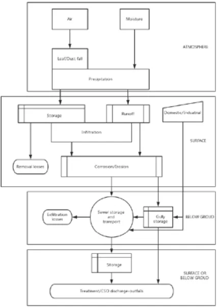
Figure 3: Pathways for sediment in urban water (Ashley, 2004)
The first approach used for stormwater management is detention/retention system, the main device is detention or retention basins or ponds. Originally, the detention basins were designed only for regulating the peak flow points. However, pollutant removal effect can be provided by the stormwater detention basins under the circumstance adequate settling time and sufficient size are available. Meanwhile, controlling discharge rate and reducing the flow velocity permit those facilities decrease the impact that urban development and impervious surface can have on water quality and aquatic habitats and reduce the possibilities of flood. Considering all those advantage the detention basins contain, more and more stormwater detention basins are used to control the quantity and quality of water. In 1970s, several researchers put forward an idea that using stormwater detention basins to fulfill dual purpose of mitigation of pollutant runoff load and flood control.
Though over past two decades the improvement in efficiencies of detention basins have been extensively discussed in the literature, both the basins designed for quantity and quality and the basins only for stormwater runoff peak discharge magnitude mitigation fail in perform the role to reduce stormwater runoff pollutant load. Usually the attention for detention basin is focused on increasing settling efficiency rather than limited possibilities in the removal of solid pollutant. Due to lack of enough acknowledge in pollutant particle transport and hydraulic characteristics of flow, the residence time of the detention basin is considered as the main way to evaluate the removal efficiency.
The dynamic nature of pollutant loads, the state of systems (temperature, water depth) and the entrance flow rate leads to the complexity of the stormwater detention system, however the detention basins are generally designed for the steady state. Nix et al (1985) stated that evaluating a stormwater detention system under steady state is inappropriate. Furthermore, it's hard to obtain the residence time of existing detention basins. Sediment characteristic and flow condition including residence time are main factor that can play influence on particle removal efficiency. Many experiment works and numerical simulations have been carried out on small scale model. Adamsson et al (2003) used a fixed bed shear stress boundary condition to model the sedimentation process. Dufresne carried out plenty of experiment to investigate the sediment transport. The experiment device used in the work of Dufresne was a simple rectangular tank, the dimension of which is 𝟏𝟏𝟖𝟖𝟎𝟎𝟎𝟎 𝒎𝒎𝒎𝒎 × 𝟕𝟕𝟕𝟕𝟎𝟎 𝒎𝒎𝒎𝒎 × 𝟒𝟒𝟎𝟎𝟎𝟎 𝒎𝒎𝒎𝒎, one cylinder pipe entrance and one cylinder pipe exit were included both with the diameter 80mm. Yan (2013) processed experimental work in a situ tank and run simulation of sediment transport in a small scale basin under steady and unsteady state, though improved the prediction of trap efficiency of the numerical simulation, the prediction of trap efficiency by numerical ways is still not satisfactory.
In general, there still exists problem in the simulation of sediment transport, the high prediction of trap efficiency and inaccurate prediction of spatial distribution of sedimentation zones. And the investigation on a simple rectangular tank can no longer fulfill the request of design of detention basin.
In this thesis, a new geometry is added to the bottom of a rectangular tank to investigate the effect of the new geometry on the flow and sedimentation. Also the research on how to use numerical simulation to model sediment transport is still necessary. Following works are finished:
• The numerical simulation of flow field is processed for three geometries, including short tank, long tank and long tank with cavity, where a volume of fluid model is applied to track the free-surface in the tank.
• The sediment transport in short tank and long tank with cavity is simulated by weak coupling of discrete phase and fluid calculation, a settling condition based on Shields diagram is implemented to the boundary condition.
• Velocity measurements of sediment transport in long tank with cavity are accomplished, the sediment deposition type in two water level is recorded.
There are three main objectives of this thesis. The first one is to understand the flow patterns in a storm tank in the 3D dimension, and to figure out the flow patterns is sensitive to which parameter. The second is to provide an effective ways for modeling the trap efficiency and spatial distribution of particles in a storm tank. The third is to investigate the effect of a cavity in a rectangular tank on the flow and sediment transport.
To realize these objectives, we organize our work in 4 chapters with a general introduction and a general conclusion.
The general introduction illustrates the importance and feasibility of the investigation, as well as the goal to achieve.
Chapter 1 presents a detailed literature review on numerical simulation and experiment works on flow and sediment transport in stormwater management field, and also gives an illustration on sediment investigation, including sediment source. Chapter 2 presents the numerical simulation of flow patterns in rectangular tanks with different geometry, illustrates basic theory for the numerical method and the process of running a numerical simulation.
Chapter 3 processes the numerical simulation on the sediment transport, tests the default boundary condition in the Fluent codes and comes out a new boundary condition based on bed shear stress, and validates with experiment results.
Chapter 4 introduces the experiment works in the laboratory, the measurement mechanism is illustrated, the particle information is given, and the analysis of experiment results is shown.
The general conclusion presents all the results obtained in this thesis and point out the possibility for the future investigations.
1. Literature review
This chapter begins with a general description of sediment, the state of the sediment in the stormwater system and how to deal with the sediment problem in the sewer. Therefore, the theory for sediment transport process is been illustrated. In the end, numerical simulation and experiment works on sedimentation tanks by others researchers are presented.
1.1 Characteristic of sediment and stormwater
system
1.1.1 General description of sediment
Essentially, sediments are solid fragments which originate from erosion of rocks by the physical and chemical disintegration. With the differences of origination, mineral composition, size and physical and chemical characteristics, the process of scour, transport and sedimentation of particles will be extraordinarily diverse. As the existence of sediment, the flow should be disposed as liquid-solid two phase flow, which means the sediment properties will be very critical to investigate the problem of sedimentation.
Particle size and density are the most important physical property of the sediment particle. It has a direct effect on the mobility of the particle and can range from great boulders, which are rolled only by mountain torrents, to fine clays, which once stirred uptake days to settle. Normally, the physical characteristic description of sediment can be classified as describing the size, shape and density.
According to the size of particles the sediment can be classified as many types, see the figure as follows: Figure 1.1 shows the relations in phi sizes, millimeter diameters, size classifications, ASTM and Tyler sieve sizes. The relations corresponding intermediate diameters, grains per milligram, settling velocity and threshold velocity for traction are described.
Figure 1.1 Size classifications of sediment particles (Widera,2011)
The size of sediment varies from micrometer up to centimeter when they are put under the spectrum, which make it challenge by classified the type by size due to so many variable value. However, there exist other methods to classify, for example classify by the shape or density. And there still exists a popular method for classification, which is based on the electrochemical interaction between sediment particles, where all the sediment is divided into two main groups, which are cohesive and non-cohesive sediment. The cohesive sediment always exists in the form of mixture with very fine sediment, such as organic material, clay and silt. Due to the existence of electrochemical processes, cohesive particles always attract each other to form into large object, which is so called “flocs”. In a flow field, the behavior of flocs and small particles are different, the flow pattern will be influenced by the flocs in a different way with small particles in a same volume. Due to the interaction between flocs and flow, flocs will break into smaller flocs. The flow properties and the material properties of small particles are the two main factors that determine the strength and size of flocs. The cohesive sediment transport is very complicated due to the breaking and complex patterns of floc creation, up till now the investigation only processed to a limited extent. The non-cohesive sediments are defined as particles where the electrochemical interaction can be neglected, and these particles will not form into flocs due to the material they are made of, their own mass and inertia. Due to the complexity of cohesive sediment transport, the particle mentioned in sediment transport is non-cohesive sediment.
The sediment particle ranges from great boulders to fine clays, due to which the size difference would be more than million times, and that’s why method of measurement is not unique. To substance like sediment particle without regular shape, it’s not sufficient to just obtain the size, used measure method and definition of the results should be detailed. The nominal diameter refers to the diameter of a sphere of same volume as the particle, usually measured by the displaced volume of a submerged particle. The sieve method is the most convenient way to determine the size of particles from boulder to fine sand. The sieve diameter is the minimum length of the square sieve opening through which a particle will fall. To the particle smaller than fine sand, the only method is the fall method. The fall diameter is the diameter of an equivalent sphere of specific gravity δ= 2.65 having the same terminal settling velocity in water at 24°C.
Density is the most fundamental parameter and must be known. The particle density, 𝜌𝜌𝑠𝑠 , is defined as its mass per unit volume when it’s inseparable. The particle specific
weight, 𝛾𝛾𝑠𝑠, corresponds to the solid weight per unit volume. Also the specific weight, 𝛾𝛾𝑠𝑠 , equals the product of the mass density of a solid particle, 𝜌𝜌𝑠𝑠 , times the
gravitational accelerating, thus:
𝛾𝛾𝑠𝑠 = 𝜌𝜌𝑠𝑠⋅ 𝑔𝑔 (1.1)
Shape and roundness are other factors that do have an effect on sediment transport, though there is no direct quantitative way to measure shape, roundness and their effects. Generally, shape is the entire geometrical pattern of the particle and there are many modes to describe it. Wadell (1933) used sphericity to describe the shape, with the definition as follow:
𝛬𝛬 = 𝐴𝐴′/𝐴𝐴 (1.2)
Where, 𝛬𝛬 is the sphericity, 𝐴𝐴′ is the superficial area of the sphere with the same volume of the particle, 𝐴𝐴 is the superficial area of the particle. Current research has shown that the dynamic flow characteristic of two particles at the same sphericity would be identical practically.
Particle with different shape has different characteristics of transport and sedimentation. McNown (1951) suggested a shape factor 𝑆𝑆. 𝐹𝐹. = 𝑐𝑐/√𝑎𝑎𝑎𝑎 , where 𝑐𝑐 is the shortest of the three perpendicular axes (a,b,c) of the particle. The shape factor is always less than unity, and values of 0.7 are typical for naturally worn particles. Cailleux (1945) recommended a flatness elongation 𝐹𝐹. 𝐸𝐸. = (𝑎𝑎 + 𝑎𝑎)/2𝑐𝑐 .
Roundness is a parameter that represents the extent of blunt and tip of particle’s edge. Wadell (1933) defined roundness as:
𝛱𝛱 = (∑ 𝑟𝑟/𝑅𝑅𝑁𝑁𝑁𝑁 ) (1.3)
Where, 𝑅𝑅 is the maximal radius of the inscribed circle on the maximal projective plane, r is the curvature radius of each edge on the same plane, 𝑁𝑁 is the edge number of the particle.
In fact, it’s very complex to measure the roundness of a particle. Krumbein (1938)
calculated the roundness of some typical particles by the method of Wadell (1933) and made the results as figure, which could be treated as sample to decide the roundness of a specific particle. The actual application of this method had shown that it’s approximately the same through comparison between a specific particle and the figure and calculation from the method of Wadell. And it should be known that with
the reduction of particle size and curvature radius, the measure accuracy would be abated significantly.
Settling velocity is another important parameter for the particles. For the solid portion, the settlement of particles is mainly resulted from the function of gravity. The particle will reach a constant velocity under the influence of the gravity, which is named terminal velocity. When the drag equals the terminal velocity, i.e. difference of the solid and fluid velocities, 𝑣𝑣𝑠𝑠− 𝑣𝑣 = 𝑤𝑤 , following equation is obtained:
𝑤𝑤2 = 4 3 1 𝐶𝐶𝐷𝐷𝑔𝑔𝑔𝑔( 𝜌𝜌𝑠𝑠− 𝜌𝜌 𝜌𝜌 ) (1.4)
Where 𝐶𝐶𝐷𝐷 is the drag coefficient, 𝑔𝑔 is the particle diameter, 𝜌𝜌𝑠𝑠 and 𝜌𝜌 are the particle density and fluid density respectively and 𝑤𝑤 is the settling velocity.
Thus, if the drag coefficient 𝐶𝐶𝐷𝐷 is found, the problem of the particle in question is solved. For spherical particles of diameter d in a viscous fluid of dynamic viscosity , the drag coefficient can be defined. In laminar flow region, for 0.5 ≤ Re ≤ 1.0 , where 𝑅𝑅𝑅𝑅 = 𝑤𝑤𝑔𝑔/𝑣𝑣 , the Stokes' solution can be obtained:
𝐹𝐹𝐷𝐷 = 3𝜋𝜋𝜋𝜋𝑔𝑔𝑤𝑤 (1.5)
𝐶𝐶𝐷𝐷 =𝑅𝑅𝑅𝑅24 (1.6)
Under two circumstances, the particle is very small or the viscosity of the fluid is very large, the Stokes' solution can be considered. The inertia terms is completely neglected in solving the general differential equation of Navier-Stokes in Stokes' solution. The first person who have successfully included the inertia terms, at least partly to the solution of the Navier-Stokes equation seems to by Oseen (1927), and the solution can be expressed as:
𝐶𝐶𝐷𝐷 =𝑅𝑅𝑅𝑅 �1 +24 16 𝑅𝑅𝑅𝑅�3 (1.7)
A more complete solution for Oseen approximation provided by Goldstein (1929) can be formed as:
𝐶𝐶𝐷𝐷 = 24𝑅𝑅𝑅𝑅 �1 +16 𝑅𝑅𝑅𝑅 −3 1280 𝑅𝑅𝑅𝑅19 2 +20480 𝑅𝑅𝑅𝑅71 3 + ⋯ � (1.8)
Where 𝑅𝑅𝑅𝑅 ≤ 0.2
The level of the free stream turbulence rather than turbulence caused by the particle itself can strongly affect the value of drag coefficient. Also, whether or not the surface of the sphere is hydraulically smooth or rough can affect 𝐶𝐶𝐷𝐷 .
When 𝑅𝑅𝑅𝑅 ≤ 800, a formula suggested by Schiller and Naumann (1933) gives good results:
𝐶𝐶𝐷𝐷 = 24𝑅𝑅𝑅𝑅 (1 + 0.150𝑅𝑅𝑅𝑅0.687) (1.9)
Combined with the equation of fall velocity, Schiller and Naumann also derived another formula:
𝐶𝐶𝐷𝐷𝑅𝑅𝑅𝑅2 =43 𝑔𝑔𝜌𝜌𝑠𝑠𝜌𝜌− 𝜌𝜌𝑔𝑔 3
𝑣𝑣2
(1.10)
For ≤ 100 , Olson (1961) put forward another equation where the drag coefficient can be well represented, the equation is in the form as follows:
𝐶𝐶𝐷𝐷 = 𝑅𝑅𝑅𝑅 (1 + 3/16 𝑅𝑅𝑅𝑅)24 1
2 (1.11)
1.1.2 Sediment in sewers
It seems that stormwater system and sewer system operate separately, however the stormwater will run into the sewer and cause problems. The integrity of the sewer system often gets intervention from illegal stormwater connections. During rainfall events, the stormwater will infiltration into the sewer, which makes the discharge peak
point occur and the overflow design of sewerage starts to operate. Both the stormwater system and sewer system have the necessary in using the detention basin for the treatment of peak discharge and sediment problems.
1.1.2.1 Sources of the sediment
The presence of solids in sewers can cause a variety of problems. Since the first sewer system was built in Rome in the 4th century BC, there existed the problems caused by solids consequently. It was because of the advent of industrial society and urbanization, the problems became acute. Solids entering sewer systems originate from a variety of sources. Five main sources are defined as:
• the atmosphere
• the surface of the catchment
• domestic sewage
• the environment and processes inside the drainage/sewer system
• industrial and commercial effluents and solids from construction sites.
The presence of solids may cause a variety of problems to the sewers. However, many reported problems do not have sufficient evidence so that they are regarded as anecdotal.
The composition and concentration of sediment in the sewage system will be different depending on the location. Though the concentration of sanitary solids in sewage is widely reported in the standard texts, the location or representiveness of the sample is not normally specified(e.g. source, in sewer or at the sewage treatment works). Similarity, these are assumed to be mean values, representative of the whole flow. Table 1.1 shows some typical international values. In this table SS represents suspended solids, BOD5 is biochemical oxygen demand, COD means chemical
oxygen demand.
Table 1.1 Averaged reported pollutant concentration in domestic (Ashley,2004) Location SS h (mg/l) BOD5i (mg/l) COD j (mg/l) 𝑁𝑁𝐻𝐻3 ∙ 𝑁𝑁k (mg/l)
Abu Dhabi a 198 228 600 35 Brussels(Blegium) d 290 325 670 35 Brazil(NE) c 392 240 570 38 Denmark e 120-450 150-350 214-740 12-50 France f 150-500 100-400 300-1000 20-80 35
Germany g 325 300-500 600 40-100(total) Jordan a 900 770 1830 100 Kenya a 520 520 1120 33 USA b weak 100 110 250 12 medium 220 220 500 25 strong 350 400 1000 50 UK c 80-195 143 40-517 20-90 a
Horan (1990), b Metcalf and Eddy (1991), c Crabtree et al (1991), d Verbanck (1989), e Henze et al (1995), f Bertrand-Krajewski (1993), g averaged data from range of sources, h
1.1.2.2 Function of sedimentation tank
Sanitary system might be the closest way that contacts normal people to the sediment. With the development of urbanization both the quantity and quality of stormwater runoff delivered to urban water system have changed. In recent decades, people pay more and more attention to the pollutants, which is because of the importance of environment management of urban stormwater. As we all know, suspended solids and sediments are the main components of pollutants in sewer detention system, so the treatment of particles will become more and more important. Sedimentation is the last procedure before the effluent is discharged to the external, so it’s crucial to make sedimentation tank to work effectively.
It’s of great importance of sewage system in the process of urbanization, which also impels the treatment of sediment become more and more crucial. Sediments in the sewage system usually originates from five principal sources, which are atmosphere, the surface of the catchment, domestic sewage, the environment and processes inside the drainage/sewer system, industrial and commercial effluents and solids from construction sites. Without efficient management of those sediments unexpected result will happen, which may be very harmful to the environment and even to the human being.
Based on the purpose of collection, the sewer can be divided into combined, separate and above ground/underground sewer. Based on the purpose of transport, the sewer can be divided into gravity, pressure and vacuum sewer. In total, the type of the sewer system can be combined sewers, separate sewers, simplified sewers, solid free sewers, pressurised sewers, vacuum sewers and open channel drains. In those sewers, sedimentation tank can store water temporarily to regulate a flood.
The use of sediment tank is mainly for removing particles in the sanitary system. However the design of a sediment tank could not be obtained before it is constructed, which means the cost spent on constructing a tank will be wasted if the tank could not perform as it was supposed to be. With the development of computer science, it becomes possible to simulate flow in sediment tank with CFD codes, which is also called numerical computation.
There are two criterions for assessing the performance of sediment tank, one is the capacity of storage of water volume, the other is the maximum value of the pollution the tank can discharge. Flow condition in the sediment tank plays a very important role in the frame of mechanic fluid. As the fluid can not maintain a fix form independently, the flow conditions rely on not only the characteristics of the fluid and also the medium where the fluid move in.
Combined sewer overflow (CSO) control is recognized as a necessity (Ashley,2004). In France stormwater reservoirs serve many catchments, which is reported by Perez-Sauvagnat et al (1998) for the Seine st. Denis, by Faure et al (1998) for Nancy and by Charry and Lussagnet (1998) for Marseille. In Germany there are over 13,000 CSO control tanks working for the goal of capturing 80% of the settleable solids (Pitt, 2014). Detention-sedimentation basins are also widely used for water storage and improving the quality of the water. Table 1.2 shows the efficiency of detention basins and Table 1.3 shows the trap efficiency of detention basins in UK.
Table 1.2 Efficiency of detention basins (Nascimento, 1999)
Ulis Sud a detention basin Pollutant reduction after 2h of decantation(%) Yearly inflow load (kg/ha imp.) Yearly outflow load (kg/ha imp.) Yearly removal efficiency (kg/ha imp.) TSS 3902 387 90.1 88 BOD5 829 107 87.1 76 COD 2598 521 79.9 - TKN 189 91 51.8 - P total 44 22 50.6 - Pb 0.893 0.054 94 65 37
Zn 5.12 0.66 87.1 77
Cd 0.031 0.0051 83.7 -
Cu - - - 69
Hydrocarbons 65 4 94.2 -
Table 1.3 Trap efficiency of detention basins (Nascimento, 1999) Pollutants Imhoff settleability (24h) Detention basin 2h removal (%) Detention basin 6h removal (%) Range TSS 68 34 84 49-91 BOD5 32 13 48 14-53 Ptot 46 20 58 20-70 Pb 62 30 66 46-78 Oil/hydrocarbons 69 18 62 20-78 Total coliforms 71 60 72 47-73
1.2 Mechanism of sediment transport
The sediments problem involves with the mechanism of sediments eroding, transporting and depositing in the fluid, which happens in the nature world and human life frequently. Usually, the sediments problem could occur almost everywhere: in rivers, lakes, seas and hydraulic structures or even in the air. And sedimentation may always pertain to objects of various sizes, ranging from huge rocks to suspensions of fine particles. As indicated Yang et al (1996), there are many variables that affect the hydraulic of the flow and the nature of sediment transport in a natural stream. Unbelievable and extremely expensive example of sedimentation processes has happened in the whole world, which impels hydraulic researchers get knowledge about sediment transport. Sediment erosion, transport and deposition in fluvial system
are complex processes, however sediment and ancillary data are fundamental requirements for the proper management of river system, including the design of structures, the determination of aspects of stream behaviors, ascertaining the probable effect of removing an existing structure, estimation of bulk erosion, transport, and sediment delivery to the oceans, ascertaining the long-term usefulness of reservoirs and other public works, tracking movement of solid-phase contaminants, restoration of degraded or otherwise modified streams, and assistance in the calibration and validation of numerical models. Coarse material carried as bed load was focused on in the early study of sedimentation transport, other than suspended sediment. Bed load transport phase was better understood than the phase of suspension phase until 1925 when the problem of suspension was began to be dealt with. However, it's still not possible to predict the suspended-load discharge than bed load discharge with any greater certainty. For most engineering purposes, the study on sediment transport is to fulfill the certainty at a degree to predict the sediment discharge of an alluvial stream, which is still not possible though plenty volume of study was devoted to sedimentation mechanics.
In many situations sediment motion is of great importance. The estimated maximum flood level is a crucial factor to the cost of a flood control scheme, which in its turn may be seriously affected by the scour and subsequent downstream deposition of sediment, either temporarily during the course of a single flood, or as a part of a more permanent long-term process. The deposition of sediment may also reduce the storage capacity and therefore the value of reservoirs being used for some form of water supply. Similar deposition in harbors may require costly dredging or other measures for the continuous removal of banks and bars. Meanwhile, sediment also makes the environment contamination a critical social problem to the modern industrialization country. Pollutants discharged to the external environment from sewage system. According to Massachusettes Department of Environment Protection (MDEP,1997), stormwater runoff and the discharge from stormwater drain pipes were the largest contributors to water quality problems in the Common wealth’s rivers, streams, and marine waters.
Sediment transport with its attendant problems governs, therefore, a great many situations that are of major importance to civilized man. Indeed it is a major geological influence in the shaping of landforms, and the examples listed above are only short-term aspects of the long-term process. In dealing with these examples engineers are seeking to control this process(at least to a limited extent), and the task is formidable not only for its size but also for its complexity. In fact many features of sediment transport is still unkown, but progress continues to be made on the general problem by many investigator.
1.2.1 General
Usually referring to sediment transport, it means the motion of solid particles. The path of the sediment in the natural world can be concluded as erosion, transportation and sedimentation, which is presented in the Figure 3. In the natural world, this phenomenon is very common, and in the field of hydrology, water source engineering and hydraulic, it's a significant study object for the researchers. As mentioned in the general introduction, the problem caused by sediment transport can be severe and even expensive. Many experts start to investigate sediment transport since the awareness that sediment transport is in relation with a large variety of problems. A bed load equation with refinements and additions was developed by Yalin (1962, 1973), which is incorporating reasoning similar to Einstein (1942,1950).
Figure 1.2 Process of erosion, transportation and sedimentation (Julien,2010)
Sediment transport is a very complicated process, normally it will be classified as two main types roughly:
• suspended load transport, the suspended particles are transported as suspended load transport. The fine silt brought into suspension from the catchment area rather than from bed material load in suspended load is called wash load.
• bed load transport, usually the transport where particles is in rolling, sliding and saltating motion is called bed load transport. When the value of bed-shear velocity just exceeds the critical value for initiation of motion, the bed material particles start rolling and/or sliding in continuous contact with the bed. Saltation happens when continuing increasing the bed shear velocity.
Figure 1.3 Pattern of particle motion
In this work, what should be focused on is the suspension and the settling condition for the particle, hence the bed load transport is not the emphasis.
1.2.2 Suspended load
The suspended load transport will be expressed as the concentration C in mass (kg/m3) or in volume (m3/m3). A combination of convection, advection and turbulent diffusion can control the transport of suspended load. The advection-diffusion equation can be expressed as: 𝜕𝜕𝐶𝐶 𝜕𝜕𝜕𝜕 + 𝜕𝜕𝜕𝜕𝐶𝐶 𝜕𝜕𝜕𝜕 + 𝜕𝜕𝑣𝑣𝐶𝐶 𝜕𝜕𝜕𝜕 + 𝜕𝜕𝑤𝑤𝐶𝐶 𝜕𝜕𝜕𝜕 = 𝐷𝐷 �𝜕𝜕𝜕𝜕𝜕𝜕2𝐶𝐶2 +𝜕𝜕𝜕𝜕𝜕𝜕2𝐶𝐶2 +𝜕𝜕𝜕𝜕𝜕𝜕2𝐶𝐶2� + 𝜀𝜀𝑥𝑥𝜕𝜕 2𝐶𝐶 𝜕𝜕𝜕𝜕2 + 𝜀𝜀𝑦𝑦 𝜕𝜕2𝐶𝐶 𝜕𝜕𝜕𝜕2 + 𝜀𝜀𝑧𝑧 𝜕𝜕2𝐶𝐶 𝜕𝜕𝜕𝜕2 + 𝐶𝐶̇ (1.12)
Where D is the molecular diffusion coefficient and 𝐶𝐶̇ is the term of phase change source.
The suspension of particles are the result of increasing the flow velocity, the particle is taken into eddies moving up and the velocity component in the upward is larger than the settling velocity of the particle, at the meantime the size of the eddy is much bigger than the particle. After long time impact on the particle by eddies, the particle will enter the main flow. As a word, the suspension of the particle is the result of large
scale turbulence. In contrary, the suspended particle will decrease the intensity of the turbulence.
1.2.3 Incipient motion of sediment
By increasing flow intensity gradually, the bed sediment will start move from static, which is called incipient motion of sediment, the relative critical flow condition in which the hydrodynamic acting on the sediment reached an exact value putting the sediment in motion is called as initial condition of sediment. The force resisting the incipient motion depends on the size and the type of particle, for coarse particles, the force resisting the incipient motion should be the gravity, as for finer sediment, cohesion should be the main factor of resisting incipient motion. However due to the complexity of cohesion, which depends on the composition of sediment and the environment the particle located, until now very few knowledge is obtained about cohesion, thus almost all the researchers choose non-cohesive particle as study object. Determining critical condition for the sediment is of significant practice importance, an early work given by Lelliavsky (1955) reported a formula for critical velocity which was presented by Brahms (1753). Shear velocity and bed shear stress are two main parameter used popular for determine the critical condition.
1.2.3.1 Incipient drag force
In a uniform flow, the component in the flow direction of the drag force acted on the fluid per bed area can be expressed by:
𝜏𝜏0 = 𝛾𝛾ℎ𝐽𝐽 (1.13)
Where 𝛾𝛾 is the specific weight of the fluid, ℎ represents the water height and 𝐽𝐽 is the descending slope. This expression can be also used in the non-uniform flow only if 𝐽𝐽 is substituted by energy slope.
The dissipated energy by unit volume fluid per unit time can be formularized as: 𝑤𝑤𝑠𝑠 = 𝜏𝜏𝑔𝑔𝜕𝜕𝑔𝑔𝜕𝜕 (1.14)
If the water level is ℎ , the total dissipated energy by the unit width fluid per unit time will be : 𝑊𝑊0 = � 𝜏𝜏𝑔𝑔𝜕𝜕𝑔𝑔𝜕𝜕 𝑔𝑔𝜕𝜕 ℎ 0 (1.15)
The distribution of velocity along vertical direction can be expressed as:
𝜕𝜕 = 𝑈𝑈𝑈𝑈(𝜕𝜕) (1.16)
Where the mean vertical velocity 𝑈𝑈 = 1
ℎ∫ 𝑈𝑈𝑈𝑈(𝜕𝜕)𝑔𝑔𝜕𝜕 ℎ 0 . Therefore, 1 ℎ∫ 𝑈𝑈𝑈𝑈(𝜕𝜕)𝑔𝑔𝜕𝜕 ℎ 0 = 1.
In a 2D flow, the vertical distribution of shear is :
𝜏𝜏 = 𝜏𝜏0�1 − 𝜕𝜕 ℎ� �
(1.17)
Thus the total energy will be :
𝑊𝑊0 = � 𝜏𝜏0(1 − 𝜕𝜕 ℎ⁄ )𝑈𝑈𝑔𝑔𝑈𝑈(𝜕𝜕)𝑔𝑔𝜕𝜕 𝑔𝑔𝜕𝜕 ℎ 0 = 𝜏𝜏0𝑈𝑈 �� 𝑔𝑔𝑈𝑈(𝜕𝜕) 𝑔𝑔𝜕𝜕 𝑔𝑔𝜕𝜕 ℎ 0 − 1 ℎ � 𝑔𝑔𝑈𝑈(𝜕𝜕) 𝑔𝑔𝜕𝜕 𝑔𝑔𝜕𝜕 ℎ 0 � = 𝜏𝜏0𝑈𝑈 (1.18)
In addition, the energy slop of the flow Je physically equals to the dissipated energy of the fluid per unit weight in a distance per unit. Therefore, 𝑊𝑊0 can also be expressed as:
𝑊𝑊0 = 𝛾𝛾ℎ𝑈𝑈𝐽𝐽𝑒𝑒 (1.19)
1.2.3.2 Shields’s incipient curve
In 1936, Shields developed the incipient equation for uniform non-cohesive particles, based on the force balance exerted on the particle on the bed.The weight of a sphere particle is 𝑊𝑊′ = (𝛾𝛾𝑠𝑠 − 𝛾𝛾)𝜋𝜋𝐷𝐷3
6 , the main force acting on the particle from the flow are
drag force expressed as:
𝐹𝐹𝐷𝐷 = 𝐶𝐶𝐷𝐷𝑎𝑎1𝑔𝑔2𝛾𝛾𝜕𝜕0 2
2𝑔𝑔
(1.20)
And lift force expressed as:
𝐹𝐹𝐿𝐿 = 𝐶𝐶𝐿𝐿𝑎𝑎2𝑔𝑔2𝛾𝛾𝜕𝜕0 2
2𝑔𝑔
(1.21)
Where 𝐶𝐶𝐷𝐷 and 𝐶𝐶𝐿𝐿 are drag coefficient and uplift coefficient respectively, 𝜕𝜕0 is the flow velocity acting on the particle.
When the bed is constituted by uniform particle, the vertical velocity distribution has the form as follows:
𝜕𝜕
𝑈𝑈∗ = 5.75 log 30.2
𝜒𝜒𝜕𝜕 𝛼𝛼1𝑔𝑔
(1.22)
Where 𝛼𝛼1 is approximately around 2 and 𝜒𝜒 is relevant to particle Reynolds number 𝜒𝜒 = 𝑈𝑈1�𝑈𝑈𝜈𝜈∗𝑑𝑑�.
The 𝜕𝜕0 can be assigned as the velocity of 𝜕𝜕 = 𝛼𝛼2𝑔𝑔, where 𝛼𝛼2 is the coefficient near to 1.
Thus 𝜕𝜕0 = 5.75 𝑈𝑈∗log 30.2𝛼𝛼2
𝛼𝛼1𝜒𝜒 = 𝑈𝑈∗𝑈𝑈2�
𝑈𝑈∗𝑑𝑑
𝜈𝜈 �.
Then the critical condition of the particle starting slide is 𝐹𝐹𝐷𝐷 = 𝑈𝑈(𝑊𝑊′− 𝐹𝐹𝐿𝐿), where 𝑈𝑈 is the friction coefficient between the particles.