HAL Id: lirmm-00416221
https://hal-lirmm.ccsd.cnrs.fr/lirmm-00416221
Submitted on 13 Sep 2009
HAL is a multi-disciplinary open access
archive for the deposit and dissemination of
sci-entific research documents, whether they are
pub-lished or not. The documents may come from
teaching and research institutions in France or
abroad, or from public or private research centers.
L’archive ouverte pluridisciplinaire HAL, est
destinée au dépôt et à la diffusion de documents
scientifiques de niveau recherche, publiés ou non,
émanant des établissements d’enseignement et de
recherche français ou étrangers, des laboratoires
publics ou privés.
Seamless Joining Of Tiles Of Varying Resolutions For
Online 3D Terrain Visualization By Dwt Domain
Smoothing
Khizar Hayat, William Puech, Gilles Gesquière
To cite this version:
Khizar Hayat, William Puech, Gilles Gesquière. Seamless Joining Of Tiles Of Varying Resolutions For
Online 3D Terrain Visualization By Dwt Domain Smoothing. EUSIPCO: EUropean SIgnal Processing
COnference, Aug 2009, Glasgow, United Kingdom. pp.2112-2116. �lirmm-00416221�
SEAMLESS JOINING OF TILES OF VARYING RESOLUTIONS FOR ONLINE 3D
TERRAIN VISUALIZATION BY DWT DOMAIN SMOOTHING
Khizar Hayat
a, William Puech
aand Gilles Gesqui`ere
baLIRMM, UMR CNRS 5506, University of Montpellier II
161, rue Ada, 34392 MONTPELLIER CEDEX 05, FRANCE
bLSIS, UMR CNRS 6168, Aix- Marseille University
IUT, rue R. Follereau, BP 90178, 13637 ARLES CEDEX, FRANCE [email protected], [email protected], [email protected]
ABSTRACT
A novel context-based DWT domain smoothing strategy is being proposed for seamless tessellation of texture as well as the digital elevation model (DEM). In the use case, in per-spective, the tessellation is heterogeneous in resolution with three different tile qualities or levels of detail (LOD), at a given instant, depending on the viewpoint distance, the time of rendering and hardware resources. The LOD is dependent on the multiresolution characteristic of wavelets from the now widely accepted JPEG2000 codec. Three different join-ing functions have been employed to create subband-sized masks for each of the tile subbands selected for smoothing. The results, obtained for a practical example, have been in-teresting in the sense that it eliminated the popping artifacts to a considerable extent without affecting the field of view at a given instant.
1. INTRODUCTION
The technology is advancing by leaps and bounds, but it is still away too far from catching up with the ever increasing rendering throughput of terrain visualization. The problem is exacerbated when the data is to be transferred over some net-work, especially in a client/sever environment. With it comes another dimension in the shape of the client diversity in terms of memory, processing and bandwidth resources. For ex-ample, today’s geo-browsers, like Google Earth or NASA’s World Wind, do not take into account individual client char-acteristics and what one observes are lags and freezes for clients with low resources. All these factors necessitates some scalable data processing/structuring and the obvious choice is to create multiple levels of detail (LOD) by rep-resenting the shape at different levels of approximation. This is essential for the terrain tessellation adjustment as a func-tion of the view parameters [1]. For LOD one can rely on the multiresolution nature of the discrete wavelet transform (DWT). It is better to employ some standard state-of-the-art DWT, like the now widely accepted JPEG2000 standard1.
Additional advantages of the JPEG2000 could be good com-pression and capability to transfer the data progressively.
As far as the rendering of large terrains is concerned, tile-based approaches have always been a preference. Our strategy is to render a texture/depth map tessellation from JPEG2000-coded tiles wherein only visible tiles are rendered and the focused ones, out of these, have the highest quality depending on the viewer’s distance. As the viewer moves in, the tiles corresponding to the new view must be rendered at
1The ISO/IEC 15444-1 standard
and gradually refined in quality as the focus is coming near to it. This refinement is additive as more and more subbands are added to it, at runtime. The main challenge to this strategy is that the tile must be seamlessly stitched for both the texture and the digital elevation model (DEM) and the boundaries must be diluted enough to prevent popping artifacts. This phenomenon is observable even in the case of modern geo-browsers. While there have been many works on the seam-less rendering of DEM, the efforts focusing on the textures are far less. In this paper, although we are more inclined to the texture, the DEM has also been treated as its integral part. In fact this work is a continuation of our earlier efforts about the synchronous unification of the DEM/texture pair through data hiding [2].
Our strategy is aimed at context-based smoothing of the tile boundaries. The smoothing is carried out at the subband level in the DWT domain by employing various smoothing masks. The lowest resolution tiles of the panorama are not treated while the mid-level resolution and the highest resolu-tion tiles are modified to join them together. All this is ex-plained in Section 3 after a brief account of the background literature in Section 2. We applied our strategy to a practical worst case example and the results are shown in Section 4 which is followed by the concluding remarks in Section 5.
2. BACKGROUND
Terrain LOD algorithms can be classified [1], on the basis of the hierarchical structure, into four groups, namely the triangulated irregular networks (TIN), bin-tree hierarchies, bin-tree regions and tiled blocks. The tessellation, in the last category, is carried out with the square tiles of different res-olutions as has been done by Wagner [3]. But the process requires seamless stitching at the boundaries. According to Deb et al [4] the view frustum culling technique of [3] is not suited for the terrains with large height variations. They tweak the technique by having the projection on realtime av-erage height of terrain for a client/server terrain streaming to handle heterogeneous clients. The blending factors are cal-culated on a per tile basis because of the use of a regular tile structure, thus, reducing the amount of computation. Special techniques based on mipmaps and clipmaps can be found in the literature. According to [5], ”a mipmap is a collection of correlated images of increasingly reduced resolution ar-ranged, in spirit, as a resolution pyramid whereas a clipmap is an updatable representation of a partial mipmap, in which each level has been clipped to a specified maximum size”. Lossasso et al [1] breaks the terrains into geometric clipmaps of varying metric sizes which can be used as LODs through a
lirmm-00416221, version 1 - 13 Sep 2009
view-centered hierarchy resulting in a simplified spatial and temporal inter-level continuity.
A thresholding scheme based on calculated ground sam-ple distances is proposed in [6] with a nested LOD system for efficient seamless visualization of large datasets. In or-der to remove the T-junctions they have put forward a mesh refinement algorithm.Ueng and Chuang [7] propose a dike structure between two adjacent blocks, for a smooth blend-ing between two meshes of different LOD. This approach is combined in [8] with heuristics to dynamically stitch the tile meshes together seamlessly. For the texture part they use high resolution aerial photos subjected to the similar LOD mechanism as described for the meshes. Larsen and Chris-tensen [9] try to avoid popping for low-end users by exploit-ing the low-level hardware programmability in order to main-tain interactive frame-rates. They claim their work as pio-neering as far as a ’smooth’ LOD implementation in com-modity hardware is concerned.
Little attention has been paid to the texture images which require their own LOD structure. There have been propos-als, like texture clipmaps [5], but texture tiling is usually preferred. The multiresolution technique, described in [10], presents static LOD terrain models, allowing for combination of multiple large scale textures of different size. The view-dependent texture management technique in [11] manages multiresolution textures in multiple caching levels - database, main memory and graphics card memory - which the authors claim to be suitable for hardware with limited resources. The approach of [12] includes dynamic texture loading for mem-ory management and, combine several textures into atlases for avoiding too much texture switches [13]. Their compu-tationally complex preprocessing part helps them to signifi-cantly reduce runtime rendering overhead.
3. THE SMOOTHING STRATEGY 3.1 Scenario
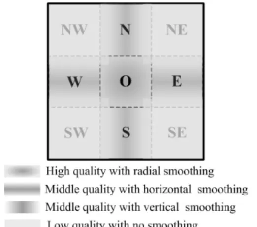
We are supposing a simplistic scenario of a panorama of 3×3 tiles. This use case will represent almost all the possibilities we will have in our application. An individual tile is large enough to circumscribe the field of view even if the observer is too far. In other words one can say that if the observer is too far, his/her view is limited to a 3 × 3 tessellation at maxi-mum with all the tiles at their lowest resolutions but as soon as he/she draws closer, further detail is added to the tile of focus to improve its resolution. The smoothing process will be done only on a 3 × 3 tiles. The rest of the encompassing tiles are in the low resolution and hence there is no need to smooth them. The tessellation is heterogeneous in terms of resolution and a given tile can have one of the three quali-ties, namely high middle and low. The high quality resolu-tion corresponds to the center which is the viewpoint focus. We are rendering the corners with low resolution and the 4-neighbors of the center with the middle resolution tiles. The terms high, low and middle are not static and their extent depends on the distance of observer from the view as well as the the time passed after the viewer changed his position. We are assuming this three quality environment because it reflects most of the possible cases in our application. Thus the 3 × 3 tessellation is not binding; rather it represents a simplistic worst-case scenario wherein three different qual-ity tiles can be seamlessly rendered. There may be a tessel-lation having concentric square rings with each successive ring having a different quality [5] but we believe that at any
instant one would hardly be dealing with a rendering involv-ing more than three resolutions. That is to say, our resolution set may contain a wide spectrum of resolutions but at a given time three of them would be rendered.
3.2 Viewpoint analysis
Our strategy is aimed at the seamless 3D visualization as a function of the network connection and the computing re-sources of the client. The resolution of various tiles in the tessellation is a function of its distance D between the ob-server and his/her focus on the terrain. As far as DEM is concerned, its quality is evaluated with the root mean square error (RMSE) in length units. As pointed out in some re-cently published works [14], even today the acquisition of the DEM, for 3D terrain visualization, is error prone and it is difficult to get a RMSE less than 1 meter in elevation. To calculate the maximum acceptable RMSE, for an optimal 3D visualization, we rely on the distance D (Fig. 1) and the vi-sual acuity (VA) of the human vivi-sual system (HVS). Vivi-sual acuity is the spatial resolving capacity of the HVS. It may be thought of as the ability of the eye to see fine details. There are various ways to measure and specify visual acu-ity, depending on the type of acuity task used. VA is limited by diffraction, aberrations and photoreceptor density in the eye [15]. In this paper we assume for the HVS that the VA corresponds to an arc θVAof 1 minute (10= 1/60◦). Then for
a distance D we have a focus of diameter 2 × D × tan(θVA) or
more simplistically E = 2 × D × tan(θ /2). Usually the field of view of the HVS is θ = 60◦. For example if E = 3200 m then D = 2771.28 m. For the 3D visualization, we should
Figure 1: Visualization of a depth map from a viewpoint. take into account of the resolution of the screen in pixels. As illustrated in Fig. 1, if we have an image or a screen with p pixels for each row, then the tolerable LOD error (ε) in p is:
ε = E/2
tan(θ /2)× tan(θ /p). (1) With θ = 60◦, E = 3200 m and a resolution of 320 pix-els, a PDA for instance, we have ε = 9.07 m. Then, in this context, for our application we can assume that a RMSE of about 9 m is acceptable for the visualization. Notice that we generate a conservative bound by placing an error of the maximum size as close to the viewer as possible with an or-thogonal projection of the viewpoint on the depth map. We also assume that the range data model is globally flat and that the accuracy between the center and the border of the depth map is the same. In reality, the analysis should be different and part of the border should be cut as explained by [16] in a
particular case of a cylinder. Anyhow, the value of D would help us to reach a decision about the resolutions of various tiles in the tessellation.
3.3 The Level of Detail (LOD)
For the LOD we are relying on the multiresolution nature of DWT from the JPEG2000 codec. The reasons for choosing JPEG2000 are its scalability, its wide acceptance as a stan-dard, its support to various wavelet forms for multiresolution, progressive transfer capability and last but not the least is its approximation paradigm for LOD. The various approxima-tions do not differ in size but only in quality which is additive in nature. If each tile is DWTed in the JPEG2000 codec at level L then a level-l (≤ L) approximate image is the one that is constructed with (1/4l) × 100 percent of the total coeffi-cients. These coefficients correspond to the available lowest 3(L − l) + 1 subbands and for the coefficients corresponding to the rest of the 3l subbands, zeros are stuffed. Subsequent application of L-level inverse DWT yields what is known as the l-approximate image. For example, level-0 approximate image is constructed from all the coefficients and level-2 ap-proximate image is constructed from 6.12% of the count of the initial coefficients.
3.4 Smoothing functions
Let the high, the middle and the low resolution of our sce-nario correspond to lh, lm and ll approximate images,
re-spectively. The quality gap would essentially bring with it the popping artifacts at tile boundaries. To undo that, we are proposing a wavelet-domain context dependent smooth-ing strategy graphically explained in Fig. 2. At the corners (NW, NE, SW and SE) are the ll-approximate images ob-tained from lowest 3(L − ll) + 1 subbands with the rest of 3ll subbands being replaced by 0s. For the rest of the tiles
one can partition their subbands into three sets. One, the lowest 3(L − ll) + 1 subbands will remain untouched since
they represent the lowest rendered quality. Two, the high-est 3lhsubbands of center tile (O) and 3lm subbands of its
4-neighbors (E,W,N and S) are stuffed with 0s. Three, the remaining 3(ll− lh) and 3(ll− lm) subbands of central tile
and its 4-neighbors, respectively. It is this third set (or its subset thereof) which will be subjected to the DWT domain treatment with three different smoothing functions on each subband individually:
1. for the left/right neighbors (W and E) of center use the horizontal smoothing function,
2. for the above/below neighbors (N and S) of center use the vertical smoothing function,
3. for the center (O) use the radial smoothing function. Note that we are affecting the quality of only a small part on the periphery of the tile during a given smoothing pro-cess. For any given subband, the smoothing function creates a scalar multiplication mask (over [0, 1]) of the size of the subband. The horizontal smoothing mask would have a cen-tral band of rows of 1’s. The thickness of this band depends on the maximum diameter, δ , of the view focus. If the sub-band belongs to the kth resolution level, then the thickness should be around δ /2k. Beyond the band of 1’s the rows gradually attenuate on both sides approaching 0 at the pe-riphery. Our horizontal smoothing function is described here in the form of algorithm 1. Along similar lines we can get a vertical smoothing mask which is nothing but a transpose of
Figure 2: The Tessellation Scenario
Input: width(w) of a DWT domain square subband Output: Horizontal w × w smoothing mask begin 1 δ ←− w/2; 2 min coe f f←− 0; 3
Initialize a vector B of size w ∗ w to 1.0;
4
for j = 0 to w/2 − δ /2 do
5
min coe f f←− min coe f f + 2/(h − δ );
6
for i = 0 to w do
7
B[i + w ∗ j] ←− min coe f f ;
8 end 9 end 10 for i = 0 to w ∗ w/2 do 11 B[w ∗ w − 1 − i] ←− B[i]; 12 end 13 return B; 14 end 15
Algorithm 1: Horizontal Smoothing Function
the horizontal mask for a given subband. The radial smooth-ing mask is a bit tricky. We would have a center core of 1’s having a diameter of about δ /2kfor a the subband of the kth resolution level. The shape of this core is more or less cir-cular – octagonal, to be precise. Each ring of coefficients around the core would gradually attenuate approaching 0 at the corners and around 0.5 in the up/down and left/right di-rections. Algorithm 2 is the logical representation of our ra-dial smoothing. After the smoothing treatment of a subset or all of the third group of subbands and inverse DWT one can have a seamless visualization of the type given in Fig. 2. In our application, we are using the same strategy for the DEM to avoid popping effect on elevation data.
4. RESULTS
We have applied our smoothing strategy to a practical ex-ample of 3072 × 3072 texture tessellation composed of 9 tiles of size 1024 × 1024. The corresponding DEM tessel-lation at our disposal has a size of 96 × 96 with each of the nine tiles having 32 × 32 coefficients. The texture tiles were transformed at level-4 reversible DWT in a standard JPEG2000 encoder whereas the DEM tiles were subjected to reversible level-4 DWT simply. In our example visualization,
(a) The original without smoothing (b) zoomed square of (a) (c) Full panorama with dm= 0, dh= 1 (d) zoomed area of (c)
Figure 3: Example Texture Tessellation: lh= 0,lm= 2,ll= 4
Input: width(w) of a DWT domain square subband Output: Radial smoothing square mask of width w BEGIN 1 δ ←− w/2; 2 interval←− 2/w; 3 w←− w/2; 4 for i = w ∗ h − 1 to 0 do 5 if i >= w ∗ (w − δ /2) then 6 if i%w >= (w − δ /2) then 7 temp[i] ←− 1.0; 8 else 9
temp[i] ←− temp[i + 1] − interval;
10
end
11
else
12
temp[i] ←− temp[i + w] − interval;
13 end 14 end 15 w←− w ∗ 2; 16 for i = 0 to w ∗ w/2 do 17 if i%w < w/2 then 18
B[i] ←− temp[i% bw/2c + bi/wc ∗ bw/2c];
19
else
20
B[i] ←− B[i − (2 ∗ (i% bw/2c) + 1)];
21 end 22 B[w ∗ w − 1 − i] ←− B[i]; 23 end 24 return B; 25 END 26
Algorithm 2: Radial Smoothing Function
we are going for the worst case for the corners by render-ing level-4 approximate tiles which would mean a renderrender-ing with only 0.4% of the coefficients. For the centre we are tak-ing highest possible quality, i.e. level-0. The 4-neighbors of center have the middle quality of level-2 approximation. The high quality gap between the three qualities is likely to make the tile boundaries conspicuous. A texture tessellation with these tiles without any smoothing treatment is shown in Fig. 3.a. The boundaries are not that visible due to the fact that the space we are using to render a large image of 3072 × 3072 pixels is too small. For this purpose we have magnified a small area (corresponding to the small square in Fig. 3.a) from the tessellation in Fig. 3.b. We have deliber-ately selected a region that contains each of the resolution
and smooth quality. This magnification is only for a compar-ison and the magnified portion does not represent the visual effect we are upto since the distance it represents warrants improved qualities at corners in our strategy. We will not be showing the whole tessellation for the treated examples but rather displaying the corresponding square region in each tessellation for comparison. Let d implies that 3d + 1 lowest subbands have been avoided during smoothing, e.g. d = 1 implies that the lowest 4 subbands have not been touched. Based on d we are defining dhwhich corresponds to the
cen-ter tile and dmthat corresponds to the 4-neighbors. Note that
since the 4-neighbors are level-2 approximates, the highest six subbands are already zero. This implies that dm cannot
exceed 1. If we do not tamper the lowest four subbands dur-ing the horizontal smoothdur-ing of E/W and vertical smoothdur-ing of N/W then dm= 1, otherwise dm= 0 where the only lowest
level-4 subband is avoided from smoothing. dh, which
cor-responds to the center O, can assume a value of up to 3 and it was observed that the border between the four tiles gradu-ally smoothen as we decrease the value of dhsince more and
more subbands are being involved in the radial smoothing of O. Since we are working on a worst case scenario and we are closer than we should be, the borders do not disappear at all but in the original environment the transition is seamless. Due to space constraint we are showing only one example smoothing in Fig. 3.c, where dl= 0 and dh= 1. Its
magni-fied part corresponding to Fig. 3.b is illustrated in Fig. 3.d. From the latter, it can be observed that the border between the four tiles is far more smoother than the original.
Along the same lines the DEM can also be treated but the ex-ample at our disposal has a 96 × 96 DEM for a panorama of 3072 × 3072 which we believe is too small to be efficiently decomposed. It would have been interesting to take into ac-count a larger DEM but due to circumstances beyond our control we were compelled to use a smaller DEM. Nowadays the DEM resolutions are approaching those of textures and hence for such DEMs one can safely apply the smoothing. A 3D visualization realized from a subset portion, at a partic-ular angle, of the original example and one of the smoothed version, with dl= 0 and dh= 1, are illustrated in Fig. 4. A
3D view with the original can be seen in Fig. 4.a., marked by red ovals for the sake of comparison. Fig. 4.b shows the 3D view of our smoothed example and a comparison of the areas inside the red ovals with those in Fig. 4.a. suggests that the borders between the tiles are more diluted in the former case.
(a) No smoothing
(b) Smoothing: dm= 1, dh= 3
Figure 4: A 3D view corresponding to Fig. 3. 5. CONCLUSION
The results have been interesting in the face of the fact that we presented a worst case example tessellation in terms of quality difference as well as DEM size. The question arises that if the DEM is different enough to warrant its own LOD, how can one synchronize it? The answer to this is the fact that since the LOD is wavelet driven, one can always syn-chronously unify the DEM texture pairs as explained in [2] or even adapt the synchronization [17] to exclude some sub-bands from embedding. In the continuation of our work we would like to add some other techniques to our strategy, the foremost being mosaicking. We believe that if we mix up our smoothing strategy with DWT domain blending of sub-bands in adjacent heterogeneous tiles, the smoothing must be improved further. Second in line may well be some more so-phisticated function instead of the linear one that have a bet-ter conformance to the DWT process computation between multiple coefficients.
Acknowledgment
This work is in part supported by the Higher Education Commission (HEC), Pakistan as well as by VOODDO (2008-2011), a project of ANR and the region of Languedoc Roussillon, France.
REFERENCES
[1] F. Losasso and H. Hoppe. Geometry Clipmaps: Terrain Ren-dering Using Nested Regular Grids. ACM Trans. Graph., 23(3):769–776, 2004.
[2] K. Hayat, W. Puech, and G. Gesqui`ere. Scalable 3D Visualiza-tion Through Reversible JPEG2000-Based Blind Data Hiding. IEEE Trans. Multimedia, 10(7):1261–1276, November 2008.
[3] D. Wagner. ShaderX2: Shader Programming Tips and Tricks with DirectX 9.0, chapter Terrain Geomorphing in Vertex Shader. Wordware Publishing Inc., Plano, TX, USA, 2003. [4] S. Deb, S. Bhattacharjee, S. Patidar, and P. J. Narayanan.
Real-time streaming and rendering of terrains. In Computer Vi-sion, Graphics and Image Processing, 5th Indian Conference, ICVGIP, pages 276–288, Madurai, India, 2006. Springer. [5] C. C. Tanner, C. J. Migdal, and M. T. Jones. The clipmap:
a virtual mipmap. In SIGGRAPH ’98: Proceedings of the 25th annual conference on Computer graphics and interac-tive techniques, pages 151–158, New York, NY, USA, 1998. ACM.
[6] F. Tsai and H. C. Chiu. Adaptive level of detail for large terrain visualization. In The International Archives of the Photogram-metry, Remote Sensing and Spatial Information Sciences, IS-PRS Congress Beijing 2008, Proceedings of Commission IV, volume XXXVII, pages 579–584, October 2008.
[7] M. F. Ueng and J. H. Chuang. Terrain rendering with view-dependent LOD caching. In Tenth International Conference on Artificial Reality and Tele-existence (ICAT2000), October 2000.
[8] B.-Y. Li, H. S. Liao, C. H. Chang, and S. L. Chu. Visual-ization for hpc data - large terrain model. In HPCASIA ’04: Proceedings of the High Performance Computing and Grid in Asia Pacific Region, Seventh International Conference, pages 280–284, Washington, DC, USA, 2004. IEEE Computer So-ciety.
[9] B.D. Larsen and N.J. Christensen. Real-time terrain rendering using smooth hardware optimized level of detail. Journal of WSCG, 11(2):282–9, feb 2003. WSCG’2003: 11th Interna-tional Conference in Central Europe on Computer Graphics, Visualization and Digital Interactive Media.
[10] J. D¨ollner, K. Baumann, and K. Hinrichs. Texturing tech-niques for terrain visualization. In VISUALIZATION ’00: Pro-ceedings of the 11th IEEE Visualization 2000 Conference (VIS 2000), Washington, DC, USA, 2000. IEEE Computer Society. [11] R. M. Okamoto, F. L. de Mello, and C. Esperanc¸a. Tex-ture management in view dependent application for large 3d terrain visualization. In SpringSim ’08: Proceedings of the 2008 Spring simulation multiconference, pages 641–647, New York, NY, USA, 2008. ACM.
[12] H. Buchholz and J. D¨ollner. View-dependent rendering of multiresolution texture-atlases. In Proceedings of the IEEE Visualization 2005, pages 215–222, 2005.
[13] M. Wloka. ShaderX3: Advanced Rendering with DirectX and OpenGL, chapter Improved Batching via Texture Atlases. Charles River Media Inc., Hingham, Massachusetts, USA, 2004.
[14] U. Vepakomma, B. St-Onge, and D. Kneeshaw. Spatially Ex-plicit Characterization of Boreal Forest Gap Dynamics Using Multi-Temporal Lidar Data. Remote Sensing of Environment, 112(5):2326–2340, 2008.
[15] D. Luebke, M. Reddy, J. D. Cohen, A. Varshney, B. Watson, and R. Huebner. Level of Detail for 3D Graphics. Morgan Kaufmann Publishers, San Francisco, CA, USA, July 2002. [16] W. Puech, A. G. Bors, I. Pitas, and J.-M. Chassery.
Projec-tion DistorProjec-tion Analysis for Flattened Image Mosaicing from Straight Uniform Generalized Cylinders. Pattern Recognition, 34(8):1657–1670, 2001.
[17] K. Hayat, W. Puech, and G. Gesqui`ere. Scalable Data Hid-ing for Online Textured 3D Terrain Visualization. In Proc. ICME’08, IEEE International Conference on Multimedia & Expo, pages 217–220, June 2008.