Etudes de bruit du fond dans le canal H→ZZ*→4l pour le Run 1 du LHC. Perspectives du mode bbH(→γγ) et études d'un système de détecteur pixel amélioré pour la mise à niveau de l'expérience ATLAS pour la phase HL-LHC

HAL Id: tel-01307137

https://tel.archives-ouvertes.fr/tel-01307137

Submitted on 26 Apr 2016

HAL is a multi-disciplinary open access archive for the deposit and dissemination of sci-entific research documents, whether they are pub-lished or not. The documents may come from teaching and research institutions in France or abroad, or from public or private research centers.

L’archive ouverte pluridisciplinaire HAL, est destinée au dépôt et à la diffusion de documents scientifiques de niveau recherche, publiés ou non, émanant des établissements d’enseignement et de recherche français ou étrangers, des laboratoires publics ou privés.

Etudes de bruit du fond dans le canal H

→ZZ*→4l pour

le Run 1 du LHC. Perspectives du mode bbH(

→γγ) et

études d’un système de détecteur pixel amélioré pour la

mise à niveau de l’expérience ATLAS pour la phase

HL-LHC

Evangelos Gkougkousis

To cite this version:

Evangelos Gkougkousis. Etudes de bruit du fond dans le canal H→ZZ*→4l pour le Run 1 du LHC. Perspectives du mode bbH(_{→γγ) et études d’un système de détecteur pixel amélioré pour la mise à} niveau de l’expérience ATLAS pour la phase HL-LHC. Physique des Hautes Energies - Expérience [hep-ex]. Université Paris-Saclay, 2016. Français. �NNT : 2016SACLS063�. �tel-01307137�

NNT : 2016SACLS069

THESE DE DOCTORAT

DE L’UNIVERSITE PARIS-SACLAY,

préparée à l’Université Paris-Sud

ÉCOLE DOCTORALE N° 756 - PHENIICS

Particules hadrons énergie et noyau: instrumentation, image, cosmos et

si-mulation

Spécialité de doctorat : Physique des particules

Par

M. Gkougkousis Evangelos-Leonidas

Background studies on the H→ZZ→4l channel at LHC Run 1. Prospects

of the bbH(

→

γγ) mode and studies for an improved pixel detector system

for the ATLAS upgrade towards HL-LHC

Thèse présentée et soutenue à Orsay, le 4 février 2016 :

Composition du Jury :

M., STOCCHI, Achille Laboratoire de l'Accélérateur Linéaire Président (UMR8607) - Université Paris Sud

M., CONTARDO, Didier Institut de Physique Nucléaire de Lyon Examinateur

M., MOLL, Michael Organisation européenne pour la Rapporteur

Recherche nucléaire (CERN)

M., NISATI, Aleandro Istituto Nazionale di Fisica Nucleare Rapporteur Università degli Studi di Roma "La

Sapienza"

Mme., ICONOMIDOU Laboratoire de l'Accélérateur Linéaire Directeur de thèse - FAYARD, Lydia (UMR8607) - Université Paris Sud

M., LOUNIS, Abdenour Laboratoire de l'Accélérateur Linéaire Co-directeur de thèse (UMR8607) - Université Paris Sud

Titre : Etudes de bruit du fond dans le canal H→ZZ*→4l pour le Run 1 du LHC. Perspectives du mode bbH(→γγ) et études d'un système de détecteur pixel amélioré pour la mise à niveau de l'expérience ATLAS pour la phase HL-LHC

Mots clés : Higgs, Pixels, ATLAS, CERN, Haute Luminosité, Mise à niveau Résumé : La première prise des données

du LHC (2010 - 2012) a été marquée par la découverte du boson scalaire, dit boson de Higgs. Sa masse a été mesurée avec une pré-cision de < 0,2 % en utilisant ses désintégra-tions en deux photons et celles en deux bosons Z donnant quatre leptons dans l’état final. Les couplages ont été estimés en combinant plu-sieurs états finaux, tandis que la précision sur leur mesure pourra bénéficier énormément de la grande statistique qui sera accumulée pen-dant les prochaines périodes de prise des don-nées au LHC (Run 2, Phase II).

Le canal H→ZZ*_{→4 leptons, a un rapport} d'embranchement réduit mais présente un faible bruit de fond, ce qui le rend attractif pour la détermination des propriétés du nou-veau boson. Dans cette thèse, l’analyse con-duite pour la mise en évidence de ce mode dans l’expérience ATLAS est détaillée, avec un poids particulier porté à la mesure et au contrôle du bruit de fond réductible en pré-sence d’électrons.

Dans le cadre de la préparation de futures prises de données à très haute luminosité, pré-

vues à partir de 2025, deux études sont me-nées:

 La première concerne l’observabilité du mode de production du boson de Higgs en association avec des quarks b. Une ana-lyse multivariée, basée sur des données si-mulées, confirme un très faible signal dans le canal H→2 photons.

 La seconde concerne la conception et le développement d’un détecteur interne en silicium, adapté à l’environnement hos-tile, de haute irradiation et de taux d’occu-pation élevé, attendus pendant la Phase II du LHC. Des études concernant l’optimi-sation de la géométrie, l’amélioration de l’efficacité ainsi que la résistance à l’irra-diation ont été menées. A travers des me-sures SIMS et des simulations des procédés de fabrication, les profils de do-page et les caractéristiques électriques at-tendues pour des technologies innovantes sont explorés. Des prototypes ont été tes-tés sous faisceau et soumis à des irradia-tions, afin d’évaluer les performances du détecteur et celles de son électronique as-sociée.

Title: Background studies on the H→ZZ→4l channel at LHC Run 1. Prospects of the bbH(→γγ) mode and studies for an improved pixel detector system for the ATLAS upgrade towards HL-LHC

Keywords : Higgs, Pixels, ATLAS, CERN, High-Luminosity, Upgrade Abstract: The discovery of a scalar

boson, known as the Higgs boson, marked the first LHC data period (2010 - 2012). Using mainly di-photon and di-Z decays, with the latest leading to a four lepton final state, the mass of the boson was measured with a preci-sion of < 0.2 %. Relevant couplings were esti-mated by combining several final states, while corresponding uncertainties would largely benefit from the increased statistics expected during coming LHC data periods (Run 2, Phase II).

The H→ZZ*_{→4l channel, in spite of its} suppressed brunching ratio, benefits from a weak background, making it a prime choice for the investigation of the new boson’s prop-erties. In this thesis, the analysis aimed to the observation of this mode with the ALTAS de-tector is presented, with a focus on the meas-urement and control of the reducible electron background.

In the context of preparation for future high luminosity data periods, foreseen from 2025 onwards, two distinct studies are

conducted:

 The first concerns the observability poten-tial of the Higgs associated production mode in conjunction with two b-quarks. A multivariate analysis based on simulated data confirms a very weak expected signal in the H→di-photon channel.

 The second revolves around the concep-tion and development of an inner silicon detector capable of operating in the hostile environment of high radiation and in-creased occupancy, expected during LHC Phase II. Main studies were concentrated on improving radiation hardness, geomet-rical and detection efficiency. Through fabrication process simulation and SIMS measurements, doping profiles and elec-trical characteristics, expected for innova-tive technologies, are explored. Prototypes were designed and evaluated in test beams and irradiation experiments in order to assess their performances and that of associated read-out electronics.

Introduction

The Standard Model is a unified theory that governs fundamental interactions between ele-mentary particles. It predicts the existence of the Higgs boson as a manifestation of the electroweak symmetry breaking. This long researched for scalar boson is the centerpiece of LHC research pro-gram and consists the epitome of Run 1 physics results. The announcement of the particle’s discov-ery took place on the 4th _{of July 2012. This result is beyond doubt consolidated by the total recorded} luminosity of 26.425 fb-1_{, collected during the first two years of operation, while an intensive} pro-gram is under way to further investigate the particle’s properties, measure its couplings and observe rare production and decay modes. The program’s 10-year horizon aims at a total of 3000 fb-1 inte-grated luminosity.

During my thesis, research activities extended to two different domains. The first involves data analysis on Higgs Physics related searches. In this context, two analyses are presented, with one part of my work devoted to the estimation of the reducible electron background in the H→ZZ(*)_{→4l channel. Using Run 1 data, a more accurate result was obtained for final publications.} The second analysis was conducted in the framework of the future HL-LHC project. The observa-bility potential of one of the rarest production modes, that of Higgs associated production with two b quarks in its di-photon decay mode, was investigated.

The second half of my thesis is devoted to the development of a pixelated silicon tracker, capable of coping with the requirements of the future upgrade of the ATLAS inner detector, towards the high luminosity LHC phase. Using production process simulation, geometrical optimization and Secondary ion Mass Spectroscopy (SIMS) measurements, the active edge technology is evaluated. Electrical characterization of prototypes is presented, while through test beam experiments detection efficiency is assessed.

This document is structured in six chapters:

1. In the first chapter, the theoretical basis of the Higgs mechanism are detailed with a particular focus on the production and decay mechanisms. Current ATLAS and CMS results are presented, including couplings measurements and uncertainties.

2. The second chapter is devoted to the LHC machine, the ATLAS detector and its ge-ometry as well as data acquisition and particle reconstruction. The detailed gege-ometry of individual detector subsystems is presented, followed by a description of the trigger system. An introduction to main analysis objects used in the subsequent chapters is also given.

3. In the third chapter, the four lepton analysis is presented, including event selection, background estimation and final results. A long section is devoted to the reducible electron background estimation and in particular to the truth-reco unfolding method that constitutes my personal contribution.

4. The upgrade program for the High Luminosity LHC, its physics incentive and the considered detector scenarios are detailed in chapter four. Following the detailed timetable, the various options are presented as well as the corresponding improve-ments with respect to the already installed upgrades at the end of Run 1.

5. Chapter five presents my work on the observability potential of the bbH(→γγ) mode for the 3000fb-1 _{expected integrated luminosity at the end of LHC Phase II. Using} simulated data and applying corrections for expected detector performances, a weak significance is observed through a multivariate approach analysis

capable of operating in the harsh radiation and occupancy conditions foreseen during Phase II of the LHC. My work is presented for the whole spectrum of the R&D activ-ities, ranging from design, process simulation and SIMS measurements to evaluate production, electrical characterization of prototypes and irradiation testing. Different active edge geometries are compared. Finally, Low Gain Avalanche Diode sensors are presented, through simulations and SIMS measurements while the potential of a gallium implanted structure is particularly investigated.

Acknowledgements

Work in experimental High Energy particle physics has evolved in the recent years from the era of small experiments and groups of people to large collaborations and multinational organiza-tions. The hereby presented work was conducted within the ATLAS collaboration and with the sup-port of the LHC community. Special thanks are extended to all participating scientists and members who made this work possible either by direct involvement in the relevant analysis and hardware groups or through their contribution to the collaboration.

This thesis would have not been possible without the support and help of the Laboratoire de l’Accélérateur Linéaire where all this work was accomplished. I would like to thank the director, Achille Stocchi as well as the LAL ATLAS group and all its’ members for their scientific integrity and humanity and the great reception throughout my stay.

I would also like to extend a warm thank you to Aleandro Nisati and Michael Moll for having accepted to read this manuscript as well as for their significant efforts in improving the quality of the final outcome. Their comments and suggestions were deeply appreciated. At the same notice, I equally thank the other member of the jury, Didier Contardo and Achille Stocchi for granting me the honor of participating in the thesis defense.

Amongst the multitude of people I had the pleasure of collaborating, a great acknowledgement is attributed to my two thesis supervisors, Lydia Iconomidou - Fayard and Abdenour Lounis for their guidance, support and contribution during this work. Their scientific experience as well as their infatigable struggle for excellence are widely reflected at the end results. Thank you for letting me profit of your experience and according me the necessary time along those three years and especially during the final crucial months.

On the analysis project, special thanks are extended to R. D. Schaffer and Marc Escallier for their help and participation in the four-lepton and bbH channels analysis respectively. Their advice in both software and physics matters help and accelerated the present collection of results with sev-eral new direction explored in both analyses. I is also imperative to mention the Higgs Prospects Analysis group and the Higgs to four Lepton analysis group (HSG2), whose collaborative spirit and scientific culture contributed to the advancement of both projects.

On the pixel detector development side several memorable contributions need to be addressed. The help and experience of Mathieu Benoit, whose knowledge of simulation framework consisted the basis for any latter work is widely appreciated. Concerning experimental testing and production evaluation, the extensive knowledge of Jean Francis Jomard made the realization of SIMS measure-ments and the characterization of test structures possible. The instructive period at CiS, where the welcoming attitude of Ralf Röder and Tobias Wittig and their extensive competence in silicon de-tector fabrication and design is in the heart of any process and fabrication simulation realized this work. Design was also one of the key elements that the Munich group under Anna Macchiolo helped develop, with experienced advises and important suggestions. Finally, an important appreciation is extended to all collaborating institutes, KIT (Karlsruhe Institute of Technology), JSI (Jožef Stefan Institute) and CERN irradiation facility, for making possible the study of irradiated structures.

Within LAL, Christophe Silvia, Jimmy Jeglot, Aboud Falou and Stephane Trochet deserve special reference for their extensive contribution in the mechanics and electronics issues of all pixel development projects. At the same time, the key contribution of Kimon Vivien on the development of the MLIB data acquisition system was a significant help and provided instructive experience.

Finally I would like to thank all of my friends and family, who supported me throughout the three year period and with their unreduced faith gave the inspiration for the writing of this document.

The support of Themis, Alexandre, Baptiste, Pierros and Giannis especially during the last few in-tensive and very difficult months of the manuscript preparation was capital to the conclusion of this work. I address a great recognition for their encouragement and help, which remained undiminished thought the completion of the PhD.

Background studies on the H

→

ZZ

→

4l channel for LHC Run 1. Prospects of

the bbH(→γγ) mode and studies for an improved pixel detector system for

the ATLAS up-grade towards HL-LHC

Table of Contents

1

The Standard Model and the electroweak symmetry breaking mechanism 13

1.1

The Standard Model 13

1.2

Gauge invariance 14

1.3

Electroweak Gauge invariance 15

1.4

The BEH mechanism and electroweak symmetry braking 17

1.4.1 The BEH mechanism 17

1.4.2 The Higgs boson mass 19

1.5

Higgs production modes at hadronic collides 20

1.6

Higgs decay channels 22

1.7

Current status of Higgs measurements 25

1.7.1 Mass measurement 25

1.7.2 Couplings Estimation 26

1.8

Conclusions 28

1.9

References 29

2

LHC and the ATLAS experiment

31

2.1

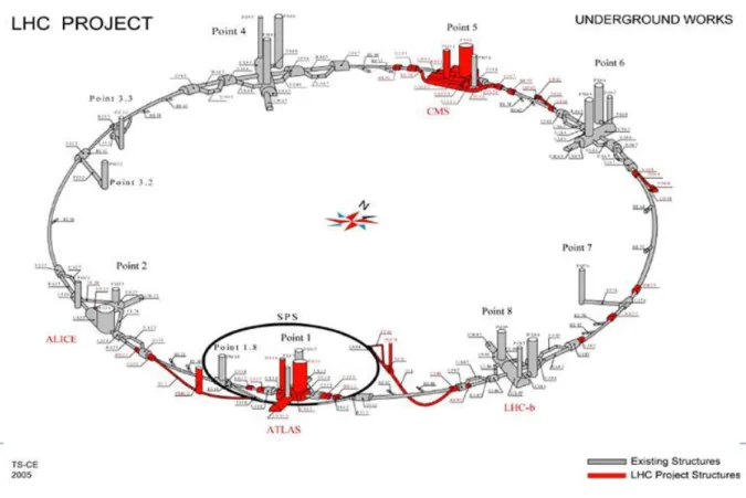
The large hadron collider 31

2.1.1 Structure 31

2.1.2 Acceleration 32

2.1.3 Luminosity 33

2.1.4 Beam Crossing and Pile-Up 34

2.2

The ATLAS Detector 35

2.2.1 Magnetic System 36

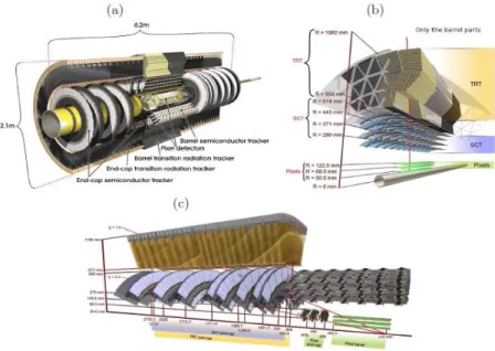
2.2.2 Inner detector 37

2.2.2.1 The Pixel Detector 37

2.2.2.2 The Semi-Conductor Tracker (SCT) 39

2.2.2.3 The Transition Radiation Tracker (TRT) 39

2.2.3 Calorimeters 39

2.2.3.1 Liquid Argon Electromagnetic Calorimeter (LAr) 40

2.2.3.2 Tile Hadronic Calorimeter 42

2.2.4 Moon spectrometer 43

2.3

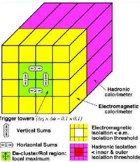
Event Trigger and Reconstruction 46

2.3.1 Event Triggering 46

2.3.2 Electron-Photon reconstruction and identification 48 2.3.3 Muon reconstruction and identification 51 2.3.4 Jet reconstruction and b-jet identification 51

2.3.5 Data Management and Efficiency 52

2.3.6 Data Management and Distribution 51

2.3.7 Data Efficiency 54

2.4

References 55

3

The Higgs to ZZ*

→

4L studies

57

3.1

Introduction 57

3.2

The H→ZZ(*)→4l channel 57

3.3

Data & Monte Carlo Samples 59

3.3.2 Monte Carlo Production 59

3.4

Event Selection 60

3.4.1 Trigger Application 60

3.4.2 Lepton Selection 60

3.4.3 Quadruplet Selection 61

3.5

Reducible Background estimation 63

3.5.1 Z+μμ background estimation 64

3.5.2 Z+ee background estimation 67

3.5.2.1 The 3l+X method 68

3.5.2.2 Transfer factor method using the Z+X±X± control region with 70 inverted cuts

3.5.2.3 Reco-truth unfolding method – relaxed cuts approach 73

3.5.3 Final Results on the background 78

3.6

Systematic Uncertainties 78

3.7

Final Results 80

3.8

Conclusions 84

3.9

References 86

4

Beyond Run 1: Phase II HL - LHC upgrades

89

4.1

ARTLAS Run 2 Upgrades 89

4.1.1 ATLAS Run 2 Upgrades 89

4.1.2 Physics motivation beyond Phase I 90

4.2

HL-LHC Upgrade Scenarios 91

4.3

References 95

5

Studies on the bbH(→γγ) channel at HL - LHC with 3000fb

-1

₉₇

5.1

Introduction 97

5.2

Physics Case 97

5.3

The bƃH(→γγ) mode 98

5.4

MC Samples 99

5.5

Object preselection and treatment 100

5.6

Analysis requirements 102

5.7

Event treatment and multiple combinations 105

5.8

TMVA Analysis 107

5.8.1 Results for a μ = 200 value 107

5.8.2 Results for a μ = 140 value 116

5.9

Cut Based analysis 119

5.10

Conclusions 121

5.11

References 123

6

Silicon detectors and simulations

125

6.1

Introduction 125

6.2

HL-LHC Requirements 125

6.3

Introduction to Silicon detector Fundamentals 126

6.3.1 Operating principles 128

6.3.2 Technologies and radiation damage 132

6.3.3 Charge collection and signal extraction 134

6.4

Introduction to Fundamentals of Pixel Sensor Simulation 136

6.4.1 Frameworks and available algorithms 136

6.4.2 Meshing strategy 137

6.4.3 Dopant Implantation models 138

6.5

Sensor Design and Active edge technology 141

6.5.1 The Active Edge technology 142

6.5.2 Design variations for the Multi-Project Run 143

6.6

Dopant Profile Characterization 144

6.6.1 Motivation 144

6.6.2 Secondary Ion Mass Spectroscopy as Tool for Simulation Validation 145

6.6.2.1 Measuring principals 145

6.6.2.2 Concentration Quantification 147

6.6.2.3 Depth Quantification 149

6.6.3 Test Production Characterization 152

6.6.3.1 n-in-n Test Wafer Samples 152

6.6.3.1.1 Sample Production Process 152

6.6.3.1.2 Process Simulation 154

6.6.3.1.3 Simulation – SIMS Comparison in Purely Silicon Samples 154

6.6.3.1.4 Oxide Layer Evaluation 159

6.6.3.1.5 High Resistivity Samples 159

6.6.3.1.6 Conclusions 161

6.6.3.2 n – in – p Test Wafer Samples 161

6.6.3.2.1 Wafer Fabrication 161

6.6.3.2.2 Sample Process Simulation 162 6.6.3.2.3 Simulation – SIMS Doping Profiles Comparison 163

6.6.3.2.4 Oxide Layer Evaluation 167

6.6.3.2.5 High Resistivity Samples 167

6.6.3.2.6 Conclusions 169

6.6.3.3 p-Spray Test Wafer Samples 169

6.6.3.3.1 Sample Production Processing 169

6.6.3.3.2 Process Simulation 169

6.6.3.3.3 SIMS- Simulation Doping Profile Studies 170

6.6.3.3.4 Conclusions 170

6.6.4 Low Gain Avalanche Diode Production Characterization 171

6.6.4.1 LGAD Principles 171

6.6.4.2 Test Structure Design 172

6.6.4.3 Sample preparation and measurements 173

6.6.4.4 Results for LGAD Run 7859 173

6.6.4.5 The Gallium Multiplication Region Test Run 177

6.7

Sensor Electrical Characterization 179

6.8

Under Bump Metallization (UBM) Influence on the sensor behavior 182

6.8.1 Introduction 182

6.8.2 The Discontinuity effect 183

6.8.3 Measurements and Results 184

6.8.4 Conclusions 185

6.9

Irradiated Doping Profiles 186

6.9.1 Introduction 186

6.9.2 n-in-n Irradiated Doping Profiles 187

6.9.3 p-Spray Irradiated Doping Profiles 188

6.9.4 Conclusions 191

6.10

Development of a Data Acquisition System for Pixel Detectors 191

6.10.1 Introduction 191

6.10.2 System Base Board – SPEC 191

6.10.3 The Multi-Level Interconnection Board (MLIB) 192

6.10.4 Conclusions 193

6.11

Conclusions on Pixel Development 193

6.12

References 193

8

Annexes

203

8.1

bbH Analysis Variables Discriminating Power and Distributions 203

8.2

The H(→bb)H(→γγ) mode 205

8.3

Doping Profile Simulation Reference Library 208

8.3.1 CiS n-in-n Test Wafers Simulation Parameters 208 8.3.2 VTT n-in-p Test Wafers Simulation Parameters 214

1 The Standard Model and the electroweak symmetry breaking

mechanism

1.1

The Standard model

The Standard Model (SM) of particle physics was developed over the second half of the 20th century and took its present form during the 70s. It effectively describes most of the interactions between elementary particles and since several decades, numerous experiments have tested and cer-tified its validity by verifying the predictions with an accuracy reaching 0.1 % in some cases [1].

The SM is a quantum field theory, based on gauge symmetry and expressed as a combination of SU(3)C × SU(2)L × U(1)Y groups [2]. The final product contains the symmetry group of strong in-teractions, SU(3)C, as well as the one corresponding to electroweak interactions, SU2L × U(1)Y. The group corresponding to electromagnetism, U(1)em, is included as a subgroup of the SU(2)L × U(1)Y product, since electromagnetic and weak forces are unified thanks to the works of Glashow [3], Salam [5] and Weinberg [4].

Elementary particles are divided into two main categories according to their statistical proper-ties, fermions and bosons. Fermions, (Figure 1.1 left) obeying Fermi - Dirac statistics are further distinguished into three families, whose members have similar properties but different masses. They are also classified into two categories, leptons and quarks. While leptons can exist in a free-state and exhibit full electrical load, quarks bare a fraction of electric charge in multiples of 1/3. They are subject to the strong interaction and are confined within states related to integer electric charge and to zero color. An antiparticle is associated with each fermion, with the same mass and statistic rules but opposite quantum numbers. Bosons (Figure 1.1 right) are integer spin particles obeying the Bose-Einstein statistics, allowing them to coexist in the same quantum state. Two types of bosons can be distinguished, with the first being spin s = 1vector fields, convening elementary interactions. The second type of bosons, with spin s = 0, has a single member so far, the so-called Higgs boson, that is a scalar field responsible for the electroweak symmetry breaking.

Figure 1.1: Standard Model particles and their properties. The fermions (left table) are the elementary con-stitutes of matter, while bosons (right table) act as mediators for all interactions.

The standard model gauge sector is composed of:

 Eight gluons, corresponding to the SU(3)C gauge bosons, responsible for the strong interac-tion that binds quarks together. Because of the color confinement, gluons and quarks cannot exist as free particles. Gluons have zero mass and unitary spin.

 The photon and the Z, W±,0

correspond to the gauge bosons of the electroweak interaction. The weak interaction is responsible for fission and beta decay. Its intensity is significantly

weaker than that of other elementary forces, while the short distance action indicates that the mediator bosons W±,0 _{and Z}0 _{are massive. The electromagnetic interaction, mediated by} the photon, is responsible for magnetic and electric phenomena. The range of the electro-magnetic force is infinite in the measure where the photon has a zero mass.

 Higgs boson: An additional - new type - boson, discovered in the summer of 2012, the Higgs boson is vital in understanding the spontaneous electroweak symmetry breaking. It has been at the epicenter of intense theoretical and experimental research for more than 50 years.

1.2

Gauge invariance in QED

To introduce gauge symmetries, the example of the quantum electrodynamics is often used. A spin ½ particle with mass m is described by the Dirac equation in its covariant form:

(𝐢𝛄𝝁_𝛛

𝛍− 𝐦)𝚿 = 𝟎 (1-1)

The corresponding Lagrangian can then be expressed in the following form: 𝐿𝑒= 𝛹̅(iγμ∂μ− m) (1-2)

which would consequently remain invariant under a phase transformation: 𝜳 → 𝒆𝒊𝜶_{𝜳 ⇔ (1-3)}

𝑳𝒆= 𝜳̅ (𝐢𝛄𝛍𝛛𝛍− 𝐦)𝜳 → 𝑳𝒆′ = 𝒆−𝒊𝜶𝜳̅ (𝐢𝛄𝛍𝛛𝛍− 𝐦)𝒆𝒊𝜶𝜳 ⇒ (1-4) 𝑳𝒆′ = 𝒆−𝒊𝜶𝒆𝒊𝜶𝜳̅ (𝐢𝛄𝛍𝛛𝛍− 𝐦)𝜳 ⇒ (1-5)

𝑳𝒆′ = 𝑳𝒆 (1-6)

On the contrary, if this phase transform is space dependent, then the Lagrangian invariance is lost:

𝜳 → 𝐞𝐢𝛂(𝐱)_{𝜳 ⇔ (1-7)}

𝑳𝒆′ = 𝒆−𝒊𝜶(𝐱)𝜳̅ (𝐢𝛄𝛍𝛛𝛍− 𝐦)𝒆𝒊𝜶(𝐱)𝜳 ⇒ (1-8) 𝑳𝒆′′= 𝑳𝒆 + 𝐞−𝐢𝛂(𝐱)𝜳̅ (𝐢𝛄𝛍(𝛛𝛍𝒆𝒊𝜶(𝐱)))𝒆𝒊𝜶(𝐱)𝜳 (1-9)

In order to preserve invariance, a covariant derivative introducing a gauge field Aμ is used, with respect to the following definition:

𝑫𝝁= 𝛛𝛍− 𝐢𝐞𝑨𝝁 (1-10)

where e represents the electron charge and is related to the coupling constant α of electromagnetic interaction by α = e2_{/4π ~ 1/137.}

The purpose of this new definition is to absorb the second term of the Lagrangian in the equation 1-9. Under a space dependent phase transformation, individual elements can be expressed in the following form: 𝜳 → 𝒆𝒊𝜶(𝒙)𝜳 (1-11) 𝑫𝝁→ 𝒆𝒊𝜶(𝒙)𝑫𝝁 (1-12) 𝑨𝝁→ 𝑨𝝁+ 𝟏 𝒆𝛛𝛍𝒂(𝒙) (1-13)

Gauge invariance of the free electron Lagrangian is therefore impossible unless we accept the existence of a gauge field Aμ. This would have to be a zero mass field, since a mass term in the form of mγ·2·Aμ·Aμ would render the Lagrangian non-invariant. By introducing the corresponding field coupling terms, in the form of Ψ(x)·AμΨ(x), one can observe that an interaction is mediated between free electrons. In reality, this field corresponds to the photon, mediator of electromagnetic interac-tions, with zero mass, while its coupling constant is identified as the elementary electromagnetic charge. The conclusive step left would be to describe the dynamics of this gauge field by introducing an additional term in the Lagrangian. We can define the electromagnetic tensor as:

F



     

 _  _ (1-14)

Finally, by expanding all terms, while using the definition of the tensor above, the Lagrangian can be expressed as:





1

4

e

L  i



 _ m   e



A_  FF_ (1-15)

1.3

Electroweak gauge invariance

In order to fully describe the electroweak interaction, three gauge fields are introduced. Two charged currents are needed (W±_{), as well as a neutral one (W}0_{) to achieve unification with} electro-magnetic interaction. This constraint imposes a representation by the SUL(2) group, being the mini-mum unitary group with the normal three-dimensional representation. The quantum number associated with this group is the weak isospin I. For the electromagnetic part, a unique gauge field is sufficient, so the choice of U(1)Y group is natural. The associated quantum number is the hyper-charge Y, a generalization of the electromagnetic hyper-charge.

In the context of the electroweak interaction SU(2)U(1) group, lepton representations corre-spond to SU(2) doublets:

, , e v v v e  





                     (1-16)

One could further separate these doublets of their right and left helicity by writing the corre-sponding spinors:



5





5



1 1 1 , R= 1 2 2 e e e e L R L e e e e         _{ }     _{ }   _{   }  _{   }         (1-17)

The electroweak interaction doesn’t preserve parity symmetry [6] resulting to the absence of right handed particles:













1 2 3 1 5 2 5 2 5 1 1 , 2 1 1 , 2 1 1 , 2 e e R L R L R L L e e e e L e L e                                _{   }            _{  } _            _{   }      (1-18)

1 1 2 2 3 3 1 2 3 , et d , c et s , t et b R R R R L R R R R L R R R R L u Q u u d d c Q c s s t Q t b b   _{ }       _{ }       _{ }     (1-19)

In order to unify the weak interaction isospin with the electromagnetic charge, a new quantity, the hypercharge, has to be introduced:

3

2 2

Y  Q I (1-20)

where Q is the charge and I3 the third component of the isotopic spin [7]. Using this definition, is possible to calculate hypercharge eigenvalues:

1 4 2 1 , 2 , , , Y 3 3 3 i Ri i Ri Ri L e Q u d Y   Y   Y  Y    (1-21)

The corresponding gauge fields on the mediator bosons would be the Bμ for Y generators of U(1)Y group as well as the three Wμ1,2,3 fields of the T1,2,3 generators corresponding to the SU(2) group. These generators are defined in the following way:

𝑻𝒊 =𝟏_𝟐𝝈𝒊 with σi the Pauli matrices (1-22) 𝑾𝝁𝝂𝒊 = 𝝏𝝁𝑾𝝂𝒊 − 𝝏𝝂𝑾𝝁𝒊 + 𝒈′𝒈𝝁𝝂𝑾𝝂

𝒋

𝑾𝝁𝒌𝑩𝝁𝝂 = 𝝏𝝁𝜝𝝂𝒊 − 𝝏𝝂𝜝𝝁𝒊 (1-23) where gμν denotes the anti-symmetric tensor.

In a similar manner as in the quantum electrodynamics case, in order to respect gauge invariance it is necessary to introduce a new covariant derivative in the Lagrangian that describes the electro-weak interaction. One can use:

"

'

2

i i

Y

D

_

  



_

_

ig TW

_



ig

B

_



_





(1-24)

with g΄ et g΄΄ the two coupling coefficients corresponding to the fields Bμ et de Wμ1,2,3 respectively. By continuing this approach, the electroweak Lagrangian can be written in the form of:

a a EW a a

1

1

L

= - W W

-4

4

i i i i i i i i R R i i R R R R

B B

L iD

L

e iD

e

Q iD

Q

u iD

u

d iD

d

             





















(1-25)

In this formula, the neutral bosons Wμ3 and Bμ correspond to linear combinations of the photon and the weak Z boson [8], while charged bosons W2_{, W}3 _{are equivalent to W}± _{bosons [9]. The} ab-sence of any mass term for all fields and in particular for the Wμ3 and Bμ components known to be massive because of their short action, has been a puzzling issue of the theory for years.

1.4

The BEH mechanism and electroweak symmetry breaking

The work of P. Higgs [10], F. Englert and R. Brout [11], G.S. Guralnik et al. [12] resulted in a model that explains the appearance of the weak force mediators masses through the spontaneous breaking of electroweak symmetry, while keeping photons and gluons massless.

1.4.1 The BEH mechanism

Particles can acquire mass through their interaction with the Higgs field. The mechanism attrib-utes mass to the bosons by absorption of Nambu - Goldstone bosons, occurring from the spontaneous symmetry breaking. In its simplest expression, an additional field, the Higgs, is added to the gauge theory. The spontaneous breaking of the underlying local symmetry triggers the conversion of the field components to Goldstone bosons, interacting with the other fields of the theory in order to produce the mass terms of the gauge bosons. This mechanism leaves behind a scalar elementary particle (spin 0), known as the Higgs boson, while respecting the need of a massless photon.

To generate masses for the W and Z bosons while maintaining the U(1)em unchanged, one has to break the SU(2)L × U(1)Y symmetry. To do so, a neutral component of a scalar complex field doublet is introduced. † 0

, Υ



1









 

_

_







(1-26)

This new field can be fully described by the following Lagrangian:

 

†

 

_{2 †}

 

_† 2

H

L



D

_



D



      





(1-27)

where Dμ the covariant derivative defined at the electroweak interaction and μ, λ are unknown con-stants. The kinetic term is already included in the expression [(DμΦ*)(DμΦ)] along with a potential term [V=μ2 _Φ*_Φ+λ(Φ*_Φ)2_{], the most generic possible while respecting SU(2) invariance. By fixing} one of the parameters assuming λ > 0, we can examine the behavior for different values of μ2_{. If the} latest is positive, then the potential nominal value would be zero. On the contrary, if μ2 _{is considered} negative, the potential will develop a non-zero vacuum expectation value (Figure 1.2).

The kinetic term of the Lagrangian also contains the mass factor of the boson associated with the Higgs field. This originates from the second neutral component of the field. Both components, the charged one and one of the neutrals, are Goldstone bosons, acting as the third component of longitudinal polarization of massive W± _{and Z bosons. The remaining neutral component is} associ-ated with the massive Higgs boson. Since the Higgs field is a scalar, the corresponding gauge boson has spin zero, no electric charge or color, while its wave function is symmetric.

Figure 1.2: Form of the Higgs potential in the complex plan for positive (a) or negative μ2 _{(b) The small} sphere indicates a possible choice for the direction of the potential vector.

The vacuum expectation value can be computed from the potential by applying the operator to the wave function:

^ 2 0 0 1 0 0 2           _{  }     (1-28)

The 1 2factor is imposed by the normalization requirement. The minimum expected value is calculated as the absolute value of _{ }2 , estimated from the Fermi constant to be ~ 246 GeV. This form of potential is more commonly known as “The Mexican Hat Potential”, since its initial value, or vacuum value, is non-zero. There are infinite possibilities of passing to a stable minimum, which causes the symmetry breaking by leaving the initial value. Keeping in mind the demand to maintain U(1)em while breaking the SU(2)L × U(1)Y symmetry, from the infinite amount of algebraic solutions implied by equation 1-28, an appropriate suggestion for the wave fiction representation is the fol-lowing:

𝛗 = (𝟎𝐯 √𝟐

) (1-29)

Although an analytic solution for the Lagrangian (equation 1-27) would not be possible in its general form, one can approach the problem by an expansion at the minimum potential value [13]. Since the appearance of the Goldstone bosons is intrinsic on the theoretical side, it is convenient to use a parameterization that would eliminate the corresponding terms:

𝝋 → 𝝋′ =𝒆 𝒊𝝈𝒂(𝒙) 𝒗 √𝟐 ( 𝟎 𝒗 + 𝒉(𝒙)) (1-30)

Expanding the Lagrangian at the minimum potential value using equation 1-30 we can derive at the fourth order term approximation:

𝐋 =𝟏 𝟐𝛛𝛍𝐡𝛛 𝛍_{𝐡 −}𝟏 𝟐𝛌𝐯 𝟐_𝐡𝟐_{− 𝛌𝐯𝐡}𝟑₋𝛌 𝟒𝐡 𝟒₊ +𝟏_𝟐[𝐠′𝟐_𝟒𝐯𝟑𝐁𝛍𝐁𝛍− 𝐠𝐠′_𝐯𝟐 𝟐 𝐖𝛍 𝟑_𝚩𝛍₊𝐠𝟐𝐯𝟐 𝟒 𝐖𝛍𝐖 𝛍_] +𝟏 𝐕[ 𝐠′𝟐𝐯𝟐 𝟒 𝐁𝛍𝐁 𝛍_{𝐡 −}𝐠𝐠′𝐯𝟐 𝟐 𝐖𝛍 𝟑_𝚩𝛍_{𝐡 +}𝐠𝟐𝐯𝟐 𝟒 𝐖𝛍𝐖 𝛍_𝐡] + 𝟏 𝐯𝟐[ 𝐠′𝟐𝐯𝟐 𝟒 𝐁𝛍𝐁 𝛍_𝐡𝟐₋𝐠𝐠′𝐯𝟐 𝟐 𝐖𝛍 𝟑_𝚩𝛍_𝐡𝟐₊𝐠𝟐𝐯𝟐 𝟒 𝐖𝛍𝐖 𝛍_𝐡𝟐_{] + ⋯} (1-31)

 The first term of equation 1-31 represents the Higgs field dynamics as well as the par-ticles mass as a function of the potential vacuum expectation value, mH2=2λv2.  Subsequent terms on the second line generate W±_{, Z bosons masses. The B}

μ and Wμ3 are mixed together in the first two terms, with one of them generating the QED photon field Aμ of zero mass. Z boson mass can appear by deagonalizing the mixing matrix with the help of the weak interaction angle θw according to the following definition:

𝟏 𝟒( 𝒈𝟐_𝒗𝟐 _−𝒈𝒈′𝒗𝟐 −𝒈′_𝒈𝒗𝟐 _𝒈′𝟐_𝒗𝟐 ) = 𝑴 −𝟏_(𝒎𝒛𝟐 𝟎 𝟎 𝟎) 𝑴 , 𝑴 = ( 𝐜𝐨𝐬 (𝜽𝒘) −𝐬𝐢𝐧 (𝜽𝒘) 𝐬𝐢𝐧 (𝜽𝒘) 𝐜𝐨𝐬 (𝜽𝒘)) (1-32) It can be deducted that mz2= (g2+g’2)v2/4

 The W± _{is included in the third term of the second line within the multiplication factor:} 𝒈𝟐𝒗𝟐 𝟒 𝑾𝝁𝑾 𝝁_→𝟏 𝟐𝒗𝒈 | 𝟏 √𝟐(𝑾 `𝟏<sub>∓ 𝑾</sub>`𝟐_{)| → 𝒎} 𝒘= 𝟏 𝟐𝒗𝒈 (1-33)

 The two last lines of the Lagrangian describe the interaction of the Higgs boson with the W, Z and γ boson fields.

Although for the boson case the mass generation is straight-forward appearing in the Lagran-gian, fermion masses are not explained. Adding a mass term to the theory in the form of 𝑚(𝐿𝐿̅ + 𝑅𝑅̅) would not be possible since this would violate the SU(2)L gauge invariance. Instead, one can introduce indirect interactions with the Higgs field via Yukawa couplings in the initial Lagrangian which for the electron case would take the form:

𝑳𝑯= −𝝀𝒆(𝑳̅𝒍𝝋𝑹𝒍+ 𝑹̅̅̅𝝋𝒍 †𝑳𝒍) (1-34) By applying the spontaneous symmetry breaking 𝜑 → 𝜑′ = 𝟏

√2( 0

𝑣 + ℎ(𝑥)) in the same manner as for the bosons equation 1-34 becomes:

𝑳𝑯= − 𝝀_𝒆𝒗

√𝟐𝝍̅𝒍𝝍𝒍− 𝝀_𝒆

√𝟐𝝍̅𝒍𝝍𝒍𝒉 (1-35)

In this form, the first term corresponds to the electron mass, while the second represents the Higgs coupling to the electron and hence proportional to the electro mass. By repeating the same process for each lepton all the masses can be generated, whereas a constant g is introduced in each case.

In the quark case, the process remains identical with the exception of the up-type particles where a rotation of the Higgs field has to be considered in the form of:

𝝋 → 𝝋′ = 𝟏 √𝟐(

𝒗 + 𝒉(𝒙)

𝟎 ) (1-36)

In a nutshell, the Higgs mechanism introduces the mass for all the gauge bosons and fermions as described in Table 1-1. The unavoidable side-effect is the introduction of a new massive field associated with a corresponding scalar boson, the Higgs boson. The corresponding couplings are proportional to the generated masses and for all intents and purposes are described as λf for the fermions, λb for the bosons and λ for the Higgs self-coupling.

Boson masses _{𝑚𝑏 =}𝜆𝑏𝑣 2 Fermion masses 𝑚𝑓 = 𝜆𝑓𝑣 √2 Higgs mass _{𝑚𝐻 = √2𝜆𝑣}2

Table 1-1: Generated mass of the Standard Model particles and their corresponding formulas.

1.4.2 The Higgs boson mass

The Higgs boson mass is a free parameter of the model and can be constrained indirectly by several higher order effects present in loops, resulting in tiny corrections in various precision meas-urements of the electroweak parameters. Thus, the fit of the most precise results obtained essentially from LEP experiment have been used for a long time to extract a most probable Higgs mass field’s value [1].

The mass of the Higgs boson can be calculated from the following formula:

2

2

H

Since μ is related to λ with respect to the vacuum expectation value of the potential, 𝑣 = √𝜇2_{⁄ 𝜆} and λ is not fixed, mH remains unknown. Before the discovery, constraints have been imposed by considering the unitarity of the standard model, triviality and the vacuum stability.

Perturbative unitarity: While considering the case of W bosons elastic scattering, the corre-sponding cross-section increases with respect to scattering energy, violating the principle of unitarity around ~ 1 TeV. In order to restore balance to the theory, the Higgs mechanism introduces and additional interaction diagram through its coupling with the W boson. This interaction path restores equilibrium for the increasing contributions with respect to the energy value for certain values of the Higgs mass. The corresponding upper limit is:

𝒎𝑯= (𝟖𝝅√𝟐_𝟑𝑮

𝑭) ≈ 𝟕𝟎𝟎 𝑮𝒆𝑽/ 𝒄

𝟐 _(1-38)

Triviality: Consideration of higher order relative corrections in Higgs self-coupling constant λΗ, introduces an energy dependence of this very constant (“running coupling constant”). This al-lows the extraction of a limit for the Higgs mass of around ~ 160 GeV [14], for a validity up to the 1016 _{GeV scale.}

Vacuum stability: The argument of vacuum stability is based on the fact that the Higgs potential has to always be limited with respect to its minimal value. This means that the coupling constant λ(Q) has to remain positive, introducing a lower limit on the Higgs mass. In fact, if λ becomes extremely small, top quark and weak boson loops start to appear due to their strong coupling with the Higgs field. As a result, λ could become negative and the vacuum would become unstable since no minimum value would exist [15]. The constraint of a positive coupling content λ(Q2_{) implies that} mH > 70 GeV/c2 for a validity of the Standard Model up to the TeV scale. Figure 1.3 presents im-posed limits on the Higgs mass with respect to the validity scale of the Standard Model.

Figure 1.3: Lower and higher limits of the Higgs mass with respect to the standard models validity scale (μ2 _{< 0).}

1.5

Higgs production modes at hadronic colliders

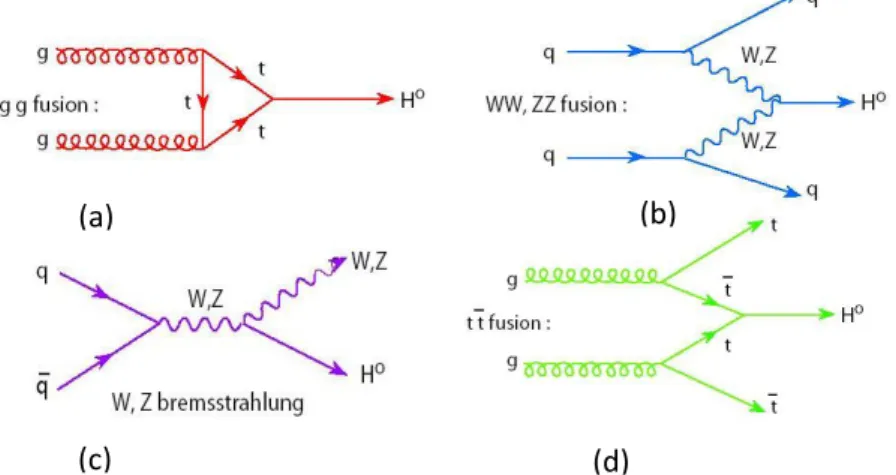
Four main processes exist for the production of the Higgs boson in hadronic colliders:  Gluon fusion (Figure 1.5 a)

 Vector boson fusion (VBF) (Figure 1.5 b)

 Associated production with W or Z bosons, also known as Higgsstrahlung (Figure 1.5 c)  Associated production with a quark pair, mainly the 𝑡𝑡̅ (Figure 1.5 d)

At LHC energies (Figure 1.4), the dominant Higgs production process is gluon fusion. Since the Higgs boson is not coupled with gluons, its production is carried out indirectly through quark loops and notably the top. This production mode is at least one order-of-magnitude larger than all other production processes because of the gluon component abundance in the colliding protons at the LHC energy range.

Figure 1.4 : Cross section of the various Higgs production modes as a function of the collision energy, for 7 TeV < √𝒔 < 14 TeV [16].

The second most important mode is the vector boson fusion (VBF). This process demonstrates a particular topology. The quarks interact through a W or Z boson, indicating that this is an electro-weak process and does not imply a color exchange between the initial and final quark states. The two final quarks generate forward jets in opposite hemispheres inside the detector, making a clear topology which allows for a very good signal-to-background separation.

A Higgs boson can also be produced in association with a W/Z boson. One of the initial quarks of the colliding protons can annihilate with an antiquark, producing in the final state a real Z or W in conjunction with a Higgs boson.

The last production mode comes from a heavy quark pair (top or bottom). Quite often, in proton collisions, a gluon or quark pair can annihilate generating a pair of heavy quarks. Those can fuse generating a Higgs boson in the processes. This phenomenon is quite rare, estimated at least 100 times less significant with respect to the gluon-gluon fusion mode.

Figure 1.5: Feynman diagrams for the main Higgs production modes. From top left to bottom right: gluon fusion process (a), vector boson fusion (b), quark-quark scattering (c) and quark gluon annihilation (d) also

referred as Higgsstrahlung. (d)

(a) (b)

The VBF and W/Z or top associated production modes are of different nature with respect to the gluon-gluon fusion process, in the sense that the final Higgs boson is produced in association with additional objects at the final state. This allows for a better signal to background separation although the sensitivity is generally reduced in low luminosity. All production modes are being con-sidered in the Higgs boson studies. In LHC conditions, due to the proton-proton composition of the beam, qq scattering is favored and VBF is the second most important production mode after the dominant gluon-gluon fusion mode.

Figure 1.6: The LHC SM Higgs production cross-section for the five most prominent modes at a √𝒔 = 𝟕 𝑻𝒆𝑽 (left) and √𝒔 = 𝟏𝟒 𝑻𝒆𝑽 (right) center of mass energy.

Computation of the Higgs boson production cross-section in the various modes requires to take into account higher order corrections. Recently, Anastasiou et al. [17] achieved the long-waited NNNLO computation of the main production mode gg→H. This major accomplishment permits the understanding of gluon-gluon fusion cross-section within a ~ 3 % uncertainty. In this computation, an additional source of uncertainty comes from the Parton Density Functions (PDF) used, presently known within 2 – 3 % precision [18]. These two major breakthroughs have been achieved after the end of Run 1 of LHC.

1.6

Higgs decay channels

Higgs decay modes can be distinguished into three main categories:

 Prompt decays to a particle-antiparticle pair (quarks: 𝑐𝑐̅, 𝑠𝑠̅, 𝑡𝑡̅, 𝑏𝑏̅ and leptons: 𝜇𝜇̅, 𝜏𝜏̅)  Decays though virtual loops (top, W)

 Decays to vector bosons WW* and ZZ*

Feynman diagrams for the different Higgs decay modes are illustrated in the following figure (Figure 1.7):

As for the mass of the Higgs, the coupling constants for bosons and fermions are not fixed by the theory. The branching fractions of the various modes are shown relative to the mass of the boson (Figure 1.8). Higgs couples preferentially with the most massive particles, therefore, the most im-portant branching ratios would be to the heaviest particles allowed by the Higgs mass value.

In the fermion case, the decay width can be expressed using the color factor Nc (Nc= 1 for leptons and Nc = 3 for quarks), the original fermion and Higgs particle masses as well as the mini-mum potential value. The color factor is introduced when final decay products carry color charge in order to ensure a colorless fermion - antifermion final state, since the Higgs field is colorless. As a result, decay width is formulated in the following way:

𝜞(𝑯 → 𝒇𝒇̅) =𝒎𝑯 𝟖𝝅 ( 𝒎𝒇 𝒗) 𝟐_𝑵 𝒄(𝟏 − 𝟒𝒎_𝒇𝟐 𝒎_𝑯𝟐) 𝟑 𝟐 ⁄ (1-39)

Except for the top case, where the approximation (mH >> mf) is no longer valid, one can ap-proximate the formulation by considering the fermion mass significantly smaller with respect to that of the Higgs. The last term of the width expression then becomes increasingly close to the unity and we can safely assume that the final resonance width or the fermion decay is proportional to the boson mass. Conversely, decays to top quarks would only come from a Higgs mass around twice that of the quark. For the fermion decays, one can notice that the widths are linear as a function of the Higgs mass.

Figure 1.8: Branching ratio for the different decay Figure 1.9 : Variation of the natural Higgs width modes foreseen in tree-level SM [14]. with respect to the particle mass. Considering bosonic decays, a slightly altered approach has to be considered for the massive electroweak (W± _{and Z) and massless photon and gluon cases. In the electroweak case, no color} compensation factor has to be included since there is no possible mediation of color charged objects but the indistinguishable nature of the outgoing W± _{field for a neutral Higgs case impose the} intro-duction of an additional factor of two at the WW decay width. Except for the additional mass change, calculations are identical, yielding widths described correspondingly by the representations:

𝜞(𝑯 → 𝒁𝒁) = 𝒎𝑯 𝟑𝟐𝝅( 𝒎𝑯 𝒗𝟐) 𝟐_{(𝟏 −}𝟒𝒎𝒁𝟐 𝒎_𝑯𝟐) 𝟏 𝟐 ⁄ [𝟏 − 𝟒 (𝒎𝒁𝟐 𝒎_𝑯𝟐) + 𝟏𝟐 ( 𝒎_𝒁𝟐 𝒎_𝑯𝟐) 𝟐 ] (1-40) 𝜞(𝑯 → 𝑾𝑾) =𝒎𝑯 𝟏𝟔𝝅( 𝒎𝑯 𝒗𝟐)𝟐(𝟏 − 𝟒𝒎_𝑾𝟐 𝒎_𝑯𝟐 ) 𝟏 𝟐 ⁄ [𝟏 − 𝟒 (𝒎𝑾𝟐 𝒎_𝑯𝟐) + 𝟏𝟐 ( 𝒎_𝑾𝟐 𝒎_𝑯𝟐) 𝟐 ] (1-41)

As previously stated, in the mH > mw,z case, the second term of the width formulation increas-ingly tends towards unity, while 1/mH dependence can be derived for the last term when approxi-mated by a converging sequence. Overall, the width dependence would be proportional to ̴ mH3, rendering the increase in the resonance width faster than in the fermions case.

From the previous width formulas (equations 1-39, 1-40 and 1-41) it can be concluded that Higgs decays preferably to the most massive particles allowed by its rest-mass value. This implies zero interaction with massless particles like gluons and photons at tree level. The di-photon final state is rare because of solely loop coupling with the photon. This decay is realized through top quark and W boson loops. Despite the small branching ratio, this mode remains very important with a very clear signal into two photons in the end state. It allows direct measurement of the mass boson.

In the width calculation, one can use the same approximations for all massless bosons, gluons and photons, with the caveat of including the color-factor in the photon case as well as the electric charge of the intermediate fermion (Qf), while for gluons the δΑΒ needs to be introduced to ensure that the intermediate fermionic pair is colorless. In more detail the corresponding width for the gluon decays is: 𝜞(𝑯 → 𝒈𝒈) = 𝒂𝒂𝒔𝟐𝒎𝑯𝟑 𝟐𝝅𝟐_𝒎 𝒘 𝟐_𝒔𝒊𝒏𝟐_𝜽 𝒘|∑ 𝑰( 𝒎_𝑯𝟐 𝒎_𝒒𝟐) 𝟐 𝒒 | (1-42)

Where I is the form factor integral [19]. Concerning the photon case calculations, an additional complexity is imposed by the number of available interaction diagrams and the different possible topologies (26 in total for the W –loop case). Using the same approach as before one can approxi-mate: 𝚪(𝐇 → 𝛄𝛄) ≈ 𝐚𝟑𝐦𝐇𝟑 𝟐𝟓𝟔𝛑𝟐_𝐦 𝐰 𝟐_𝐬𝐢𝐧𝟐_𝛉 𝐰|𝟕 − 𝟏𝟔 𝟗 + ⋯ | 𝟐 (1-43)

Terms within equation’s 1-42 last factor correspond to W, top, etc. loop contributions respec-tively, while the most predominant one is the W contribution of the initial term. Given the proximity of the W mass value to that of the Higgs (≈ 2/3 of mH) and its region in the mass scale, when appro-priate approximations are applied to equations 1-43 and 1-34, it is derived that the dependence of the Higgs resonance width is proportional to mH2 in both the gluon and photon case, thus making it uniform for all bosonic decay modes.

The relative importance of a decay mode is qualified within the standard model by its branching ratio (Figure 1.8):

ß𝒓

_𝒊

=

𝚪𝒊

𝚪𝒕𝒐𝒕 (1-44)

where Γi denotes the Higgs decay width to the ith channel. Figure 1.10 presents the dependence of the total Higgs width on its mass, varying from 4.2 MeV at 125 GeV to 100 GeV at 500 GeV. The 125 GeV mass of the discovered boson allows for a narrow total width, far below any achievable detector resolution, making experimental performances the most dominant effect in any combined Higgs mass or decay width measurement.

1.7

Current Status of Higgs measurements

1.7.1 Mass measurement

The final result on the mass of the new boson was published by the ATLAS collaboration in July 2014, considering all available Run 1 data. Using a total integrated luminosity of 25 fb-1_, im-proved analysis approaches and better control of systematics, the H→γγ and the H→ZZ*→4l chan-nels were combined to extract the most precise mass estimation. In the di-photon channel, 475.9 events are expected following the Standard Model prediction, while for the four lepton final state, this number is reduced to 26.5 events. By combining the corresponding measurements, the ATLAS measured mass value is estimated at:

mH= 125.36±0.37(stat)±0.18(syst) GeV (1-45)

where the total uncertainty is dominated by the statistical term [20]. Figure 1.11 presents the ratio of the profiled likelihood defined as:

𝜦(𝒎𝑯) =

𝑳(𝒎𝑯,𝝁̂𝜸𝜸(𝒎𝑯),𝝁̂𝟒𝒍(𝒎𝑯),𝜽̂ (𝒎𝑯))

𝑳(𝒎𝑯,𝝁̂𝜸𝜸,𝝁̂𝟒𝒍,𝜽̂) (1-46)

where mH represents the probed Higgs mass and μγγ – μ4l are the signal strengths for the di-photon and four lepton channels respectively, treated as nuisance parameters in the final fit [21]. The pro-filed likelihood variations in the two individual channels and the combination are propro-filed as a func-tion of the mH. The Higgs boson masses estimated with the di-photon and the four-lepton channels are compatible within 1.98 sigma (δmH=1.47±0.72 GeV).

Figure 1.11: Scans of the negative log likelihood with respect of the Higgs mass for ATLAS experiment in each channel and the total combination, in black. Dashed curves show the results accounted for statistical

A corresponding combination was also published by the CMS experiment evaluating all avail-able data on the di-photon and the four lepton channels. The two collaborations use diverse detector technologies and analogous analyses approaches. A similar combination campaign has been driven among the two collaborations to fully exploit the total LHC statistics [22]. Theoretical and model uncertainties, which are identical to both experiment, are considered to be completely correlated, while uncertainties connected to detector design, specifically the momentum scale and the resolution of objects, are unique to each experiment and are considered uncorrelated. Combining all available data, the mass of the Higgs boson at LHC is found to be:

mH = 125.09±0.24 GeV

= 125.09±0.21(stat)±0.11(system) GeV (1-47)

The impact of each uncertainty category can be assessed by fixing the corresponding nuisance parameters to their best fit values increased or decreased by 1 σ, while the rest are being profiled. In a breakdown it can be calculated:

mH = 125.09 ± 0.21 (stat.) ± 0.11 (scale) ± 0.02 (other) ± 0.01 (theory) GeV (1-48) Although both collaborations have improved the understanding of their detector and its perfor-mance since Run 1, it is clear that the scale uncertainties dominate the systematic term.

The mass evaluation of the individual channels (H→γγ and H→ZZ) have also been combined between the two experiments. Figure 1.12 presents the summary of the individual and combined channels. Small tensions are observed between the ATLAS and CMS H→γγ and H→ZZ* masses at the level of less than 1.5 sigma. The final mass value is again limited by statistics, while the most important systematic uncertainty is related to the energy and momentum precision in both experi-ments.

Figure 1.12: Consistency between different results of the ATLAS and CMS collaborations in the two com-bined channels for Run 1 data.

1.7.2 Couplings Estimation

Measurement or constraint of the Higgs production and decay modes has been performed by both ATLAS and CMS. Main production processes include gluon-gluon fusion, VBF component and associated production with mainly top quark. The studied decay channels concern bosonic final states (ZZ, WW, γγ) and fermionic ones (bb, ττ, μμ). In the following table significances and limits

for each treated mode are presented with corresponding uncertainties from both ATLAS and CMS collaborations (Table 1-2).

Channel Signal Strength (μ) Signal Significance (σ)

ATLAS CMS ATLAS CMS H→γγ 1.15−0.25+0.27 1.12−0.23+0.25 5.0 5.6 H→ΖΖ*→4l 1.51−0.34+0.39 1.05−0.27+0.32 6.6 7.0 H→WW 1.23−0.21+0.23 0.91−0.21+0.24 6.8 4.8 H→ττ 1.41−0.35+0.40 0.89−0.28+0.31 4.4 3.4 H→bb 0.62−0.36+0.37 0.81−0.42+0.45 1.7 2.0 H→μμ −0.7−3.6+3.6 0.8−3.5+3.5 ttH 1.9−0.7+0.8 2.9−0.9+1.0 2.7 3.6

Table 1-2: Measured significances and signal strength for all Higgs primary decay modes by both ATLAS

and CMS collaborations.

In the hypothesis that the Higgs boson width (predicted to be 4 MeV for the SM) is sufficiently small for the narrow width approximation to be valid, production and decay processes can be de-composed and factorized. Using this factorization, a specific process i→H→f, where i denotes the initial state and f the final product, can be described by the product of the production mode cross-section multiplied by the branching ration of the final state in the following manner (equation 1-49):

σi×BRf= σi× ( Γf / ΓH ) (1-49)

where σi is the cross-section of the production process, BRf the branching ratio of the final state, ΓH the total natural width of the Higgs and Γf the Higgs decay width in the probed final state.

Combination of the coupling results from the two collaborations has been performed to increase the testing sensitivity of the SM predictions. Because measurement of the yield of a Higgs decay channel is not enough to determine the cross-section and the branching ratio independently, various methods have been developed in LHC to probe the compatibility of the results with SM expectations. To bypass the lack of full information, one of the parameterizations applied in the combination uses normalized yields of i→H→f to the gg→H→ZZ rate. This choice is driven by the fact that the corresponding section presents the smallest overall uncertainty. Calculating ratios of cross-sections and branching ratios yields results independent from any theoretical uncertainties on abso-lute rates.

The observed number of H→ZZ*_{→4l events are expressed as the product of the gluon-gluon} fusion Higgs production cross-section multiplied by the ZZ* channel branching ratio (equation1-50):

𝜎𝑧𝑧= 𝜎𝑔𝑔𝐹𝐻 × 𝐵𝑅𝑍𝑍 ⇒ 𝜎𝑔𝑔𝐹𝐻 = 𝜎_𝑧𝑧

𝐵𝑅_𝑍𝑍 (1-50)

Using this definition, the cross-sections of all other processes can be expressed as yields with respect to the four lepton channel. For the di-photon case it would be (equation 1-51):

𝜎𝛾𝛾= 𝜎_𝑧𝑧

𝐵𝑅_𝑍𝑍× 𝐵𝑅𝛾𝛾 ⇒ 𝜎𝛾𝛾 = 𝐵𝑅_𝛾𝛾

𝐵𝑅_𝑍𝑍 × 𝜎𝑧𝑧 (1-51)

In that way, one can evaluate all cross-sections as yields with respect to the ZZ production channel.

Figure 1.13 presents the per-experiment and the combined values of the cross-sections and of the branching ratios for various production and decay modes. Each ratio is normalized to the SM prediction such as, assuming model validity, all ratios would be unitary. All available Run 1 data (at 7 and 8 TeV) are included in the fit with the global compatibility hypothesis to SM (ratios ≈ 1)

having a p-value of 10-6_{. In this figure, the most precise measurements are indeed in agreement with} the SM within less than 2 sigma [23]. The largest deviations are due to the ttH channel (2.3 sigma deviation) and to the ZH (excess observed only in CMS data [25]). The smallest ratio is observed in the Brbb/BrZZ case. For bb analyses, the proper associated production mode (ZH(→bb)) is studied, since it allows an increased rejection of the continuum b-quark QCD background through the use of the Z decay leptons. The cross-section in this case is expressed as (equation 1-52):

𝜎_𝑏𝑏𝑍𝐻 = 𝜎_𝑍𝐻𝐻 _{× 𝐵𝑅} 𝑏𝑏 ⇒ 𝜎𝑏𝑏𝑍𝐻 = 𝜎𝑍𝐻𝐻 × 𝜎_𝑧𝑧 𝐵𝑅_𝑍𝑍× 𝐵𝑅_𝑏𝑏 𝜎_𝑔𝑔𝐹𝐻 ⇒ 𝜎𝑏𝑏 𝑍𝐻 _{= 𝜎} 𝑍𝐻𝐻 × 𝐵𝑅_𝑏𝑏 𝐵𝑅_𝑍𝑍× 𝜎_𝑧𝑧 𝜎_𝑔𝑔𝐹𝐻 (1-52) The measured cross-section ratio σZH / σZZ is quite significant (close to 3) as shown in the same figure. As a result, the branching ratio of bb decay over the ZZ channel branching ratio is found to be reduced with respect to SM predictions, in order to keep the measured number of events to the observed rate. Search for the H→bb decay by both collaborations yields signals with low signifi-cances [24, 25], of 1.7 and 2.0 sigma for ATLAS and CMS respectively.

Figure 1.13: Best fit values for cross-sections, ratios of cross-sections and branching ratios from ATLAS and CMS experiments data. The ATLAS and CMS combined values are shown in black.

1.8

Conclusions

It is a triviality to emphasize the impressive harvest of results on the Higgs Boson research achieved by the LHC experiments using Run 1 data samples. This is however only the beginning of the Higgs era, since a lot of information concerning the properties of the new boson is still missing: not all not all production modes nor all decay channels have been identified. The jump in energy and in luminosity expected at Run 2 will allow to collect a gigantic amount of Higgs data, which will be utilized to enrich the available anthology of the boson properties.

During the next phases of the accelerator, the LHC collaboration will be able to examine to an unprecedented detail the nature of the Higgs mechanism and to probe the existence of new sectors of physics.