Aléa sismique et gravitaire en zone de montagne : application au Cachemire (Pakistan)

HAL Id: tel-00684242

https://tel.archives-ouvertes.fr/tel-00684242

Submitted on 31 Mar 2012

HAL is a multi-disciplinary open access archive for the deposit and dissemination of sci-entific research documents, whether they are pub-lished or not. The documents may come from teaching and research institutions in France or abroad, or from public or private research centers.

L’archive ouverte pluridisciplinaire HAL, est destinée au dépôt et à la diffusion de documents scientifiques de niveau recherche, publiés ou non, émanant des établissements d’enseignement et de recherche français ou étrangers, des laboratoires publics ou privés.

application au Cachemire (Pakistan)

Mohammad Tahir

To cite this version:

Mohammad Tahir. Aléa sismique et gravitaire en zone de montagne : application au Cachemire (Pakistan). Sciences de la Terre. Université de Grenoble, 2011. Français. �NNT : 2011GRENU052�. �tel-00684242�

&'(!%)*+&%+,-)./0%*$/!1+&%+2*%.'3,%

B@C;AA;9+!D"/*

DL?6<8C@4M+N<@N6<?568+;79+5?8+

?<5OO6<57O+A64C;758A

On the last decades, progresses on the understanding of clustering seismicity in time, size and space have been driven by two parallel approaches. From the one hand studies on the mechanics of faulting in an elastic medium argue for the static stress triggering to dominate in the near field, i.e within distance less than 10 fault length. From the other hand, mean field properties of the triggering are reproduced using cascading effects in point process models. In this study we try to reconcile these approaches by emphasizing the importance of faulting style on average properties of seismicity. Starting with the study

of the seismicity rate triggered by the Muzaffarabad, Kashmir, 2005 Mw = 7.6, Ms = 7.7

earthquake, which appears as above the average when analysing the aftershocks sequences in the India-Asia collision belt, we resolve the strike slip event productivity to be on average 4 times smaller than the thrust faulting productivity. Using global earthquake catalog, we further extend this result as all the parameters of the Omori law (p, K, α, N(t)) being dependent on faulting styles. Within the ETAS model strong K, N and low α values are driven by high branching ratio (n). As consequences of the relative high n − value of the thrust events, it also predicts a lower p − value for thrust event as compare to

strike slip and normal events as the pN > pSS > pT we observe. Within rate and state

friction framework it implies a change in stress heterogeneity patterns. We do not resolve

any robust changes in foreshocks rate, p!_{− value, whereas our analysis allow us to extend}

B˚aths law in time, space and focal mechanism. For reverse faults, both the magnitude

difference and the distance from the mainshock to the largest aftershock are somewhat less than for strike slip faults. The distribution of time intervals between mainshocks and their

occurs earlier than later in a given sequence of aftershocks. Moreover, this finding argues for going beyond the branching point model, with implications for short term forecasts. Also we resolve unambiguous dependency of p − value of Omori law to mainshock magnitude for the aftershock within 10 days after the mainshock occurrence, this dependency being lost when using complete cascade sequences. We find this time threshold also corresponds to a change in diffusion patterns, all these changes synchronize with the occurrence of the largest aftershock. Accordingly, our results converge toward the key role of the secondary aftershocks on the mechanics of size, time and space pattern of cascading processes.

Au cours des derni`eres d´ecennies, des progr´es ont ´et´e r´ealis´es sur la compr´ehension des r´epliques de s´eismes dans les domaines spatio-temporels. D’une part des ´etudes sur la m´ecanique dune faille dans un milieu ´elastique montrent que le d´eclenchement statique domine le d´eclenchement des r´epliques dans le champ proche, i.e., une distance de moins de 5-10 *L, (L, longueur de la faille sismique). D’autre part les propri´et´es du champ moyen du d´eclenchement sont reproduites `a l’aide de cascade dans des mod`eles de branchement. Au cours de cette th´ese, nous avons tent´e de concilier ces 2 approches en mettant en ´evidence l’importance du type de faille sur les propri´et´es moyennes de la sismicit´e d´eclench´ee, i.e. les r´epliques de s´eismes. En commenant par l’´etude du taux de sismicit´e d´eclench´e par le s´eisme de Muzaffarabad, au Cachemire, 2005, Mw = 7.6, ce dernier apparaissant comme un ´ev`enement extrme, par comparaison avec les s´equences de r´epliques des grands s´eismes de la collision Inde-Asi, on est amen´e `a montrer que la quantit´e de r´epliques produites par les failles inverses dans cette collision est en moyenne 4 fois sup´erieure `a celle produite par les s´eismes en coulissage. En utilisant le catalogue de sismicit´e global, nous ´etendons ce r´esultat

`a tous les param`etres de la loi d’Omori (N(t) = K

(c+t)p, N(t) taux de r´epliques), montrant

que ces derniers d´ependent du type de m´ecanisme au foyer. Dans un mod´ele de cascade par branchement (ETAS), la d´ependance du taux de r´epliques au m´ecanisme au foyer est pilot´ee par le taux de branchement. Ce taux de branchement, sup´erieur pour les s´eismes en faille inverse, pr´edit aussi la faible valeur observ´ee de l’exposant p de la d´ecroissance en fonction du temps du taux de r´epliques (loi d’Omori) pour les s´eismes en faille inverse

propri´et´es des plus fortes r´epliques dans le temps et l’espace (extension de la loi de Bath) en fonction du m´ecanisme au foyer du choc principal. Pour des failles inverses, la diff´erence de magnitude et la distance entre le choc principal et la plus grande r´eplique sont plus petites que pour les s´eismes en coulissage. La distribution des intervalles de temps entre le choc principal et leur plus forte r´eplique est elle aussi en loi de puissance. Ceci implique que la plus grande r´eplique est plus susceptible de survenir plus tt que plus tard dans une s´equence de r´epliques. Par ailleurs, la d´ependance au m´ecanisme au foyer du choc principal sugg´ere d’aller au-del`a des mod`eles de branchement ponctuel, avec des implications pour les pr´evisions `a court terme. Nous trouvons aussi une d´ependance (univoque) de la valeur p de la loi d’Omori `a la magnitude du choc principal, pour les 10 jours suivant le choc principal, cette d´ependance ´etant perdue lors de l’utilisation des s´equences de r´epliques compl`ete. Nous trouvons ´egalement que cette limite en temps (occurrence de la r´eplique majeure) correspond `a un changement dans les sch´emas de diffusion. Ces changements ´etant synchrone de l’apparition de la plus forte r´eplique, nos r´esultats convergent vers le rˆole cl´e de la plus forte r´eplique, comme brisure spatio-temporel majeure dans le processus en cascade utilis´e pour simuler la sismicit´e.

First and foremost I want to thank my advisor Dr. Jean Robert Grasso. I appreciate all his contributions of time, ideas, and funding to make my Ph.D. experience productive and stimulating. The joy and enthusiasm he has for his research was contagious and motivational for me, even during tough times in the Ph.D. pursuit. I am also thankful for the excellent example he has provided as a successful physicist and professor.

I am also indebted to Dr. Michel Bouchon who co-supervised this work. His advice and effective guidance was always source of motivation. Without his extended help and guidance this research work was far to complete successfully.

The members of the m´ecanique des failles group have contributed immensely to my personal and professional time at Isterre. The group has been a source of friendships as well as good advice and collaboration. I am especially grateful of: David marsan, David Amitrano, Fran¸cois Thouvenot and Mai-Linh Doan for scientific discussion with them. Especially David Marsan suggestions and discussion are very helpful in advancing this work. I would like to acknowledge other past and present students of Jean Robert Grasso that I have had the pleasure to work with, Agn`es Helmstetter, Lucille Tatard, Paola Traversa, Daniel Amorese, Lacroix pascal and Agathe Schmid. I am especially grateful for conversations with Agn`es Helmstetter as she help me and provide me her code for ETAS simulation.

In my attempted of corrections of this work, i thank the following people for helpful discussions with us: Virginie Durand, Andrew Rathbun, Julie Richard and Abbas.

Narteau, for their time and insightful questions.

I gratefully acknowledge the Higher Education Commission (HEC) of Pakistan for funding of my three years studies. My sincere thanks goes to the administrative staff of

ISterre and SFERE (Soci´et´e Fran¸caise d’Exportation des Ressources ´Educatives) for their

unconditional support in all other related problems.

My time at Isterre Grenoble was made enjoyable in large part due to the many friends and groups that became a part of my life.

I would also like to acknowledge the support of the librarian Pascale Talour for providing books and articles on urgent basis.

Lastly, I would like to thank my family for all their love and encouragement. For my parents who raised me with a love of science and supported me in all my pursuits. Most of all for my loving, supportive, encouraging, and patient wife Seema and daughter Sabeen whose faithful support during the final stages of this Ph.D. is so appreciated. Thank you.

Abstract . . . 4

Abstract . . . 7

R´esum´e 7 Acknowledgement . . . 10

General introduction . . . 18

introduction G´en´erale . . . 25

1 Aftershocks patterns in the Asian continental collision belt and the Muzaff-farabad, Kashmir, 2005, sequence. 34 1.1 Introduction . . . 36

1.2 Mainshocks and Aftershocks selection . . . 39

1.3 Analysis of aftershock patterns in time and space . . . 43

1.3.1 Normalised aftershock rate . . . 43

1.3.2 Background Seismicity and Duration of Aftershock Sequences . . . 47

1.3.3 Omori Law Parameters . . . 50

1.3.4 Size of Aftershock zone and average aftershock density . . . 53

1.4 Results and discussion . . . 58

1.4.1 Temporal Analysis . . . 58

1.4.2 Spatial Analysis . . . 62

1.4.4 _{Correlation between Ms ≥ 7.0 aftershock patterns in the Eurasia}

collision belt . . . 67

1.5 Conclusions . . . 70

2 Faulting style controls on the aftershocks patterns: worldwide earth-quake catalogue 76 2.1 Introduction . . . 78

2.2 Data: Mainshocks, aftershocks and background (foreshocks) selection . . . 81

2.3 Time and space aftershock patterns . . . 84

2.3.1 Normalised aftershock rate . . . 84

2.3.2 Background Rate . . . 85

2.3.3 Omori Law Parameters . . . 87

2.3.4 Aftershocks diffusion and faulting style . . . 92

2.4 Results . . . 92

2.4.1 Temporal analysis . . . 95

2.4.2 Spatial analysis . . . 96

2.5 Discussion . . . 99

2.6 Conclusion . . . 107

3 The largest aftershock: how strong, how far away, how delayed? 109 3.1 Introduction . . . 110

3.2 Data and Methods . . . 113

3.3 Results and Discussion . . . 115

3.4 Conclusions . . . 117

4 How much the mainshock size controls the aftershock patterns ? a global catalogue analysis. 121 4.1 Introduction . . . 123

4.2 Data Selection: Main Shocks and Aftershocks . . . 127

4.3.1 Average aftershock rate . . . 128

4.3.2 Background Rate and Duration . . . 129

4.3.3 Omori’s Law Parameters . . . 131

4.3.4 Spatial Distribution . . . 136

4.4 Results and discussion . . . 140

4.4.1 Aftershock production (N∗_{, α − value) . . . 140}

4.4.2 _{Dependency of p − value and duration on mainshock size . . . 142}

4.4.3 _{Dependency of p − value and duration on distance . . . 144}

4.4.4 Aftershock linear density . . . 145

4.5 Conclusions . . . 145

5 Diffusion pattern of foreshocks and aftershocks: direct evidence for the respective role of direct and indirect aftershocks on diffusion regimes. 149 5.1 Introduction . . . 151

5.2 Data and Methods . . . 154

5.2.1 Omori Law Parameters . . . 155

5.2.2 Forshocks/Aftershocks Diffusion . . . 156

5.3 Results . . . 157

5.4 Discussion and Summary . . . 162

Conclusions and perspectives . . . 167

Conclusions et perspectives . . . 173

Appendices 179 A Aftershocks patterns in the Asian continental collision belt and the Muzaff-farabad, Kashmir, 2005, sequence. 181 A Mainshocks and Tectonics setting . . . 182

B The largest aftershock: how strong, how far away, how delayed? 185 A _{Largest aftershock size: #∆M$} . . . 185

B _{Largest aftershock distance: #∆D}∗_{$ . . . 187}

Large earthquakes and burst of its aftershock are threat to society and human beings. They are rare due to their low recurrence rates but most of them are highly hazardous giving up to approximately 50 percent of the total loss in human life and 30 percent of economic losses over the last 50 years (Woessner and Wiemer (2005)). The October 2005, Kashmir earthquake caused severe damage to cultivable land, physical infrastructure, social infrastructure, provision of public goods, water quality and its sources, sanitation and sewerage, health and nutrition in the Azad Jammu & Kashmir and northern area of Pakistan. The total economic loss due to damage and destruction is estimated to be about U.S. $5 billion (Maqsood and Schwarz (2010)). More than 73,000 people lost their lives, with another 128,000 people injured during the earthquake (according to the National Disaster Management Authority of Pakistan (NDMA 2007), http://ndma.gov.pk).

Scientists, engineers and decision makers are responsible to mitigate earthquake risk in order to reduce casualties and financial losses in future. The most important from a scientific point of view, is understanding the physics of the earthquake, its triggering mech-anism and implementation of triggering dependent hazard models in seismic risk area. To contribute scientific efforts to these hazard models, statistical methods based on spatio-temporal analysis of near field seismicity have been modified, improve link between earth-quake physics and triggering mechanism, which may further used in earthearth-quake prediction models.

As it is difficult to deal all problems of hazard models, we focus on earthquake triggering mechanism considering larger earthquakes and its clustered quakes that is aftershock which

sometime pose more hazard than the mainshock, because of its broad range of frequencies, different sizes and occurred in hugh number in very small time. Aftershocks define regions which failed during earthquake and further suggest the details of fault complexity (e.g., Reasenberg and Ellsworth (1982); Okubo and Aki (1987)). The principles questions to be address in this research were;

• Which spatio-temporal parameters control aftershocks productivity ? • Is clustered seismicity parameters dependent on faulting style ? • When, how far and where the strongest aftershock occur ? • Is the largest aftershock controlling diffusion regimes ?.

• Is there any magnitude dependency of p, α−value, duration and stress heterogeneity. • Is global aftershocks triggering mainly driven by static or dynamic mechanism? Earthquakes are the brittle response of the earth crust to the applied stresses (e.g, Lee (2003); Rundle et al. (2003)). Significant deformations are required to develop a fracture in the brittle environment (Lee (2003)). Deformation across these fractures generates faults (Lee (2003)). Clearly these faults or fractures processes in the earth crust are complex and occur on a wide range of scales (e.g., Mandelbrot (1983)). In general, the seismically active regions are dissected by a number of fault arrays which exhibit fractal statistics both in the distribution of surface roughness and in their length distribution (e.g., Okubo and Aki (1987)). Kagan (1993) further suggested that earthquakes occurs on a fractal structures of many closely related faults rather than single fractal. One approach to earthquake analysis is to assume the slips and displacements on a a single active fault in a region rather than considering all faults. Under this assumption, great earthquakes on the master fault occur on a periodic basis and the period of no earthquake is called as seismic gaps. An alternative approach to earthquake mechanics is to assume that the crust is a complex self-organizing system that can be treated by statistical techniques (e.g., Lee, 2003).

Aftershocks are the common observation after every large earthquakes. Generally every earthquake interacts with other structures by applying some load on neighboring and far faults, which eventually rupture. Relaxation of tectonic strain is therefore complex and involves large sets of different size of earthquakes, over spatial and time scale (Marsan (2003)). Numerous physical models have been proposed to explain earthquake triggering process (e.g., Scholz, 1968; Nur and Booker, 1972; Stein and Lisowski, 1983; Oppenheimer et al., 1988; Mendoza and Hartzell, 1988; Reasenberg and Simpson, 1992b; Stein et al., 1992; King et al., 1994; Boatwright and Cocco, 1996; Stein et al., 1997; Dieterich, 1994; Gomberg et al., 1998; Harris, 1998; Kagan and Jackson, 1998; Stein, 1999; Toda et al., 1998; Gomberg et al., 2000; Toda and Stein, 2000; Freed and Lin, 2001; Gomberg et al., 2001b; Kilb et al., 2002; Helmstetter et al., 2002; Steacy et al., 2005; Toda et al., 2005). Generally aftershocks triggering mechanism has been modeled by using either static stress transfer calculation, in which aftershocks occur in area of positive co-seismic stress changes (King et al., 1994; Stein, 2003), or dynamic triggering process, caused by passing seismic waves (Voisin, 2002; Perfettini et al., 2003), or relaxation due to viscoelastic effects (Romanowicz, 1993; Piersanti et al., 1995, 1997; Zeng, 2001), or rate and state friction model (Dieterich (1994)), and damage rheology (Ben-Zion and Lyakhovsky (2006)). Hence, at short time scale both dynamic and static stress changes are very important while at large time scale visco-elastic changes may lead to temporally delayed earthquakes occurrence. Other factors such as rupture type and small scale slip heterogeneity may also have effect on the resultant seismicity patterns (e.g., Marsan (2006))

The triggering of the another large earthquake can happen rapidly, such as in case of Big bear earthquake following only one hour after the Lander earthquake or several decades such as Kobe earthquake thought to have been triggered by 1944, Tonankai and 1946, Nankaido earthquakes (e.g., Pollitz and Selwyn Sacks (1997); Freed (2005)). Because of this complexity, there is a clear need in earthquake physics for more integrative observations, modeling, and statistical analyses. Understanding the earthquake triggering models will greatly help us to provide the inside physics of the earthquakes cycle and most importantly, may greatly help our ability of seismic hazard mitigation by pointing the zone where the

next large earthquake may occur (e.g., Freed (2005)). Physics-based models are useful to understand the physical processes, while statistical earthquake models can be very successful in fitting observed data.

The interdependence of spatio-temporal parameters of aftershocks and its systematic changes with various tectonics has been observed in many studies (e.g., Wiemer and Kat-sumata, 1999; Schorlemmer et al., 2005; Narteau et al., 2009; Peixoto et al., 2010). Based on these findings, i have dedicated a large fraction of my thesis work to develop some cor-relations of spatio-temporal parameters of aftershocks test their dependency on the rake angle and under the nature of triggering mechanism.

The main motivation of chapter 1, is to find answer for the highest aftershocks

pro-ductions of Kashmir, 2005 earthquake, when compare with larger (Ms ≥7.0) aftershock

sequences occurred nearly 20◦ _{around the Kashmir earthquake epicenter. Normalized rate,}

duration, Omori law parameters and average aftershock density of 18 aftershock sequences, have been calculated. Correlations between these parameters have been tested, when there is an open debate on this topics. Dieterich (1994) and Ziv (2006a) show that duration is independent of mainshock magnitude but higher for large events as compare to smaller one. In contrast Marsan and Lengline (2008) observed that duration of aftershocks se-quence is very well correlated with mainshock size for dressed aftershocks of the sese-quences. Drakatos and Latoussakis (2001) resolve a similar correlation between duration and main-shock size using Greece data. Dependency of spatio-temproal parameters on faulting styles are also being observed although we use 18 aftershock sequences, which consist 4 strike slip, 13 thrusts and 1 normal events. This work has been submitted in Bulletin of the Seismological Society of America.

In chapter 2, i apply role of faulting style as that observed for small data scale in chapter (1) with to change, develop and update on global scale data. Schorlemmer et al. (2005) show that b-value is dependent on faulting style, using California and Global data. In similar way Gulia and Wiemer (2010) use Italy data and show that earthquake size is dependent on rake angle. Narteau et al. (2009) show that c-value is dependent on rake angle of the fault, but there is no model for aftershock production, p − value and rate.

Like b-value, p − value is also strongly effected by the mechanism of stress relaxation and frictions laws in seismogenic zone (Mikumo and Miyatake (1979); Dieterich (1986)).

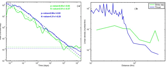
I show, average values of different spatio-temporal parameters (rate, p, K − value and H) are dependent on faulting styles. Thrust events have higher diffusion, rate, duration and background rate as compare to strike slips events. Higher duration in the environment of high background rate is driven by high branching ratio and low p − value of thrust events as compare to that of strike slip. For normal events to limited data we only analysis its p − value. Which has highest p − value as compare to other faulting styles. Density rate diffusion of thrust events are different as compare to strike slips events, which further implies different diffusion of faulting styles. This work has been submitted in Journal of Geophysical Research.

In chapter 3, we analyse largest aftershock patterns. Average magnitude ∆M, time ∆T

and normalize distance ∆D∗ _{between mainshock and its corresponding largest aftershock}

is independent of mainshock magnitude. The largest aftershock is bounded on average by -1.2 magnitude from the mainshock. Thirty years of the global earthquake catalogue allow

us to extend B˚ath’s law in the time and space domains, as the largest aftershocks are closer

in size (mode value : ∆Mr = 0.95, ∆Mss = 1.51) and distance (mode value : ∆Dr∗ = 0.11,

∆D∗

ss = 0.22) to the triggering shock, for (r) reverse slip than for (ss) strike slip events.

The faster power law decay in time relative to regular aftershocks implies that the largest aftershocks are more prone to occur at the onset of any aftershock sequence. This pattern is the only to be reproduced by a branching point model. This work has been submitted in GeophysicalResearchLetters.

In chapter 4, We analysis spatio-temporal parameters of the global stacked data.

Af-tershocks productivity increases with that of mainshock magnitude ∼ 10αm_{, with α = 0.82}

± 0.06. p − value is a function of mainshock magnitude for direct aftershock, whereas correlation is lost when we have both direct and indirect aftershock. Duration has a posi-tive correlation with mainshock magnitude. Stress step and duration decreases as distance from mainshock increases. We also observed that linear density obeys power law and its peak density distance from the mainshock is dependent on mainshock size. We resolve

static stress triggering is the main responsible mechanism for global earthquake triggering process. This work has been submitted in Journal of Geophysical Research.

In chapter 5, We analyzed Omori’s law exponent (p − value from N(t) = K

(t+c)p) and

diffusion exponent (H from R(t) = tH_{) of foreshocks and aftershocks. p − value of the}

stack aftershocks is higher than that of the foreshocks, whereas the same pattern observed for the decay slope of linear density.

Previously, earthquake scale invariance are shown either in space or in time. But lim-ited or negligible work has done on scale invariance of both time and space. This link between space and time would help us in better understanding the triggering mechanism of the fault systems. We observe that seismicity rate (number/km/day) as a function of

distance obey as power law (Φ(t) ∼ 1

(d+r)1+µ). The exponent µ decreases and finally reaches

to the background level at long time (> 2000 day) window with µ ∼ 0. Aftershocks density rate (number/km/day) expansion toward the background is slower as compare to the fore-shocks inverse expansion (from background toward the mainshock). Initially (upto 5 days),

aftershocks migrate slowly away from the mainshock than that of the foreshocks (Haf t. =

0.07 and Hf ore. = 0.20). But for time (> 5 days) contemporary to the occurrence of largest

aftershock, the migration of aftershocks becomes fast (Haf t. = 0.38). Linear density show

aftershock diffusion that is different from that of foreshock, whereas background have nearly same value of the exponent. This work will be submitted in GeophysicalResearchLetters.

Les grands s´eismes et leurs r´epliques sont une menace pour la soci´et´e et les ˆetres hu-mains. Ils sont rares en raison de leur faible r´ecurrence, mais la plupart d’entre eux sont tr`es dangereux, causant environ 50 pour cent de la perte totale dans des la vie humaine et 30 pour cent des pertes ´economiques au cours des 50 derni`eres ann´ees (Woessner and Wiemer (2005)). Le s´eisme d’octobre 2005, au Cachemire a gravement endommag´e les ter-res cultivables, les infrastructuter-res physiques, l’infrastructure sociale, la fourniture de biens publics, la qualit´e de l’eau et ses sources, les sys`eteme d’assainissement et d’´egouts, de sant´e et de nutrition dans l’Azad Jammu et Cachemire et la zone nord du Pakistan. Les pertes ´economiques totales dues `a des dommages et des destructions sont estim´ees `a environ 5 milliards dollars am´ericains (Maqsood and Schwarz (2010)). Plus de 73,000 personnes ont perdu la vie, et 128 000 personnes ont ´et´e bless´ees lors du s´eisme (selon l’Autorit´e nationale de gestion des catastrophes du Pakistan (NDMA 2007), http://ndma.gov.pk).

Les scientifiques, les ing´enieurs et les autorit´es sont responsables pour att´enuer le risque sismique afin de r´eduire les pertes humaines et financi`eres `a l’avenir. Le plus important d’un point de vue scientifique, est de comprendre la physique du tremblement de terre, son m´ecanisme de d´eclenchement et de mettre en œuvre des mod`eles de risque. Pour contribuer `a ces efforts scientifiques dans les mod`eles de risque, les m´ethodes statistiques bas´ees sur l’analyse spatio-temporelle de la sismicit´e en champ proche donnent acc`es un le lien entre la physique et le m´ecanisme de d´eclenchement du tremblement de terre, pouvant en outre ˆetre utilis´e dans les mod`eles de pr´evision des s´eismes.

concentrons sur le m´ecanisme de d´eclenchement du tremblement de terre en consid´erant les grands tremblements de terre et leurs r´epliques en essaim, ces devenirs parfois posent plus de risques que le choc principal, en raison de leur large gamme de fr´equences, de leurs diff´erentes tailles et du fait leur grand nombre en peu de temps (e.g., Reasenberg and Ellsworth (1982); Okubo and Aki (1987)). Les questions principales lois de cette recherche ont ´et´e;

• quel param´etres contrˆole la prodcutivit´e spatio-temporelle des r´epliques? • comment les r´epliques d´ependent elles du type de failles?

• Quand, `a quelle distance et o´u les plus fortes r´epliques se produisent-elles? • est-ce que la plus grande r´eplique contrˆole les r´egimes de diffusion?

• y at-il une d´ependance ´a la magnitude de p, de α, de la dur´ee de et l’h´et´erog´en´eit´e des contraintes.

• est-ce quelle le d´eclenchant des r´eliques est contrˆol´e principalement par un m´ecanisme statique ou dynamique?

Les tremblements de terre sont la r´eponse cassante de la croˆute terrestre `a des

con-traintes appliqu´ees (e.g., Lee (2003); Rundle et al. (2003)). Les d´eformations significatives sont n´ecessaires pour d´evelopper une fracture dans l’environnement fragile (Lee (2003)). Les d´eformations `a travers ces fractures g´en`eres des h´et´erog´en´eit´e d´efauts (Lee (2003)).

Manifestement, ces tailles ou ces fractures dans la croˆute terrestre sont complexes et se

produisent sur une large gamme d’´echelles (e.g., Mandelbrot (1983)). En g´en´eral, les r´egions sismiquement actives sont d´ecoup´ees par un certain nombre de r´eseaux de failles, qui pr´esentent des statistiques fractales tant dans la distribution de rugosit´e de surface et dans leur distribution de longueur (e.g., Okubo and Aki (1987)). Kagan (1993) sugg`ere en outre que les s´eismes se produisent sur les structures fractales de nombreuxs failles ´etroitement li´ees plutˆot que sur une faille unique. Une approche pour l’analyse des trem-blements de terre est de supposer les glissments et les d´eplacements sur une faille active

unique dans une r´egion plutˆot que de consid´erer toutes les failles. Sous cette hypoth`ese, les gros s´eismes sur la faille principale se produisent sur une base p´eriodique et la p´eriode durant laquelle il n’y a aucun tremblement de terre est appel´ee lacune sismique. Une

ap-proche alternative `a la m´ecanique du tremblement de terre est de supposer que la croˆute

est un syst`eme complexe auto-organis´e qui peut ˆetre trait´e par des techniques statistiques (e.g., Lee (2003)).

Les r´epliques sont couramment observ´ee apr`es chaque grand tremblement de terre. G´en´eralement chaque tremblement de terre interagit avec d’autres structures en appli-quant certaines charges sur les failles voisines et lointaines, qui cassent. La relaxation des contraints tectoniques est donc complexe et implique de grands ensembles de tremblements de terre de taille diff´erente, sur l’´echelle spatiale et temporelle (Marsan (2003)). De nom-breux mod`eles physiques ont ´et´e propos´es pour expliquer le processus de d´eclenchement des tremblements de terre (e.g., Scholz, 1968; Nur and Booker, 1972; Stein and Lisowski, 1983; Oppenheimer et al., 1988; Mendoza and Hartzell, 1988; Reasenberg and Simpson, 1992b; Stein et al., 1992; King et al., 1994; Boatwright and Cocco, 1996; Stein et al., 1997; Dieterich, 1994; Gomberg et al., 1998; Harris, 1998; Kagan and Jackson, 1998; Stein, 1999; Toda et al., 1998; Gomberg et al., 2000; Toda and Stein, 2000; Freed and Lin, 2001; Gomberg et al., 2001b; Kilb et al., 2002; Helmstetter et al., 2002; Steacy et al., 2005; Toda et al., 2005).

G´en´eralement le m´ecanisme de d´eclenchement des r´epliques a ´et´e mod´elis´e en utilisant soit le calcul de transfert de contrainte statique, dans lequel les r´epliques se produisent dans la zone des changements positifs de la contrainte co-sismique (King et al., 1994; Stein, 2003), ou comment un processus dynamique de d´eclenchement dynamique, caus´ee par le passage des ondes sismiques (Voisin, 2002; Perfettini et al., 2003), ou par la relaxation due aux effets visco´elastiques (Romanowicz, 1993; Piersanti et al., 1995, 1997; Zeng, 2001), ou le mod`ele de friction de rate and state ((Dieterich (1994)), et la rh´eologie (Ben-Zion and Lyakhovsky (2006)). Ainsi, `a courte ´echelle de temps, `a la fois les changements des contraintes dynamiques et statiques sont tr`es importants tandis que `a grande ´echelle les changements visco´elastiques peuvent conduire `a l’occurrence de tremblements de terre

temporellement retard´ee. D’autres facteurs comme le type de rupture et de glissement de petites h´et´erog´en´eit´e d’´echelle peuvent aussi avoir un effet sur la distribution des s´eismes (e.g., Marsan (2006)).

Le d´eclenchement d’un grande s´eisme peut arriver rapidement, comme dans le cas du Big bear earthquake, suivant seulement d’une heure le tremblement de terre ”Lander” (e.g., Pollitz and Selwyn Sacks (1997); Freed (2005)). En raison de cette complexit´e, il ya un besoin ´evident en physique du tremblement de terre d’observations plus int´egratives, de mod´elisation et d’analyses statistiques. Comprendre les mod`eles de d´eclenchement va nous aider `a d´eceive la physique du cycle de tremblements de terre et, surtout, peut grandement

aider notre capacit´e d’att´enuation des risques sismiques en pointant la zone o`u le prochain

grand tremblement peut se produire (e.g., Freed (2005)). Les mod`eles bas´es sur la physiques sont utiles pour comprendre les processus physiques, tandis que les mod`eles statistiques du tremblement de terre peuvent ˆetre tr`es utiles pour extraire des dans les domain taille, space et temp.

L’interd´ependance des param`etres spatio temporelles des r´epliques et de ses change-ments syst´ematiques avec diff´erentes tectoniques a ´et´e observ´ee dans de nombreuses ´etudes (e.g., Wiemer and Katsumata, 1999; Schorlemmer et al., 2005; Narteau et al., 2009; Peixoto et al., 2010). Bas´e sur ces r´esultats, j’ai consacr´e une grande partie de mon travail de th`ese `a d´evelopper certaines corr´elations spatio-temporelles des param`etres de r´epliques pour tester leur d´ependance `a l’angle de glissement et `a la nature du m´ecanisme de d´eclenchement.

La motivation principale du chapitre 1 est de trouver r´eponses pour les productions des r´epliques les plus ´elev´ees du tremblement de terre du Cachemire en 2005, compar´e aux

grandes s´equences de r´epliques (Mm ≥ 7.0) survenues a pr`es de 20◦ autour de l’´epicentre

du tremblement de terre du Cachemire. Les taux normalis´es, la dur´ee, les param`etres de la loi d’Omori et la densit´e moyenne de 18 s´equences de r´epliques, ont ´et´e calcul´es. Les corr´elations entre ces param`etres ont ´et´e test´ees, quand il ya un d´ebat ouvert sur ces su-jets. En revanche Marsan and Lengline (2008) ont observ´e que la dur´ee de la s´equence de r´epliques est tr`es bien corr´el´ee avec la taille du choc principal. Drakatos and Latoussakis (2001) r´esolvent une corr´elation similaire entre la dur´ee des r´eliques et la taille du choc

prin-cipal en utilisant des donn´ees de Gr`ece. Des d´ependances des param`etres spatio-temproal aux styles de failles sont ´egalement observ´ees, bien que nous utilisions 18 s´equences de r´epliques, qui consistent en quatre coulissage, 13 faille inverse et 1 ´ev´enement en faille normale. Ce travail a ´et´e pr´esent´e dans le Bulletin of the Seismological Society of America.

Dans le chapitre 2, j’applique le rˆole styles de failles `a comme observ´e pour les petits volumes de donn´ees dans le chapitre (1) des donn´ees `a l’´echelle mondiale. Schorlemmer et al. (2005) montrent que la b − valeur est d´ependante du type de faille, en utilisant la Californie et des donn´ees mondiales. De la mˆeme mani`ere Gulia and Wiemer (2010) utilisent des donn´ees d’Italie montrent et que la taille du tremblement de terre d´epend du orientation du glissement sismique. Narteau et al. (2009) montrent que la valeur c est d´ependante du rake de langle d’inclinaison de la faille. Il n’existe pas de mod`ele pour la production des r´eplique, la valeur p et le taux de r´elique. Comme la valeur b, la p − valeur est ´egalement fortement affect´ee par le m´ecanisme de relaxation les contraintes et des lois de friction dans la zone sismog´ene (Mikumo and Miyatake (1979); Dieterich (1986)).

Je montre que les valeurs moyennes des diff´erents param`etres spatio-temporels (taux, p, K et H) sont d´ependants des types de failles. Des ´ev´enements en faille inverse ont une dur´ee, un taux, une sismicit´e de fond et une diffusion plus ´elev´es, compar´e aux ´ev´enements en coulissage. Les plus grandes dur´ees dans un environnement de bruit de fond ´elev´e sont contrˆoll´ees par le fort rapport de branchement et la faille valeur p des ´ev´enements en faille inverse compar´e ´a des coulissage. La diffusion du taux de densit´e d’´ev´enements en faille inverse est diff´erente de celle des ´ev´enements coulissage, ce qui implique en outre des diffusions diff´erent suivant le type de faille. Ce travail a ´et´e soumis au Journal of Geophysical Research.

Dans le chapitre 3, nous avons analys´e les mod`eles des plus grandes r´epliques. La

mag-nitude moyenne ∆M, le temps ∆T et la distance normalis´ee ∆D∗ _{entre le choc principal}

et sa plus grande r´eplique sont ind´ependant de la magnitude du choc principal. La plus grande r´eplique est limit´ee en moyenne `a -1.2 de la magnitude du choc principal. Trente

domaines du temps et de l’espace, car les plus grande r´epliques sont plus proches en taille

(valeur mode: ∆Mr = 0.95, ∆Mss= 1.51) et distance (valeur en mode: ∆D∗r = 0.11, ∆D∗ss

= 0.22) du choc de d´eclenchant, pour (r) un glissement inverse que pour des ´ev´enements

en coulissage(ss). La d´ecroissance rapide de la loi puissance dans le temps par rapport aux

r´epliques r´eguli`eres implique que les plus grandes r´epliques sont plus probable au d´ebut de n’importe quelle s´equence de r´epliques. Cette observation est le seule `a ˆetre reproduite par un mod`ele de point de branchement. Ce travail a ´et´e pr´esent´e dans Geophysical Research Letters.

Dans le chapitre 4, nous faisons une analyse spatio-temporelle des param`etres des donn´ees globales stack´ees. La productivit´e de r´epliques augmente avec la magnitude du

choc principal ∼ 10αm_{, avec α = 0.82 ± 0.06. La valeur p est fonction de la magnitude du}

choc principal pour les r´epliques directes, alors que la corr´elation est perdue lorsque nous avons `a la fois des r´epliques directes et indirectes. La dur´ee a une corr´elation positive avec la magnitude du choc principal. Nous avons ´egalement observ´e que la densit´e lin´eaire ob´eit `a la loi de puissance et que la distance de son pic de densit´e au choc principal d´epend de la taille du choc principal. Nous sugg´erons que le d´eclenchement par la contrainte statique est le principal m´ecanisme responsable des processus de d´eclenchement des tremblements de terre mondiaux. Ce travail a ´et´e soumis au Journal of Geophysical Research.

Dans le chapitre 5, nous avons analys´e l’exposant de loi d’Omori (p − valeur de N(t) =

K

(t+c)p) et la diffusion de l’exposant (H de R(t) = tH) pour des pr´ecurseurs et des r´epliques.

La valeur p des r´epliques stack´ees est plus ´elev´ee que celle des pr´ecurseurs, alors que le mˆeme sch´ema est observ´e pour la pente de la d´ecroissance de densit´e lin´eaire.

Auparavant, l’invariance d’´echelle du tremblement de terre a ´et´e indiqu´ee dans l’espace ou dans le temps. Le lien entre l’espace et le temps peut nous aider `a mieux comprendre le m´ecanisme de d´eclenchement des syst´emes de failles. Nous observons que le taux de sismicit´e (nombre / km / jour) en fonction de la distance ob´eit `a une loi de puissance

(H(t) ∼ 1

(D+R) 1+µ

). L’exposant µ diminue et atteind le niveau de fond `a long terme (> 2000 jours) avec µ ∼ 0. L’expansion de taux de densit´e de r´epliques (nombre / km / jour) vers le niveau de fond est plus lent compar´e `a la contraction des pr´ecurseurs (`a partir du

niveau de fond vers le choc principal). Initialement (jusqu’`a 5 jours), des r´epliques migrent

plus lentement ´a partir du choc principal que pour les pr´ecurseurs (Haf t. = 0.07 et de Hf ore.

= 0.20). Mais pour le temps (> 5 jours) contemporain de l’apparition de la plus grande

r´eplique, la migration des r´epliques devient rapide (Haf t. = 0.38). La diffusion lin´eaire des

r´eplique est diff´erente de celle des pr´ecurseurs, alors que la sismicit´e de fond `a presque la mˆeme valeur dans les 2 cas. Ce travail sera pr´esent´e dans Geophysical Research Letters.

Aftershocks patterns in the Asian

continental collision belt and the

Muzafffarabad, Kashmir, 2005,

sequence.

M. Tahir 1_{, JR Grasso}1

1_{Institut des sciences de la Terre (ISTerre)}

University Joseph Fourier - Grenoble I, FRANCE

Abstract

The seismicity rate triggered by the Muzaffarabad, Kashmir, 2005 Mw = 7.6,

Ms= 7.7 earthquake appears as above the average when analysing the aftershocks sequences

in the India-Asia collision belt for period of 1973-2008. To quantify this pattern we

com-pare the aftershock patterns triggered by the 18 Ms ≥ 7.0 earthquakes which occurred in

20◦ _{latitude and 40}◦ _{longitude box size, centered on the Muzaffarabad (Kashmir, 2005)}

earthquake epicenter. Such area, stands as the major region in which continental plates interact, worldwide. After normalizing by the mainshock size and by the magnitude range

of observation, the Ms = 7.7 Kashmir, the Ms = 7.0 Khurgu (Iran, 1977) and the Ms= 7.6

Southern Xinjiang (China, 1985) aftershocks rates are above the 1-2 standard deviations of the 18 aftershocks rates. We test how Omori’s law parameters, background rate, space and time patterns of the sequences interplay to produce the huge aftershock productivity for Kashmir earthquake. This anomaly of Kashmir sequence rate is not driven by a single Omori law parameter. It appears as a combination of many parameters that leads to a relatively longer sequence duration, higher density, in a higher background rate setting (pre stress conditions) than the others western Asia sequences, respectively. For the Khurgu Iran sequence, the anomaly in large rate emerges as driven by a large aftershocks produc-tivity, as measured from the normalized K − value of the Omori law. Also this aftershock cascade develops further away in space, above a two standard deviation significance level, than for the other sequences respectively. Normalization by earthquake sizes allow us to identify anomalies in aftershock sequence, i.e. above two times of standard deviation, for the productivity and rate of Khurgu earthquake, aftershock density for Kashmir sequences, high background rate for Southern Keriya sequence and long duration for Gazli (1976b) and Qaenat earthquakes. The other major result we robustly quantify for Western Asia

Ms >7.0 events, is the dependence of aftershock productivity on faulting styles, for all of

the Omori law parameters. We resolved the strike slip event productivity to be on average 4 times smaller than the thrust faulting productivity.

Les taux normalis´es, la dur´ee, les param`etres de la loi d’Omori et la densit´e moyenne de 18 s´equences de r´epliques, ont ´et´e calcul´es. Les corr´elations entre ces param`etres ont ´et´e test´ees, quand il ya un d´ebat ouvert sur ces sujets. En revanche Marsan and Lengline (2008) ont observ´e que la dur´ee de la s´equence de r´epliques est tr`es bien corr´el´ee avec la taille du choc principal. Drakatos and Latoussakis (2001) r´esolvent une corr´elation similaire entre la dur´ee des r´eliques et la taille du choc principal en utilisant des donn´ees de Gr`ece. Des d´ependances des param`etres spatio-temproal aux styles de failles sont ´egalement observ´ees, bien que nous utilisions 18 s´equences de r´epliques, qui consistent en quatre coulissage, 13 faille inverse et 1 ´ev´enement en faille normale.

1.1

Introduction

The Muzaffarabad earthquake, October, 8th 2005, Kashmir, Pakistan, Mw =

7.6 is one of the rare, if any, Himalayan quakes that produced a surface faulting in the past centuries (Avouac et al. (2006); Grasso and Mughal (2006); Pathier et al. (2006)). It was followed by relatively large number of aftershocks, as compare to the other mainshock

(Ms ≥ 7.0) situated in the Indian-Asia collision belt (figure 1.1). The aftershock activity

was particularly intense beyond the NW termination of the fault rupture (Avouac et al.

(2006)). The largest aftershock with magnitude (Mw = 6.5) occurred on December 12th

2005 and located (latitude = 36.36N, longitude = 71.09E) ∼ 305 km from the mainshock

location. The second largest aftershock with magnitude (Mw = 6.4) occurred on the same

day of the mainshock and located (latitude = 34.73N, longitude = 73.10E) very close (∼ 50 km) to the mainshock location. The difference between Kashmir mainshock and its

largest aftershock magnitude obeys B˚ath’s law i.e., ∆M = 1.2. We aim to quantify and

to understand the specificity of the Muzaffarabad earthquake sequence, by comparing the

aftershock spatial and temporal patterns of this event to the one of Ms ≥ 7.0 events in

the surrounding regions. In particular, we seek a physically based relationship between the causative faulting parameters and the aftershocks density in space and time.

stress-strain rate changes triggered by any given earthquake. Because aftershocks exist for every earthquake, it is suggested by this property to go beyond the a-priori defini-tion of foreshock-mainshock-aftershock time dependance as condidefini-tioned on the earthquake size (e.g., Helmstetter et al. (2002); Helmstetter and Sornette (2003a)). It is suggested that aftershocks production depend on rock type, ambient temperature and fluid content ( Ben-Zion (2008); Yang and Ben-Zion (2009)). Previous studies show that cold continen-tal regions have high aftershock productivity and long duration of aftershock sequences, whereas hot continental regions and oceanic lithosphere have low aftershock productivity and short sequence (e.g., Mogi (1967); Davis and Frohlich (1991); Kisslinger and Jones (1991); Utsu et al. (1995); McGuire et al. (2005)).

In the near field, i.e., within a couple of fault length from the trigger shock, the seismic rate globally increases where the co-seismic stress change, i.e., the Coulomb Stress Change, is positive ( Mendoza and Hartzell (1988); Boatwright and Cocco (1996); Stein et al. (1997); Gomberg et al. (1998); Harris (1998); Stein (1999); Gomberg et al. (2000); Toda and Stein (2000); Kilb et al. (2002)). Because of the few bar changes that are resolved to increase the seismicity rate after each given shock, aftershocks are suggested as triggered slips on faults that are already close to instability threshold (Console and Catalli (2005); Ziv (2006a)). Thus in the near field i.e., 1-3 fault length, the static stress change is suggested to drive the aftershock triggering (e.g., Parsons et al. (2006); Hainzl et al. (2010b)). At large distances static stress changes is suggested to be too low to trigger aftershocks (e.g., Hill et al. (1993)) then the distant triggered slips could be related to the dynamic stress changes (Freed (2005); Felzer and Brodsky (2006)).

Reasenberg and Simpson (1992a) show that the aftershocks production rate are depen-dent on the background rate with using the seismicity rate changes in central California occurring at the time of Loma Prieta earthquake. Similarly Toda et al. (2005) used south-ern California data for period of 1986-2003, suggest that background seismicity is the key parameter for the aftershock production, coulomb stress changes efficiently being ampli-fied by the background seismicity. These authors validated this model by using Big Bear, Barstow and Hector Mine seismicity which became active immediately after the Landers

earthquake despite experiencing only small static stress increases. Accordingly, small stress changes are suggested to produce large changes in the seismicity rate in the areas of high background seismicity (Toda et al. (2005)). Following Dieterich (1994) using rate and state friction law, the seismicity and background rate are linearly proportional and simi-lar scaling exists between aftershock production and stress step. When the stress step is high, the higher will be the aftershock production and vice versa. The rate of production of earthquake changes through time after a stress step is reproduced by a rate and state friction law (Dieterich (1994)). In this model, the duration of the aftershock sequence, i.e., the time when the aftershock rate decline down to the background seismcity rate, is a characteristic feature of earthquake recurrence time. Dieterich model further shows that aftershock duration is stress step dependent (Dieterich, 1994). Drakatos and Latoussakis (2001) show for aftershock sequences in Greece (1971–1997) that duration and magnitude have correlation even though their residual square is poor, i.e., 30%. In a similar way Marsan and Lengline (2008) show that duration and aftershock production is very well correlated with mainshock magnitude for dressed (direct + indirect) aftershock sequence. Kagan (2002a) correlates the size of aftershock zone with mainshock magnitude (≥ 7.0) using global data, aftershocks being defined as events that occur within 7 days after the mainshock.

In this study we made an attempt toward a comprehensive analysis of aftershocks

patterns in space and time for the Kashmir events as compared to the others 17 Ms ≥ 7

events occurring within thousand kilometer square on the 1973 - 2008 period and centered at the 2005 Kashmir event. We first normalized the aftershock production rate by the mainshock sizes and catalogue completeness. Using these normalized data allows us to cross analyse the density, the rate, the duration and the size of aftershock zone for 18 aftershock sequences. We correlate these parameters with the one of the Omori law, the background rate and the mainshock faulting style. We extract earthquake outliers as event for which parameters are above or below 1-2 standard deviations, as computed for the values of 18 sequences, respectively. Finally we discuss the physical processes that are possible candidates to reproduce the observation.

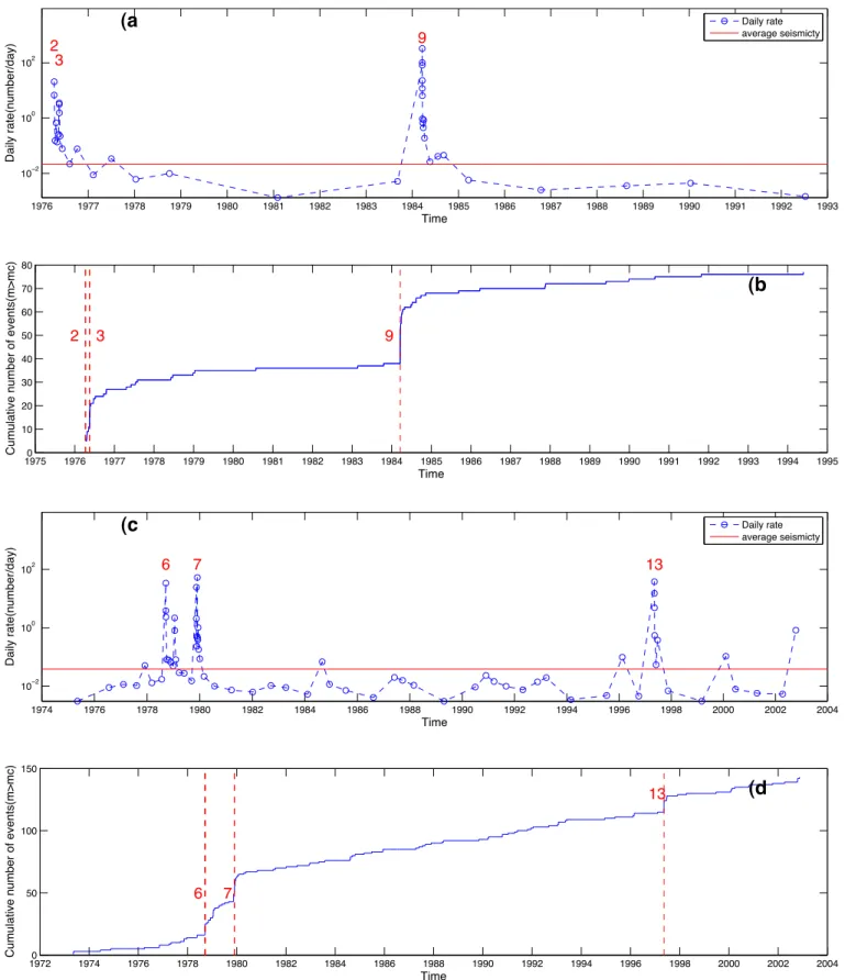
19730 1975 1977 1979 1981 1983 1985 1987 1989 1991 1993 1995 1997 1999 2001 2003 2005 2007 20 40 60 80 100 120 140 160 180 Time(year) Daily rate(number/day) ↓ ↓↓ ↓ ↓ ↓ ↓ ↓ ↓ ↓ ↓ ↓ ↓ ↓ ↓ ↓ ↓ ↓ 7.3 6.6 6.7 6.7 6.9 7.3 7 7.2 7 6.9 7.2 7.1 7.2 7.5 7.67.8 7.6 7.1 1 2 3 4 5 6 7 8 9 10 11 12 13 14 1516 17 18 Seismicity Background

Figure 1.1: Daily seismicity rate, within ± 10◦ _{(latitude) and ± 20}◦ _{(longitude), box}

centered on Kashmir earthquake. Black numbers show the sequence number (table

2.1) and red numbers are mainshock magnitude (Mw). Data are taken from USGS

(http://earthquake.usgs.gov)

1.2

Mainshocks and Aftershocks selection

We have selected Ms ≥ 7.0 earthquakes that are located within 10◦ of

lati-tude and within 20◦ _{longitude relatively to the Muzaffarabad, October 8}th ₂₀₀₅

epicen-ter. Such a box, centered on Kashmir 2005 earthquake, stands as the major region in which continental plates interact, worldwide (figure 1.2). The data we use are from USGS (http://earthquake.usgs.gov) and global harvard CMT catalogs

(http://www.globalcmt.org-/CMTsearch.html). For the 18 (Ms ≥ 7.0) earthquakes in the study area we use as

main-shocks, there are large fluctuations between Ms and Mw (figure 1.3, table 2.1).

We used [± 5 yr, 5L] window from the mainshock, to estimate the mc completeness

value of each sequence. The fault length (L) for each event is estimated using Wells and Coppersmith (1994) formula. Then, we impose the aftershock magnitudes to be larger than

the completeness mc value, this later being estimated for each sequence by using maximum

curvature technique (Wiemer and Wyss (2000); Woessner and Wiemer (2005)) (figure 1.4, table 1.2). We tested the results are stable on [1, 5, 10]*L set of normalized aftershock

distances to the mainshock. On the 18 aftershocks sequences from Ms ≥ 7.0, 1973-2008,

One of these events, the Kulun Shan, 2001 earthquake is suggested to have a supershear rupture velocity (Bouchon and Vall´ee (2003)). This later appears to trigger aftershocks at larger distance from the mainshcoks epicenter and to have only few aftershocks in the epicentral region relatively to the other events (Bouchon and Karabulut (2008)).

60˚ 60˚ 70˚ 70˚ 80˚ 80˚ 90˚ 90˚ 20˚ 20˚ 30˚ 30˚ 40˚ 40˚ 60˚ 60˚ 70˚ 70˚ 80˚ 80˚ 90˚ 90˚ 20˚ 20˚ 30˚ 30˚ 40˚ 40˚ (8/1974)7.3 1 (4/1976)6.6 2 (5/1976)6.7 3 (3/1977)6.7 4 (3/1978)6.9 5 (6/1978)7.3 6 (11/1979)7.0 7 (7/1981)7.2 8 (3/1984)7.0 9 (8/1985)6.9 10 (8/1992)7.2 11 (2/1997)7.1 12 (5/1997)7.2 13 (11/1997)7.5 14 (1/2001)7.6 15 (11/2001) 7.8 16 (10/2005)7.6 17 (3/2008)7.1 18 Kashmir Khurgu

Tabas block Lut block

Zagros

Indian shield

Tibetan plateau Tien Shan(Tarim)

Mainshock Seismicity (M >= 4.7) 6.5 <= M <7.0 7.0 <= M <=7.5 M > 7.5

Figure 1.2: Shallow earthquakes with magnitude greater than threshold

magnitude(mc ≥4.7) red circle are mainshocks (Ms ≥7.0). Red lines are major

faults in the area (Peltzer and Saucier (1996);Hatzfeld and Molnar (2010);Replumaz (1999)). All blue labels are major tectonic blocks (Hatzfeld and Molnar (2010)).

6.5 6.7 6.9 7.1 7.3 7.5 7.7 7.9 6.5 6.7 6.9 7.1 7.3 7.5 7.7 7.9 Magnitude(M w) Magnitude(M s ) M s=0.84*Mw + 1.41 1 2 3 4 5 6 8 9 10 11 14 15 16 17 18 7 13 12 R s=0.76

Figure 1.3: Ms (surface wave magnitude) versus Mw (moment magnitude) of 18 major

events (Ms ≥ 7.0) of the Eurasia collision zones with time period of 1973-2008. 1 normal

event (red), 13 thrust (blue) and 4 strike slip (green) events are seleceted. Events number are from table 2.1.

Num Name Date _MMagnitude Location Mech Depth(km) L(km) Surface

s Mw Longitude Latitude Rupture(km)

1 Markansu,Tajikistan 11/08/1974 7.3 7.1 73.83 39.46 Thrust 9 65.6 NI

2 Gazli, Uzbekistan 08/04/1976 7.0 6.6 63.77 40.31 Thrust 33 21.6 No

3 Gazli, Uzbekistan 17/05/1976 7.0 6.7 63.47 40.38 Thrust 10 25.3 No

4 Khurgu, Iran 21/03/1977 6.9 6.7 56.39 27.61 Thrust 29 25.3 No

5 Zhalanash Tyup, Kazakhstan 24/03/1978 7.1 6.9 78.61 42.84 Thrust 33 34.8 NI

6 Tabas, Iran 16/09/1978 7.4 7.3 57.43 33.39 Thrust 33 65.6 85 km1

7 Ghanenat(Qaenat), Iran 27/11/1979 7.1 7.0 59.73 33.96 Strike Slip 10 40.7 60 km2

8 Sirch(Kerman), Iran 28/07/1981 7.1 7.2 57.79 30.01 Thrust 33 56.0 5 km3

9 Gazli, Uzbekistan 19/03/1984 7.0 7.0 63.35 40.32 Thrust 14 40.7 NI

10 Southern Xinjiang, China 23/08/1985 7.6 6.9 75.22 39.43 Thrust 6 34.8 NI 11 Susamyr, Kyrgyzstan 19/08/1992 7.4 7.2 73.57 42.14 Thrust 27 56.0 50 km4

12 Quetta, Pakistan 27/02/1997 7.3 7.1 68.21 29.98 Thrust 33 47.8 NI

13 Qaenat, Iran 10/05/1997 7.3 7.2 59.81 33.83 Strike Slip 10 56.0 150 km5

14 Mani, China 08/11/1997 7.9 7.5 87.32 35.07 Strike Slip 33 90.2 NI

15 Bhuj, India 26/01/2001 8.0 7.6 70.23 23.42 Thrust 16 105.7 NO

16 Kulun shan, China 14/11/2001 8.0 7.8 90.54 35.95 Strike Slip 10 145.2 400 km6

17 Kashmir, Pakistan 08/10/2005 7.7 7.6 73.59 34.54 Thrust 26 105.7 70 km7 18 southern Keriya, China 20/03/2008 7.3 7.1 81.47 35.49 Normal 10 47.8 NI Ms=Surface wave Magnitude

Mw= Moment Magnitude

NI = No information available NO= No Surface rupture observed Mech=Mechanism

L=Rupture length calculated from Wells and Coppersmith (1994) Surface Rupture = Surface rupture reported in literature

1

Berberian (1979),2

Haghipour and Amidi (1980),3

Adeli (1982),4

Ghose et al. (1997),5

Berberian and Yeats (1999),6

Lin et al. (2002),7

Kaneda et al. (2008),

Table 1.1: Mainshocks parameters

1.3

Analysis of aftershock patterns in time and space

1.3.1

Normalised aftershock rate

The number of aftershocks (m ≥ mc) for each of the mainshock were calculated using a

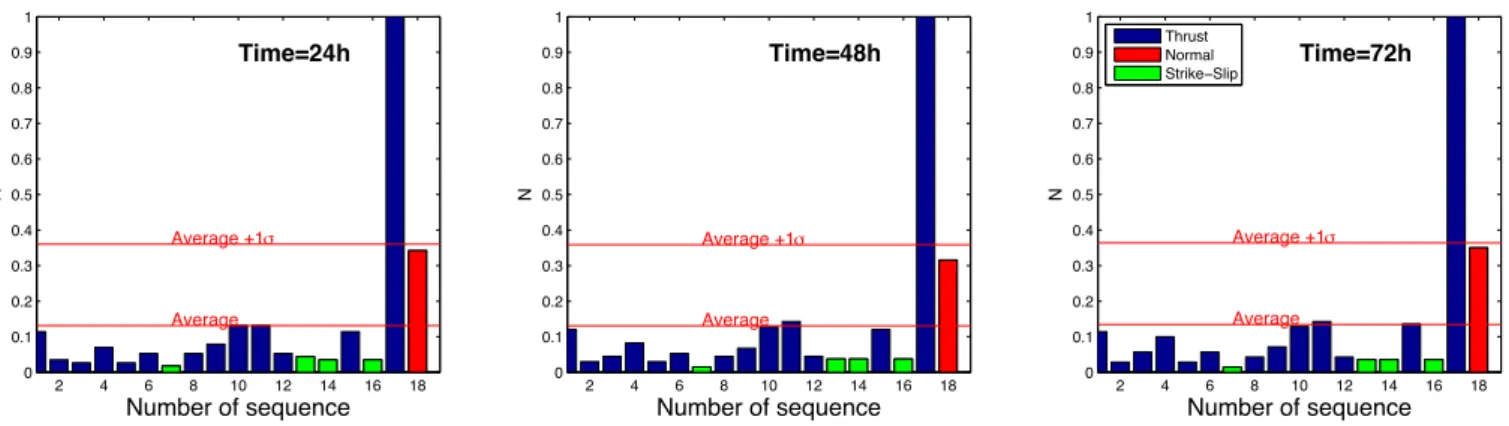
fixed distance, 5*L (L is fault length calculated from Wells and Coppersmith (1994)) and time window as 24, 48 and 72 hours after the mainshock, respectively. These time windows allow to withdraw any possible finite size effect induced by the difficulty to pinpoint the onset and the end of the aftershocks sequence. The relative ranking of daily rate produc-tivity of the 18 events are stable for 24, 48 and 72 hours respectively (figure 1.5). Always the Kashmir sequence is the most productive. The same analysis is repeated for 1*L and

10*L, but the results are still stable. Number of aftershocks n(mm) of a mainshock of

magnitude (mm) is proposed as;

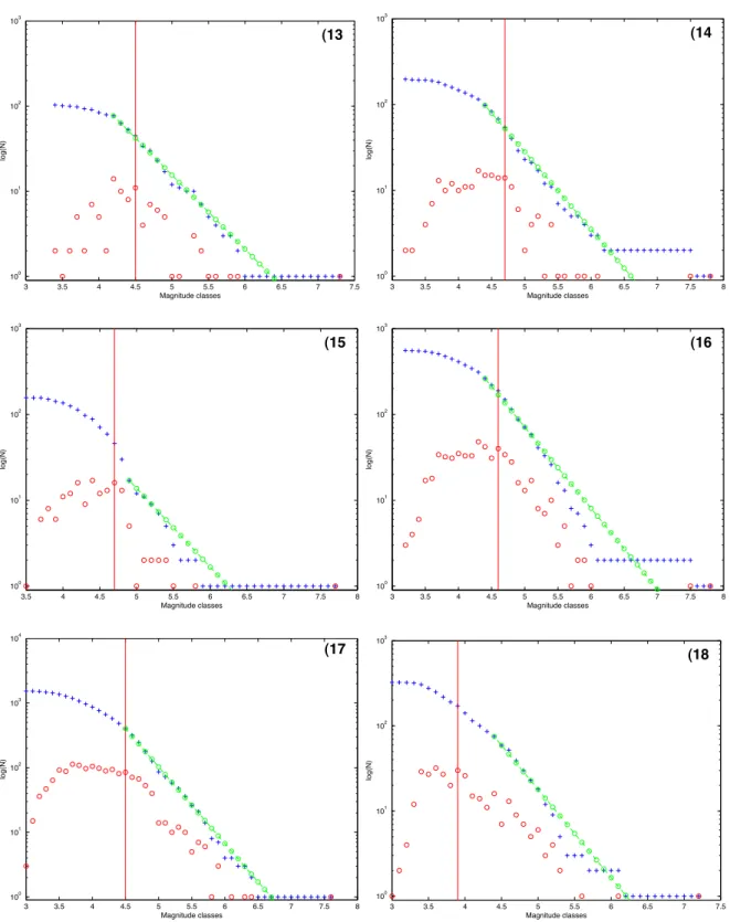
3.5 4 4.5 5 5.5 6 6.5 7 7.5 100 101 102 103 Magnitude classes log(N) (1 3.5 4 4.5 5 5.5 6 6.5 7 7.5 100 101 102 Magnitude classes log(N) (2 3.5 4 4.5 5 5.5 6 6.5 7 7.5 100 101 102 Magnitude classes log(N) (3 3.5 4 4.5 5 5.5 6 6.5 7 100 101 102 103 Magnitude classes log(N) (4 3.5 4 4.5 5 5.5 6 6.5 7 7.5 100 101 102 Magnitude classes log(N) (5 3 3.5 4 4.5 5 5.5 6 6.5 7 7.5 8 100 101 102 103 Magnitude classes log(N) (6

3.5 4 4.5 5 5.5 6 6.5 7 7.5 100 101 102 Magnitude classes log(N) (7 4 4.5 5 5.5 6 6.5 7 7.5 100 101 102 103 Magnitude classes log(N) (8 4 4.5 5 5.5 6 6.5 7 7.5 100 101 102 Magnitude classes log(N) (9 3.5 4 4.5 5 5.5 6 6.5 7 7.5 100 101 102 103 Magnitude classes log(N) (10 3.5 4 4.5 5 5.5 6 6.5 7 7.5 100 101 102 103 Magnitude classes log(N) (11 3 3.5 4 4.5 5 5.5 6 6.5 7 7.5 100 101 102 103 Magnitude classes log(N) (12

3 3.5 4 4.5 5 5.5 6 6.5 7 7.5 100 101 102 103 Magnitude classes log(N) (13 3 3.5 4 4.5 5 5.5 6 6.5 7 7.5 8 100 101 102 103 Magnitude classes log(N) (14 3.5 4 4.5 5 5.5 6 6.5 7 7.5 8 100 101 102 103 Magnitude classes log(N) (15 3 3.5 4 4.5 5 5.5 6 6.5 7 7.5 8 100 101 102 103 Magnitude classes log(N) (16 3 3.5 4 4.5 5 5.5 6 6.5 7 7.5 8 100 101 102 103 104 Magnitude classes log(N) (17 3 3.5 4 4.5 5 5.5 6 6.5 7 7.5 100 101 102 103 Magnitude classes log(N) (18

Figure 1.4: Frequency magnitude of aftershock sequences with data used 5 years before and after the mainshock, aftershocks are taken within distance=5*L arround the mainshock.

Blue cross is cummulative number, red circle is discrete number. Red straight line is mc

where α ∼ 0.9 – 1 for California catalog (Helmstetter (2003); Felzer et al. (2002b)). To

remove the effects of mainshock magnitude (mm) and threshold magnitude (mc), which is

different for each sequences we normalize n(mm) as;

n∗_(m

m) =

n(mm)

10α(mm−mc) (1.2)

We found the n∗_(m

m) is still high for Kashmir earthquake, with the emergence, above

one σ value, of the Khurgu (# 4) and Southern Xinjiang (# 10) sequences. The Khurgu earthquake sequence is more productive than that of the Kashmir sequence. We also tested the normalized rates for 1*L, 10*L. Again we find very small variations in the normalized rates, for different time and space windows (figure 1.6).

1.3.2

Background Seismicity and Duration of Aftershock Sequences

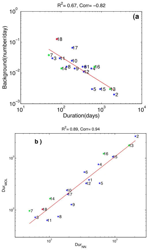
The average background daily rate is computed by using the seismicity that occurred within one year before the mainshock time and distance as 5*L around the main-shock (figure 1.7). If there is no event upto one year before the mainmain-shock then we increase the time window such as two year for average background daily rate.

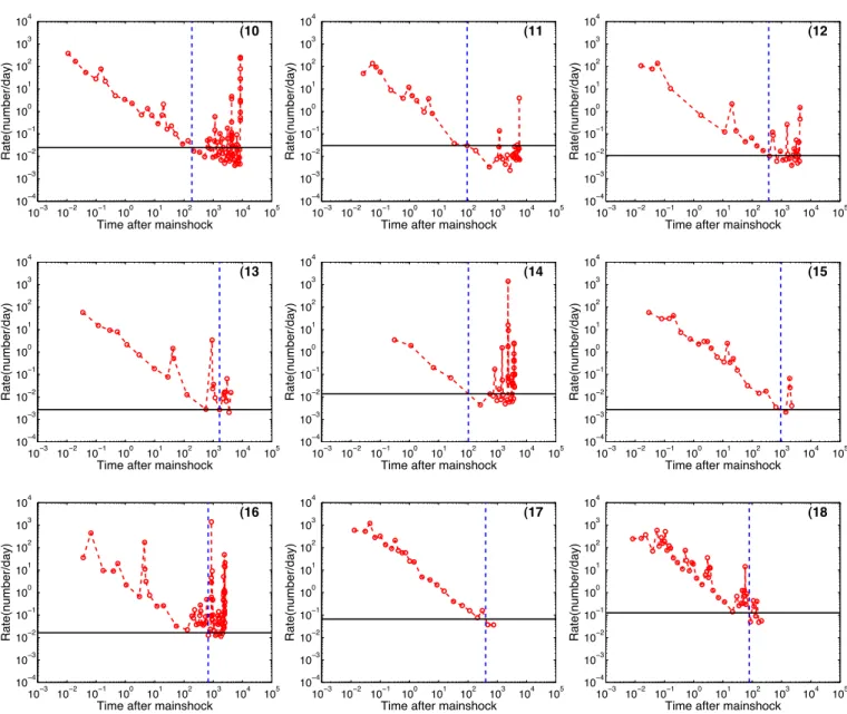
The duration of each aftershocks sequences is defined as the first return point to the background rate. Duration is estimated by using three different techniques. Firstly the duration is defined as the first return time of the weekly seismicity rate to the weekly background rate (figure 1.7c). When data sets are small, this technique give a lower bound estimate of duration, because it is sensitive to the empty bins. Secondly we compute dura-tion using nearest neighbor technique (Silverman (1986)), in which daily rate is estimated by taking inverse of the width of the box contain k neighboring points. Smoothing is con-trolled by k. The advantage of this technique is that smoothing is uniform and there are no empty bin (Felzer and Brodsky (2006)). We use k = 2, but the test was also performed for different k − values. This duration is defined as the time when the daily rate computed using nearest neighbor method (k = 2) reaches the average daily background rate (figure 1.8–1.9, table 1.2). Thirdly we calculate duration using Omori law parameters (see section

2 4 6 8 10 12 14 16 18 0 0.1 0.2 0.3 0.4 0.5 0.6 0.7 0.8 0.9 1 N Number of sequence Average +1σ Average Time=24h 2 4 6 8 10 12 14 16 18 0 0.1 0.2 0.3 0.4 0.5 0.6 0.7 0.8 0.9 1 N Number of sequence Average +1σ Average Time=48h 2 4 6 8 10 12 14 16 18 0 0.1 0.2 0.3 0.4 0.5 0.6 0.7 0.8 0.9 1 N Number of sequence Average +1σ Average Time=72h Thrust Normal Strike−Slip

(a) Aftershocks rate in 24, 48 and 72 hours after the mainshock time and for distance as 1*L arround mainshock.

2 4 6 8 10 12 14 16 18 0 0.2 0.4 0.6 0.8 1 N Number of sequence Average +1σ Average Time=24h 2 4 6 8 10 12 14 16 18 0 0.2 0.4 0.6 0.8 1 N Number of sequence Average +1σ Average Time=48h 2 4 6 8 10 12 14 16 18 0 0.2 0.4 0.6 0.8 1 N Number of sequence Average +1σ Average Time=72h

(b) Aftershocks rate in 24, 48 and 72 hours after the mainshock time and for distance as 5*L arround mainshock.

2 4 6 8 10 12 14 16 18 0 0.1 0.2 0.3 0.4 0.5 0.6 0.7 0.8 0.9 1 N Number of sequence Average +1σ Average Time=24h 2 4 6 8 10 12 14 16 18 0 0.1 0.2 0.3 0.4 0.5 0.6 0.7 0.8 0.9 1 N Number of sequence Average +1σ Average Time=48h 2 4 6 8 10 12 14 16 18 0 0.1 0.2 0.3 0.4 0.5 0.6 0.7 0.8 0.9 1 N Number of sequence Average +1σ Average Time=72h

(c) Aftershocks rate in 24, 48 and 72 hours after the mainshock time and for distance as 10*L arround mainshock.

Figure 1.5: Aftershocks rate, for time and distance window. (a) 1*L (b) 5*L (c) 10*L arround mainshock. N=(Number of aftershocks)/Nmax, Nmax=maximum number of af-tershocks.

2 4 6 8 10 12 14 16 18 0 0.1 0.2 0.3 0.4 0.5 0.6 0.7 0.8 0.9 1 N * Number of sequence Average +1σ Average Average −1σ Time=24h 2 4 6 8 10 12 14 16 18 0 0.1 0.2 0.3 0.4 0.5 0.6 0.7 0.8 0.9 1 N * Number of sequence Average +1σ Average Average −1σ Time=48h 2 4 6 8 10 12 14 16 18 0 0.1 0.2 0.3 0.4 0.5 0.6 0.7 0.8 0.9 1 N * Number of sequence Average +1σ Average Average −1σ

Time=72h ThrustNormal Strike−Slip

(a) Normalized rate of aftershocks in 24, 48 and 72 and distance as 1*L.

2 4 6 8 10 12 14 16 18 0 0.1 0.2 0.3 0.4 0.5 0.6 0.7 0.8 0.9 1 N * Number of sequence Average +1σ Average Average −1σ Time=24h 2 4 6 8 10 12 14 16 18 0 0.1 0.2 0.3 0.4 0.5 0.6 0.7 0.8 0.9 1 N * Number of sequence Average +1σ Average Average −1σ Time=48h 2 4 6 8 10 12 14 16 18 0 0.1 0.2 0.3 0.4 0.5 0.6 0.7 0.8 0.9 1 N * Number of sequence Average +1σ Average Average −1σ Time=72h

(b) Normalized rate of aftershocks in 24, 48 and 72 and distance as 5*L.

2 4 6 8 10 12 14 16 18 0 0.1 0.2 0.3 0.4 0.5 0.6 0.7 0.8 0.9 1 N * Number of sequence Average +1σ Average Average −1σ Time=24h 2 4 6 8 10 12 14 16 18 0 0.1 0.2 0.3 0.4 0.5 0.6 0.7 0.8 0.9 1 N * Number of sequence Average +1σ Average Average −1σ Time=48h 2 4 6 8 10 12 14 16 18 0 0.1 0.2 0.3 0.4 0.5 0.6 0.7 0.8 0.9 1 N * Number of sequence Average +1σ Average Average −1σ Time=72h

(c) Normalized rate of aftershocks in 24, 48 and 72 and distance as 10*L.

Figure 1.6: Normalized aftershocks rate, for time and distance window. (a) 1*L (b) 5*L

(c) 10*L. N∗ ₌ N

Nmax10mm−mc, Nmax=maximum number of aftershocks, mm is mainshock

2 4 6 8 10 12 14 16 18 0 0.1 0.2 0.3 0.4 0.5 0.6 0.7 0.8 Background(number/week) Number of sequence Average +1σ Average (a 2 4 6 8 10 12 14 16 18 0 0.02 0.04 0.06 0.08 0.1 0.12 Background(number/day) Number of sequence (b 2 4 6 8 10 12 14 16 18 0 20 40 60 80 100 Number of sequence (c Duration (day)

Figure 1.7: Background rate and duration of 18 aftershock sequences. Background rate is estimated using one year data before the mainshock, but if there is no event within this time period then we increase the time window to 2 years. (a) Background rate calculated from weekly rate. (b) Background rate calculated from daily rate. (c) Duration estimated from weekly rate.

4.3.3).

1.3.3

Omori Law Parameters

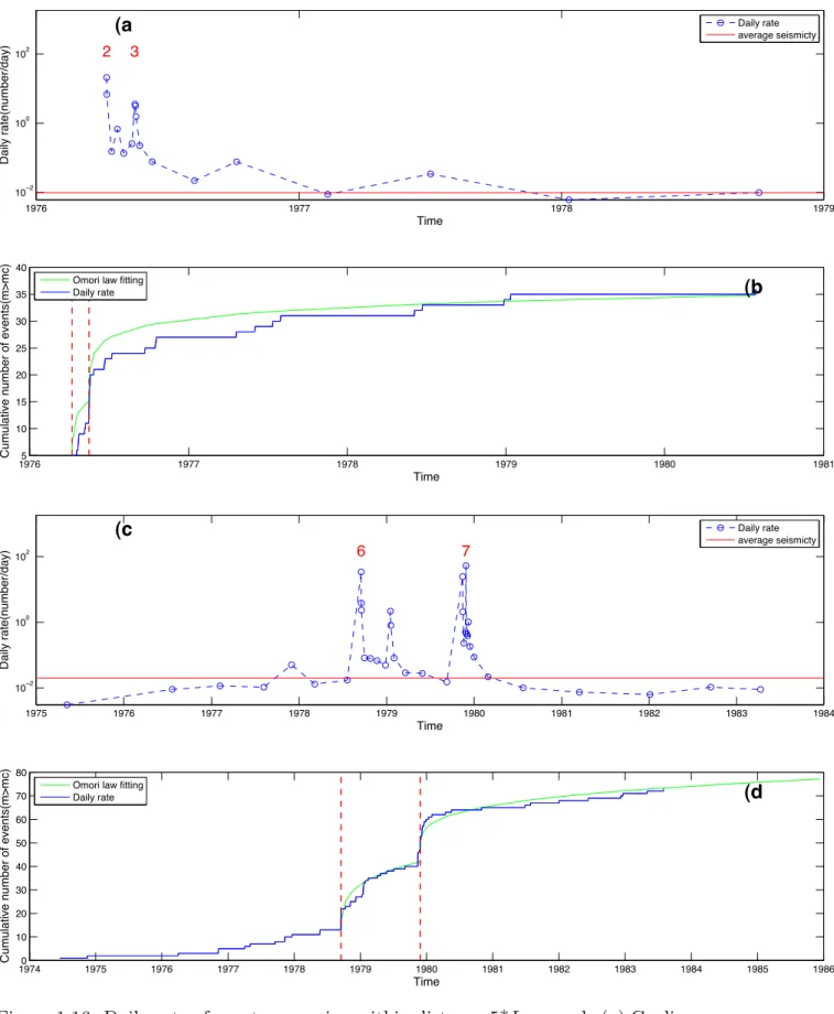
The change in time of seismicity rate following a mainshock is well reproduced by

N(t) = K

(t + c)p (1.3)

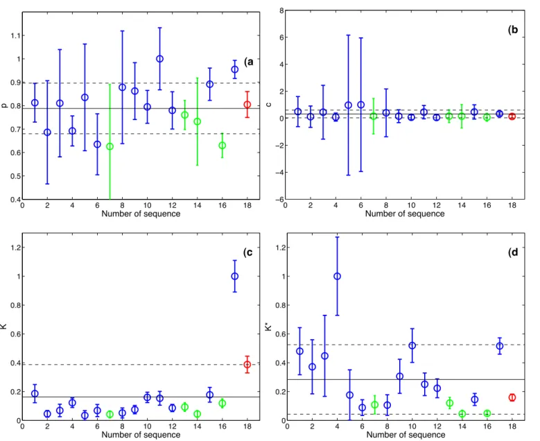
N(t) is the seismicity rate, t is the time that start from the mainshock time, p, c and K are constants (Utsu et al. (1995); Utsu (1961)). A median p − value ∼1.1 is reported for the aftershock sequences in the various parts of the world, with ∼0.6 - 2.5 range (Utsu et al. (1995)). K is the productivity of aftershocks sequences. Because K − value is a function of mainshock size, so we normalize K as;

K∗ ₌ K

10α(mm−mc) (1.4)

We used maximum likelihood method of Ogata (1983) to calculate, K, p, c, the modified Omori law parameters. The error in these parameters is strongly dependent on the number of aftershocks used to calculate these parameters (figure (1.10, 1.11)).

10−3 10−2 10−1 100 101 102 103 104 105 10−4 10−3 10−2 10−1 100 101 102 103 104

Time after mainshock

Rate(number/day) (1 10−3 10−2 10−1 100 101 102 103 104 105 10−4 10−3 10−2 10−1 100 101 102 103 104

Time after mainshock

Rate(number/day) (2 10−3 10−2 10−1 100 101 102 103 104 105 10−4 10−3 10−2 10−1 100 101 102 103 104

Time after mainshock

Rate(number/day) (3 10−3 10−2 10−1 100 101 102 103 104 105 10−4 10−3 10−2 10−1 100 101 102 103 104

Time after mainshock

Rate(number/day) (4 10−3 10−2 10−1 100 101 102 103 104 105 10−4 10−3 10−2 10−1 100 101 102 103 104

Time after mainshock

Rate(number/day) (5 10−3 10−2 10−1 100 101 102 103 104 105 10−4 10−3 10−2 10−1 100 101 102 103 104

Time after mainshock

Rate(number/day) (6 10−3 10−2 10−1 100 101 102 103 104 105 10−4 10−3 10−2 10−1 100 101 102 103 104

Time after mainshock

Rate(number/day) (7 10−3 10−2 10−1 100 101 102 103 104 105 10−4 10−3 10−2 10−1 100 101 102 103 104

Time after mainshock

Rate(number/day) (8 10−3 10−2 10−1 100 101 102 103 104 105 10−4 10−3 10−2 10−1 100 101 102 103 104

Time after mainshock

Rate(number/day)

10−3 10−2 10−1 100 101 102 103 104 105 10−4 10−3 10−2 10−1 100 101 102 103 104

Time after mainshock

Rate(number/day) (10 10−3 10−2 10−1 100 101 102 103 104 105 10−4 10−3 10−2 10−1 100 101 102 103 104

Time after mainshock

Rate(number/day) (11 10−3 10−2 10−1 100 101 102 103 104 105 10−4 10−3 10−2 10−1 100 101 102 103 104

Time after mainshock

Rate(number/day) (12 10−3 10−2 10−1 100 101 102 103 104 105 10−4 10−3 10−2 10−1 100 101 102 103 104

Time after mainshock

Rate(number/day) (13 10−3 10−2 10−1 100 101 102 103 104 105 10−4 10−3 10−2 10−1 100 101 102 103 104

Time after mainshock

Rate(number/day) (14 10−3 10−2 10−1 100 101 102 103 104 105 10−4 10−3 10−2 10−1 100 101 102 103 104

Time after mainshock

Rate(number/day) (15 10−3 10−2 10−1 100 101 102 103 104 105 10−4 10−3 10−2 10−1 100 101 102 103 104

Time after mainshock

Rate(number/day) (16 10−3 10−2 10−1 100 101 102 103 104 105 10−4 10−3 10−2 10−1 100 101 102 103 104

Time after mainshock

Rate(number/day) (17 10−3 10−2 10−1 100 101 102 103 104 105 10−4 10−3 10−2 10−1 100 101 102 103 104

Time after mainshock

Rate(number/day)

(18

Figure 1.8: Duration of aftershock sequences estimated by using nearest neighbour method. Aftershocks are taken within distance = 5*L around mainshock. Blue dotted line shows the position where daily rate (red) first time goes to average daily background rate (black). Average background rate is calculated using events 1yr, 5L around the mainshock.

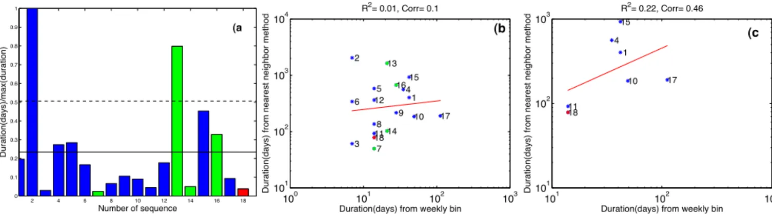
2 4 6 8 10 12 14 16 18 0 0.1 0.2 0.3 0.4 0.5 0.6 0.7 0.8 0.9 1 Duration(days)/max(duration) Number of sequence (a 100 101 102 103 101 102 103 104 1 2 3 4 5 6 7 8 9 ₁₀ 11 12 13 14 15 16 17 18 R2= 0.01, Corr= 0.1

Duration(days) from weekly bin

Duration(days) from nearest neighbor method

(b 101 102 103 101 102 103 1 4 10 11 15 17 18 R2= 0.22, Corr= 0.46

Duration(days) from weekly bin

Duration(days) from nearest neighbor method

(c

Figure 1.9: Duration (days) estimated from daily rate. (a) Duration estimated by using nearest neighbor method with smoothing factor k = 2, k is the number of points taken inside the bin used to calculate the rate, higher k the more will be smooth the data, but for small data higher k cannot be used. (b) Comparison between the duration calculated from nearest neighbor method and weekly bin method. (c) The same comparison as in (a), but in this case we have only those sequences with number of aftershock greater then 20.

Using Omori law parameters we estimate duration as the time when the rate reaches the background rate (figure (1.10, 1.12a)). Then we compare these duration estimates with that deduced from nearest neighbor method (figure 1.12b).

1.3.4

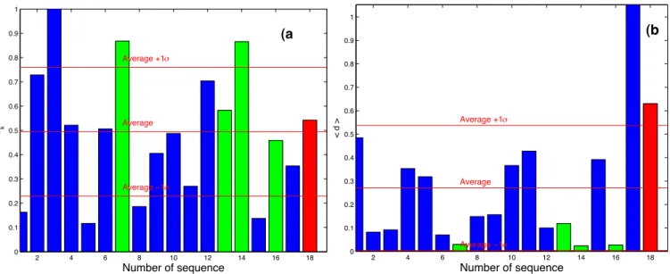
Size of Aftershock zone and average aftershock density

Following Kagan (2002a) we estimated the size of the aftershock zone as;

Sk = 4σj (1.5) σj = ! 1 2(N − 1)(xx + yy +"(xx − yy) 2_{+ 4ρ}2 a∗ xx ∗ yy) (1.6) σn = ! 1 2(N − 1)(xx + yy −"(xx − yy) 2_{+ 4ρ}2 a∗ xx ∗ yy) (1.7) whereas ρa = _√xx∗yyxy