TH `ESE
TH `ESE
En vue de l’obtention du
DOCTORAT DE L’UNIVERSIT´
E DE TOULOUSE
D´elivr´e par : l’Universit´e Toulouse 3 Paul Sabatier (UT3 Paul Sabatier)
Pr´esent´ee et soutenue le 12/10/2018 par :
Margaux HOANG ´
Etude de la coma de la com`ete 67P/Churyumov-Gerasimenko `a l’aide des donn´ees de l’instrument ROSINA/RTOF à bord de la mission
spatiale Rosetta.
JURY
Henri REME Professeur émérite Pr´esident du Jury
Philippe GARNIER Maître de conférence Membre du Jury
J´er´emie LASUE Astronome adjoint Membre du Jury
Dominique
BOCKELEE-MORVAN
Directrice de recherche Membre du Jury
Val´erie CIARLETTI Professeure Membre du Jury
Nicolas BIVER Chargé de recherche Membre du Jury
Anny-Chantal
LEVASSEUR-REGOURD
Professeure émérite Membre du Jury
´
Ecole doctorale et sp´ecialit´e :
SDU2E : Astrophysique, Sciences de l’Espace, Plan´etologie
Unit´e de Recherche :
Institut de Recherche en Astrophysique et Plan´etologie (UMR 5277)
Directeur(s) de Th`ese :
Philippe GARNIER et J´er´emie LASUE
Rapporteurs :
i
Le travail présenté dans cette thèse a été réalisé à l’Institut de Recherche en Astro-physique et Planétologie de Toulouse, et encadré par Philippe Garnier et Jérémie Lasue, mes directeurs de thèse, que je remercie ici sincèrement. Je remercie également Henri, Dominique, Arnaud, ainsi que Benoˆıt, Josette, Dorine, Henda et toutes les personnes du laboratoire qui m’ont aidée et soutenue durant ces trois ans.
Je remercie l’équipe ROSINA du Center for Space and Habitability de l’Université de Bern, en particulier Sébastien Gasc, Kathrin Altwegg et Martin Rubin. Je remercie également Maria Teresa Capria de l’Istituto Naziolane di Astrofisica de Rome.
Je remercie Dominique Bockelée-Morvan et Valérie Ciarletti d’avoir accepté d’être rapportrices de ma thèse, ainsi que Nicolas Biver et Anny-Chantal Levasseur-Regourd d’avoir fait partie de mon jury.
Enfin, cette aventure m’a permise de rencontrer une pléiade de personnes exception-nelles: Merci à Cricri, Gab, Jason, Marina, Zizi, Sinon, Sacha, Mathieu, Ilane, Victor, Tonio, Henda, Sophie, Rémi, Jacqueline et Gilbert.
iii
Far above the world Planet Earth is blue And there’s nothing I can do
Contents
Abstract xvii
R´esum´e xix
General introduction xxi
Introduction g´en´erale xxiii
I
Comets: small icy bodies of the Solar System
1
1 From naked-eye observation to in situ. 3
1.1 Observations through the ages . . . 3
1.2 Origin of comets and their importance . . . 5
1.3 Interest of the cometary science . . . 8
1.4 Comet types and classification . . . 8
1.5 Structure . . . 9
1.5.1 Nucleus . . . 9
1.5.2 Coma . . . 10
1.5.3 Tails . . . 10
1.6 Observations before Rosetta . . . 11
2 Our vision of the coma and the nucleus 17 2.1 Coma . . . 17
2.1.1 Chemical composition of the coma . . . 17
2.1.2 Photo-reactions and chemical reactions . . . 19
2.1.3 Models of gas expansion in the coma . . . 20
2.2 Cometary nucleus . . . 22
2.2.1 Model of the internal structure . . . 22
2.2.2 Heat diffusion and physical processes . . . 25
3 The Rosetta mission (2014-2016) 29 3.1 Introduction . . . 29
3.2 Comet 67P/Churyumov-Gerasimenko . . . 30
3.3 On-board instruments . . . 30
3.4 Trajectory . . . 32
3.5 Overview of the main scientific results . . . 35
II
Description of the experiment and data analysis
43
4 The ROSINA experiment 45
4.1 General presentation . . . 45
4.2 Science objectives and performance . . . 46
4.3 Mass spectrometry . . . 46
4.3.1 Time-of-flight mass spectrometry . . . 48
4.4 Description of the ROSINA instruments . . . 50
4.4.1 The Double Focusing Mass Spectrometer . . . 50
4.4.2 The COmet Pressure Sensor . . . 51
4.5 The Reflectron-type Time-Of-Flight mass spectrometer . . . 51
4.5.1 Instrument description . . . 52
4.5.2 Principle . . . 55
4.5.3 Operating modes . . . 55
4.5.4 In flight performance limitations . . . 56
5 Data analysis of RTOF spectra 57 5.1 RTOF raw spectra . . . 58
5.1.1 Acquisition . . . 58
5.1.2 ADC Correction . . . 58
5.1.3 Baseline . . . 58
5.1.4 Electronic noise and other non desirable peaks . . . 59
5.2 RTOF L3 spectra . . . 59
5.2.1 Mass calibration . . . 59
5.2.2 Abundance of volatiles . . . 62
5.3 Conversion to volatiles density . . . 62
5.3.1 Fragmentation . . . 63
5.3.2 Sensitivity . . . 64
5.3.3 COPS calibration . . . 65
III
The heterogeneous coma of 67P/C-G seen by ROSINA 67
6 Description of the datasets 71 6.1 Orbitography parameters . . . 716.1.1 Sub-spacecraft point coordinates . . . 71
6.1.2 67P/C-G’s orbit . . . 71
6.1.3 Spacecraft to comet distance . . . 74
6.1.4 Nadir off-pointing . . . 75
6.2 RTOF dataset . . . 75
7 Global dynamics of the main volatiles 77 7.1 Dependence on the comet-spacecraft distance . . . 77
7.2 Diurnal variation . . . 78
7.3 Evolution of the activity with the heliocentric distance . . . 81
7.3.1 Global pattern . . . 81
CONTENTS vii 7.4 Seasonal variations . . . 84 7.4.1 Approach . . . 86 7.4.2 Pre-equinox 1 . . . 86 7.4.3 Pre-equinox 2 . . . 87 7.4.4 Post-equinox 2 . . . 88 7.4.5 End of mission . . . 88
7.5 Evolution of density ratios . . . 90
8 Spatial variation of the main volatiles 93 8.1 The geographical coordinate system . . . 93
8.2 Illumination model . . . 94
8.3 Density maps through the mission . . . 96
8.3.1 Description of the maps . . . 96
8.3.2 Analysis of the density maps . . . 99
8.3.3 Interpretation of the observations . . . 100
8.3.4 Difference between the two lobes . . . 102
8.4 Detection of molecular oxygen . . . 104
8.4.1 Method . . . 105
8.4.2 Analysis . . . 107
9 Comparison with DFMS 109 9.1 Cross correlation RTOF vs DFMS . . . 109
9.2 DFMS density maps . . . 112
10 Comparison with a numerical model of the coma 117 10.1 DSMC model . . . 117
10.2 Comparison with RTOF density . . . 118
10.3 Global comparison between ROSINA and the DSMC model . . . 121
IV
Simulating the nucleus to constrain properties
125
11 The thermo-physical model 127 11.1 Description of the model . . . 12711.1.1 Description of the algorithm . . . 130
11.2 Previous studies . . . 130
11.3 Application of the model . . . 130
11.3.1 Orbital parameters . . . 130
11.3.2 Physical parameters . . . 131
11.3.3 Computed locations and description of the cases . . . 132
12 Analysis of the nucleus model results 135 12.1 Evolution of the surface and interior’s temperature . . . 135
12.2 Evolution of the stratification . . . 138
12.3 Evolution of the fluxes . . . 140
12.4 Effect of the dust layer and of the trapping conditions . . . 142
12.4.2 Effect of the trapped CO on the averaged fluxes . . . 143
12.5 Analysis of the production rate . . . 145
13 Comparison with fluxes derived from RTOF 149 13.1 Global comparison with RTOF . . . 149
13.1.1 Deriving surface production rates from RTOF . . . 149
13.1.2 Comparison with RTOF global production rates . . . 150
13.2 Comparison of the flux geographical maps . . . 151
13.2.1 Visualisation and Interpolation . . . 151
13.2.2 Analysis of the model maps . . . 151
13.2.3 Comparison with the RTOF spatial variation . . . 156
13.3 Discussion and perspectives . . . 158
Conclusion and perspectives (English version) 161 Conclusion et perspectives (french version) 165
List of Figures
1.1 Representation of the Halley’s comet passage of 1066 in a part of the Bayeux embroideries where the text says: Isti mirant stella, Those men wonder at the star (1070) (Archeurope Educational Resources, 2018). . . 4 1.2 Representation of the planetary migration and their effect on the small
bodies of the Solar System, as described by the Grand Tack and the Nice model (DeMeo and Carry, 2014). . . 6 1.3 Schematic of the Solar System, showing the Main Asteroid Belt (between
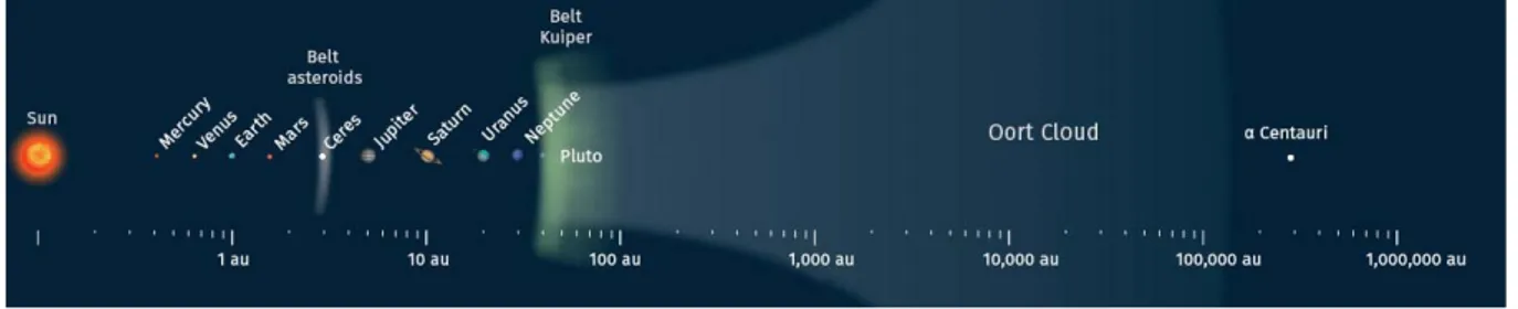
the orbits of Mars and Jupiter), the Kuiper belt (from 30 to 50 AU from the Sun) and the Oort cloud (up to 50 000-100 000 AU). Modified from an illustration from Schwamb (2014). . . 7 1.4 Structure of a comet, annotated on a picture of 1P/Halley taken in 1986
(Credits: W: Liller). Cometary tails are the only visible part of the comet from Earth. . . 10 1.5 Top left: The 21 fragments of the disrupted D/1993 F2 (Shoemaker-Levy
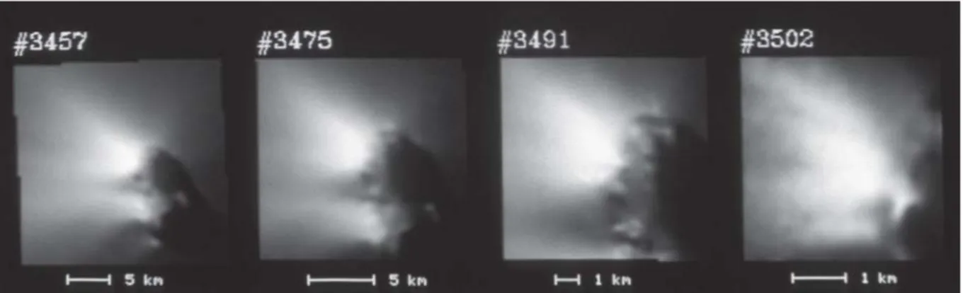
9), taken on the 17 May 1994. NASA/ESA. Top right: Dark patches on the southern hemisphere of Jupiter’s atmosphere, following the impact of the fragments, pictured by the Hubble Space Telescope in July 1994. Bottom: Trail of debris of the disrupted comet 73P/Schwassmann-Wachmann 3, pictured by the Spitzer Space Telescope in May 2006. . . 14 1.6 Six pictures of comet 1P/Halley taken by the Halley Multicolour Camera
(HCM) in March 1986. . . 15 1.7 Nuclei of the visited (and pictured) comets 1P/Halley, 81P/Wild 2, 16P/Borrelly,
9P/Tempel 1, 103P/Hartley 2. Montage based on a work from Emily Lak-dawalla. Picture credits: Russian Academy of Sciences (Halley), NASA/JPL (Borelly, Tempel 1, Hartley 2 and Wild 2). . . 15
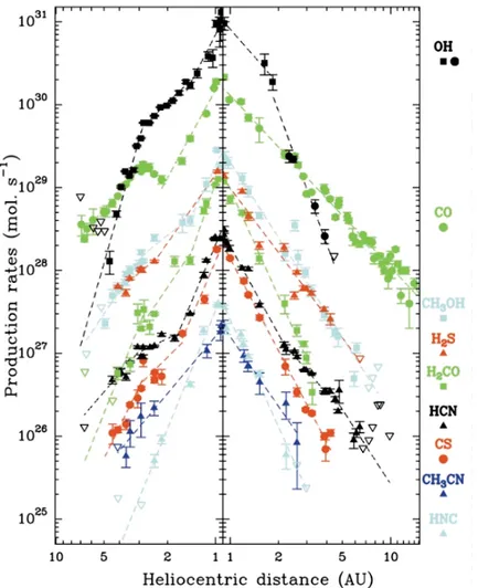
2.1 Production rate of volatiles with respect to the heliocentric distance of comet C/1995 O1 (Hale-Bopp) (Biver et al., 2002). . . 18 2.2 Observation of the O I line from water (short-dashed curve) and from OH
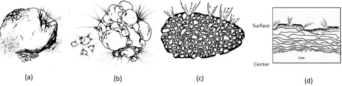
(long-dashed curve) observed in comet 1P/Halley and the curve obtained with the Haser model (solid curve) (Magee-Sauer et al., 1988). . . 22 2.3 Representations of four models of cometary nucleus: (a) the icy
conglom-erate model (Whipple, 1950), (b) the rubble pile model (Weissman, 1986), (c) the icy-glue model (Gombosi and Houpis, 1986) and (d) the layered pile model (Belton et al., 2007). Credits: unknown. . . 25
2.4 Effect of the solar illumination on an hypothetical nucleus model containing amorphous ice, and example of induced stratification, based on Prialnik (2004). The heat wave propagation leads to an erosion of the surface, gas and dust ejection with eventual release of minor species, the formation of a dust mantle and a stratification of the nucleus’ interior. The colored points represented eventual volatiles species trapped in the amorphous ice. The depth of the layers are not scaled, the heating decreases exponentially with the depth, therefore the layers are closer to each other near the surface, the pristine material being located at an unknown depth. . . 27 3.1 Schematics of the Rosetta orbiter, with the location of the 11 instruments
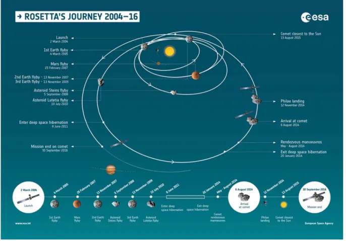
(upper figure) and the lander Philae, with the location of its 10 instruments (lower figure) (Balsiger et al., 2007). . . 33 3.2 Rosetta’s trajectory from Earth to 67P/C-G, with fly-bys of the Earth,
Mars, the asteroid Stein and Lutetia. Credit: NASA/ESA. . . 34 3.3 Left: View at 100 km from the surface of asteroid (21) Lutetia with, in the
background, Saturn. Right: view at 800 km from asteroid (2867) ˇSteins. Pictured by OSIRIS. Credits: ESA/Rosetta/MPS for OSIRIS Team. . . 35 3.4 Left: Picture taken by OSIRIS on the 2 September 2016 at 2.7 km from
the surface, which allowed to identify Philae less than month before the end of the mission. The image scale is 5 cm/pixels and Philae’s size is „ 1 m. Would the reader be able to find Philae? Ñ Find the solution at the end of the document. Right: The location of Philae on the nucleus and a zoom on the lander wedged into a crack. . . 36 3.5 Last picture of the Rosetta mission, taken by OSIRIS from an altitude of
24.7 ˘ 1.5 m. Credit: ESA/Rosetta/MPS for OSIRIS Team. . . 36 3.6 Pictures of the bilobate comet 67P{Churyumov-Gerasimenko taken
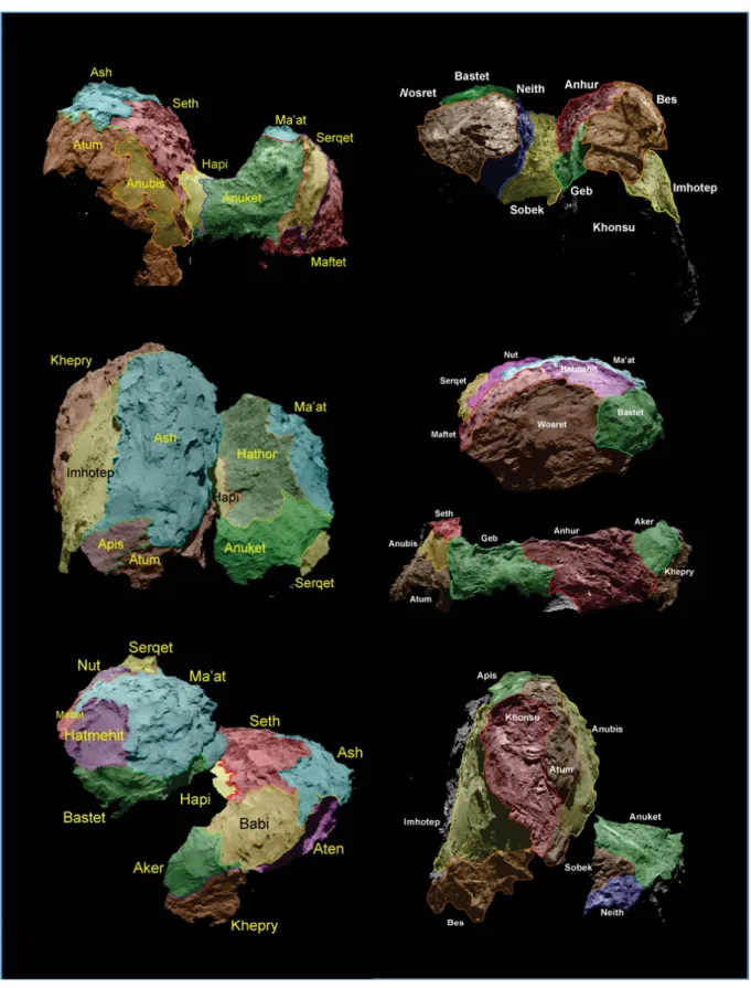
dur-ing the Rosetta mission, on the 3rd August 2014 (upper picture) and 28 January 2016 (lower picture). Credits: ESA/Rosetta/MPS and /NAVCAM. 38 3.7 The regions boundaries and names of 67P/C-G’s northern hemisphere (left
side) and southern hemisphere (right side). Credits: ESA/Rosetta/MPS for OSIRIS Team. . . 39 3.8 The ROSINA zoo illustrates the diversity of the molecules detected in the
coma of 67P/C-G by ROSINA/DFMS. Credits: ESA. . . 41 4.1 Sketch of a linear Time-Of-Flight mass spectrometer. The atoms and
molecules are first ionised. All ions receive the same kinetic energy. They are separated by their masses in the acceleration region, sent in a field free drift region before they finally reach a detector. The lighter ions (with the smaller mass/ratio) travel faster and are the first detected. Lower figure: a corresponding typical TOF spectrum, in abundance versus time-of-flight. The resolution decreases with the mass, leading to broader peaks for the heavier masses. . . 48 4.2 Sketch of the time spread due to spatial distribution (a) and kinetic energy
distribution (b). The ions with same m/q have slightly different speeds and the mass resolution decreases, leading to a broadening (and eventually overlap) of the peaks (c). . . 49
LIST OF FIGURES xi
4.3 Sketch of a Time-Of-Flight mass spectrometer equipped with a reflectron. The introduction of a reflectron compensates for the spatial and kinetic energy distributions by synchronising the ions in time, which increases the mass resolution. . . 50 4.4 Picture of ROSINA/DFMS (left), an instrument of 63ˆ 63 ˆ 26 cm for a
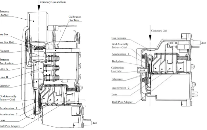
mass of 16.2 kg. Picture of ROSINA/COPS (right), an instrument of 26ˆ 26ˆ 17 cm for a mass of 1.6. Credits: University of Bern. . . 52 4.5 Picture of ROSINA/RTOF, an instrument of 114ˆ 38 ˆ 24 cm for a mass
of 14.7 kg. Credits: University of Bern. . . 53 4.6 Schematic of the RTOF mass spectrometer (Balsiger et al., 2007). . . 53 4.7 Schematics of the two RTOF’s ion sources: Orthogonal Source (left) and
Storage Source (right). From Balsiger et al. (2007). . . 54 4.8 Sketch of simple-reflection mode (a) and triple reflection modes (b). The
elongation of the path induced by the triple reflection modes increases the mass resolution. . . 55 5.1 Schematic of the data analysis: L2 are the raw RTOF spectra, L3 are
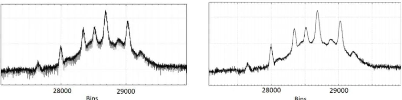
the mass calibrated spectra and L5 are the temporal evolutions for species density (note that there are no L4 spectra for RTOF). . . 57 5.2 Denoising of the ADC pattern. Zoom on a SS spectrum before (left) and
after (right) ADC correction. . . 59 5.3 Electronic peaks (indicated with red crosses) in a SS spectrum. Credits: S.
Gasc. . . 60 5.4 Mass scale of a level 2 GCU spectrum (upper figure) to a level 3 spectrum
(lower figure) and electronic peaks correction. . . 61 5.5 Zoom of a L3 RTOF spectra: peaks of H2O, CO and CO2 with the
pseudo-Voigt function’s fitting in red. The fitting appeared to be a non-convincing method of quantification, and was substituted by a numerical integration. 62 5.6 Main interfaces of the RTOF spectra analyser software (version 8.5),
de-veloped by S. Gasc and tested in Toulouse. . . 63 6.1 Four top panels: Sub-spacecraft latitude (orange lines) and longitude (white
lines). Bottom: 2D map representation of the comet 67P/C-G. . . 72 6.2 Left panel: orbit of 67P/C-G (in blue), with the rendez-vous with Rosetta
in August 2014 (1), the first equinox on 10 May 2015 (2), perihelion on 13 August 2015 (3) and the second equinox on 21 March 2016 (4). The Earth’s orbit is shown in green. Right: Shape of 67P/C-G with its equatorial axis (x axis in red and y axis in green) and its rotation axis (in blue), tilted by 52˝. The orbit of 67P/C-G has an inclination of 7˝ with respect to the ecliptic plane. Credits: ESA/Rosetta/MPS for OSIRIS Team. . . 73 6.3 Upper panel: heliocentric distance. Lower panel: latitude of the position
of the Sun in the comet fixed frame. . . 73 6.4 Variation of the distance between the spacecraft and the comet during the
mission (upper panel), zoom on the closer distances (middle panel), and variation of the phase angle (lower panel). . . 74 6.5 SS neutrals (blue), OS neutrals (green) and OS ions (red) operation modes
7.1 Dependence between the COPS pressure and the altitude of the spacecraft after the 14th February 2015’s fly-by. . . 78 7.2 Diurnal variation of main volatiles. Upper panel: densities of H2O, CO
and CO2 from 8 October to 11 October 2014. Middle panel: sub-spacecraft point longitude and latitude variations during the same period. Low panel: views of the comet from the spacecraft at specific times marked as 1, 2, 3 and 4 on the upper panel. Figure modified from Hoang et al. (2017). . . . 79 7.3 Lomb-scargle periodogram of H2O (left), with strong periodicities at 6 and
12 hours, and of CO2 (right), with a more homogeneous behaviour and a main periodicity of 12 hours. . . 80 7.4 Total density from COPS, as well as the H2O, CO2, and CO densities from
RTOF during the approach as a function of the local time. Densities were normalised at a constant 10 km altitude. . . 81 7.5 Upper panel: temporal evolution of H2O, CO2 and CO densities corrected
for distance effect, seen by the RTOF spectrometer over the Rosetta mis-sion. Coloured lines are averaged over two comet rotations. Middle panel: latitude of the sub-spacecraft point in the 67P/C-G fixed frame. Lower panel: variation of the heliocentric distance (red) and the distance between Rosetta and 67P/C-G (blue). RTOF data are missing during excursions of the spacecraft. First equinox occurred on 2015/05/10 at 1.67 AU, perihe-lion on 2015/08/13 at 1.24 AU, and second equinox on 2016/03/21 at 2.63 AU. From Hoang et al., 2018 (to be submitted). . . 82 7.6 Outgassing rate from COPS and prediction of activity from Snodgrass et al.
(2013). . . 83 7.7 Water production rate as a function of the heliocentric distance (Hansen
et al., 2016), from different instruments onboard Rosetta (ROSINA, VIR-TIS, RPC-ICA and MIRO), as well as the estimated dust production rate. The maximum of water outgassing occured 18 - 22 days after perihelion. . 84 7.8 Illustration of 67P/C-G and Earth’s orbits with the position of the comet
at the equinoxes and perihelion, and during the five periods described in Table 7.1. . . 85 7.9 Densities of the main volatiles during the approach time period. . . 86 7.10 Densities of the main volatiles during the pre-equinox 1 time period. . . . 87 7.11 Densities of the main volatiles during the pre-equinox 2 time period . . . . 88 7.12 Densities of the main volatiles during the post-equinox 2 time period. . . 89 7.13 Densities of the main volatiles (zoom on the last days of the mission). . . 90 7.14 Upper panel: time evolution of CO/H2O and CO2/H2O average density
ratios for the entire mission, starting in September 2014 and ending in September 2016. Lower panel: variation of the sub-spacecraft point’s lati-tude in degrees. . . 91 7.15 CO2/H2O density ratio from RTOF as a function of H2O density from 24
November 2014 to 24 January 2015 (left). This figure is compared with the similar analysis in Fig. 11 published in Bockel´ee-Morvan et al. (2015) (right), where the colors indicated the observed regions. . . 91
LIST OF FIGURES xiii
8.1 Two-dimensional longitude/latitude representation of the morphological re-gions of 67P/C-G as defined in El-Maarry et al. (2015). Credit: OSIRIS Team. . . 94 8.2 Left: variation of the heliocentric distance and sub-solar point latitude for
the five studied periods. Right: 2D longitude/latitude maps of average illumination during the five periods. . . 95 8.3 Spatial heterogeneities of the coma for the approach (top) and pre-equinox
1 time period (bottom), for H2O (left), CO2(middle) and CO (right) densities. 97 8.4 Spatial heterogeneities of the coma for pre-equinox 2 (top), post-equinox
2 (middle) and end of mission (bottom) time period, for H2O (left), CO2 (middle) and CO (right) densities. . . 98 8.5 Time evolution of CO/H2O and CO2/H2O density ratios for the entire
mission for the northern hemisphere (upper panel) and the southern hemi-sphere (lower panel). . . 102 8.6 Study of the difference between the two lobes. CO2/H2O (top) and CO/H2O
(bottom) as a function of H2O density (top) for the big lobe and the small lobe. . . 103 8.7 DFMS spectra acquired at 5 different time periods, showing the most
abun-dant species detected at mass 32 over the mission (Bieler et al., 2015). . . . 105 8.8 Abundances of O2 (blue), CH3OH (yellow) and S (orange) detected by
DFMS through the whole mission. . . 106 8.9 Sensitivities versus ionization cross section [ˆ 10´16] cm2 for RTOF SS and
OS modes (Gasc et al., 2017b). . . 107 8.10 Temporal evolution of H2O (blue) and O2 (orange, with a moving average
in yellow) densities from RTOF (upper panel) and DFMS (lower panel) over the approach period. . . 108 8.11 Map of O2 density in molecules/cm3 averaged over the approach time period.108 9.1 Cross correlation between RTOF and DFMS for H2O (upper panel), CO2
(middle panel) and CO (lower panel). . . 110 9.2 Correlation factor between the DFMS and RTOF measurements, for H2O
(upper panel), CO2 (middle panel) and CO (lower panel). . . 110 9.3 Temporal evolution of the main volatiles’s densities after outbound equinox
(first panel), DFMS corresponding densities (second panel), COPS nude gauge total densities (third panel) and sub-spacecraft point latitude and longitude (fourth panel). . . 111 9.4 CO2/H2O (upper panel) and CO/H2O (middle panel) ratios from RTOF
and DFMS during pre-equinox 1, with the variation of the SSC latitude (lower panel). . . 112 9.5 Spatial heterogeneities of the coma for the approach (top) and pre-equinox
1 (bottom) time periods, for H2O (left), CO2 (middle) and CO (right) densities, measured by DFMS. . . 113 9.6 Spatial heterogeneities of the coma for pre-equinox 2 (top), post-equinox
2 (middle) and end of mission (bottom) time periods, for H2O (left), CO2 (middle) and CO (right) densities, measured by DFMS. . . 114
9.7 Two-dimensional maps of CO2/H2O (upper panels) and CO/H2O (lower panels) density ratios based on RTOF (left) and DFMS (right) data for the pre-equinox 1 period. . . 115
10.1 2D maps of the H2O (top left) and CO2 (bottom left) modeled activity distribution at the surface of the nucleus described with a 25-term spher-ical harmonic expansion. Simulation of density (n) and streamlines for 23 December 2014 at 12:00:00 UT (Fougere et al., 2016) (right). . . 118 10.2 Density measured by DFMS (H2O in blue and CO2 in orange) and the
DSMC density extracted at the location of spacecraft (in black) (Fougere et al., 2016). . . 119 10.3 Diurnal variations of the H2O and CO2 densities: comparison between
RTOF measurements and the results from the DSMC model. . . 120 10.4 Comparison between the in situ data from RTOF and the data from the
DSMC model for H2O (upper panel) and CO2(middle panel). Lower panel: sub-spacecraft (SSC) longitude and latitude. . . 120 10.5 DSMC/RTOF ratio for H2O and CO2 for the approach (upper panel) and
pre-equinox 1 (lower panel), with their corresponding sliding average (solid lines). . . 121 10.6 Temporal evolution of H2O and CO2 densities measured by RTOF (upper
panel) and DFMS (second panel) during pre-equinox 1. Third panel: COPS nude gauge total densities. Fourth panel: H2O and CO2 densities derived from the DSMC model. Lower panel: phase-angle variations in blue and nadir off-pointing angle variations in green. From Hoang et al. (2017). . . . 123
11.1 Schematic of a porous dust layer, with the three paths of heat transport represented by arrows, from Gundlach and Blum (2012). The layer is composed of dust aggregates made of micrometer-sized particle aggregates. 129 11.2 Northern view, with the neck (left), equatorial view (middle) and southern
view (right) of the water erosion averaged over one orbit (Keller et al., 2015b). The erosion is drastically different between the northern and the southern hemisphere, indeed the northern hemisphere experienced a long and soft summer while the southern hemisphere is strongly heated by the solar illumination at close distance to the Sun. . . 132 11.3 2D latitude-longitude map of 67P/C-G with the regions (El-Maarry et al.,
2015) and the position of the 24 points studied in this work. . . 133
12.1 Evolution of the temperature of the different depths for nine chosen loca-tions, over two rotations at a heliocentric distance of 3.4 AU. The locations in the northern hemisphere (first line) are computed with the case dust 0 and the locations at the equator (second line) and in the southern hemi-sphere (third line) with the case ice 0. Layer 0 represents the surface, layer 1 is at a depth of 1 cm, layer 5 is at 5 cm, layer 10 is at 10 cm and layer 20 is at 20 cm. . . 136 12.2 Evolution of the temperature of the different depths for nine chosen
LIST OF FIGURES xv
12.3 Three typical patterns of evolution of the temperature (top) with their specific illumination conditions (bottom). Shadowing is indicated by blue arrows. The point 18 at 3.4 AU (left panel) is located in the big lobe, it experience clear day and night illumination, without self-shadowing, the point 16 at 1.9 AU (middle panel) is located between the neck and the small lobe, it experienced a shadowing due the concavity of the neck, and the point 2 at 1.9 AU (right panel) is on the southern part of the small lobe, and is very few illuminated.) . . . 138 12.4 Evolution of the stratification for three locations: in the northern
hemi-sphere (left), at the equator (middle) and in the southern hemihemi-sphere (right). The second and the third lines are zooms of the first line. . . 139 12.5 Evolution of the H2O, CO2 and CO outgassing for the point 15 of latitude
30 and longitude 75 during 5 days at 3.4 AU (upper panel) and 5 days at 2.3 AU (lower panel) in case dust 1. . . 140 12.6 Temperatures at different depths for the point of latitude 30 and longitude
75 during 5 days at 3.4 AU (upper panel) and 5 days at 2.3 AU (lower panel) in case dust 1. . . 141 12.7 Effect of the initial dust layer on the stratification of the location 15
(lat-itude 30 and lat(lat-itude 45). Left: case dust 2 (initial dust layer of 0.07 m). Middle: case dust 1b (0.1 m). Right: case dust 1a (0.2 m). . . 143 12.8 Evolution of fluxes from the point 15 (lat 30, lon 45), for H2O (top), CO2
(middle) and CO (bottom), in case dust 1 (initial dust layer of 0 m of thickness), case dust 2 (0.07 m), case dust 1b (0.1 m) and case dust 1a (0.2 m), from about 3.45 AU to 2.3 AU. . . 144 12.9 Evolution of fluxes from the point 15 (lat 30, lon 45), for H2O (top), CO2
(middle) and CO (bottom), in case dust 1b (no trapped CO) and case dust 1c (presence of trapped CO), from about 3.45 AU to 2.3 AU. . . 145 12.10Comet gas production rate [s´1] with the set of parameters dust 0 - ice 0
(top panel), dust 1 - ice 1 (second panel) and dust 2 - ice 2 (third panel) from about 3.45 AU to 2.3 AU. . . 147
13.1 Example of interpolation using the Green’s functions for splines in tension. Map of 24 studied locations (top left), 2D visualisation (top right), where the white facets are due to the non-convex shape of the nucleus, and pro-jected on 3D shape (four bottom’s figures) visualisation after interpolation over all the surface regions. In this example, colours represent the surface temperature of the nucleus around 3.3 au. . . 152 13.2 3D and 2D representations of the H2O averaged fluxes [s´1] for the approach
(six left panels) and the pre-equinox 1 (six right panels) periods with the three computations: dust 0 - ice 0 (first line), dust 1 - ice 1 (second line) and dust 2 - ice 2 (third line). The dust 0, dust 1 and dust 2 sets of parameters are used to computed the northern points and the ice 0, ice 1 and ice 2 sets of parameters are used for the equator and southern points. . 153
13.3 3D and 2D representations of the CO2averaged fluxes [s´1] for the approach (six left panels) and the pre-equinox 1 (six right panels) periods with the three computations: dust 0 - ice 0 (first line), dust 1 - ice 1 (second line) and dust 2 - ice 2 (third line). The dust 0, dust 1 and dust 2 sets of parameters are used to computed the northern points and the ice 0, ice 1 and ice 2 sets of parameters are used for the equator and southern points. . 154 13.4 3D and 2D representations of the CO averaged fluxes [s´1] for the approach
(six left panels) and the pre-equinox 1 (six right panels) periods with the three computations: dust 0 - ice 0 (first line), dust 1 - ice 1 (second line) and dust 2 - ice 2 (third line). The dust 0, dust 1 and dust 2 sets of parameters are used to computed the northern points and the ice 0, ice 1 and ice2 sets of parameters are used for the equator and southern points. . 155 13.5 Map of the difference of average surface temperature between the approach
and the pre-equinox 1 periods. . . 156 13.6 RTOF mean fluxes [s´1] for the approach (left) and pre-equinox 1 (right)
Abstract
The comet 67P/Churyumov-Gerasimenko (67P/C-G) has been investigated by the Rosetta space mission over two years from August 2014 to September 2016. Onboard the space-craft, the Rosetta Orbiter Spectrometer for Ion and Neutral Analysis (ROSINA) exper-iment included two mass spectrometers ´ Double Focusing Mass Spectrometer (DFMS) and Reflectron-type Time-Of-Flight mass spectrometer (RTOF) ´ to detect the compo-sition of neutrals and ions, and a Comet Pressure Sensor (COPS) to monitor the density and velocity of neutrals in the coma. This thesis details an analysis and discussion of the data of the Reflectron-type Time-Of-Flight instrument during the comet escort phase. We analyse 67P/C-G’s coma over the mission in terms of the main volatiles concentra-tions (H2O, CO2 and CO) and their ratios. The 2-years-long Rosetta mission allows us to observe the diurnal and seasonal variabilities in the atmosphere of 67P/C-G and the strong heterogeneities showed by the main volatiles. We study the correlation between the spectrometers’ results to confirm the measurements consistency and compare the ob-servations with predictions based on a Direct Simulation Monte Carlo (DSMC) model. We also study in details the influence of the illumination and the orbitography param-eters. This analysis shows that the illumination conditions do not explain all the coma observations, revealing the presence of surface or sub-surface heterogoeneities. Therefore, we use a thermo-physical nucleus model applied to the case of 67P/C-G to investigate the physical processes occurring inside the nucleus and leading to complex coma observa-tions, and interpret the measurements of RTOF in terms of nucleus structure and physical processes.
R´
esum´
e
La mission spatiale Rosetta a ´etudi´e la com`ete 67P/Churyumov-Gerasimenko (67P/C-G) pendant deux ans, d’aoˆut 2014 `a septembre 2016. `A bord de la sonde, l’exp´erience Rosetta
Orbiter for Ion and Neutral Analysis (ROSINA) ´etait compos´ee de deux spectrom`etres de
masse ´ Double Focusing Mass Spectrometer (DFMS) et Reflectron-type Time-Of-Flight
mass spectrometer (RTOF)´ pour ´etudier la composition des neutres et des ions pr´esents
dans la coma, et d’un senseur de pression ´ Comet Pressure Sensor (COPS) ´ pour mesurer la densit´e et la vitesse du gaz com´etaire. Le travail pr´esent´e a pour objectif l’´etude de la coma de la com`ete 67P/C-G grˆace `a l’analyse et l’interpr`etation des donn´ees de l’instrument RTOF, en particulier des mesures des principaux volatiles (H2O, CO2 et CO) et de leurs abondances relatives. Les mesures r´ecolt´ees pendant les deux ann´ees de mission nous permettent d’´etudier les variations diurnes et saisonni`eres de la coma de 67P/C-G et de mettre en ´evidence des h´et´erog´en´eit´es spatiales. Nous ´etudions la corr´elation entre les r´esultats des deux spectrom`etres de ROSINA pour confirmer la coh´erence des mesures, et comparons ensuite les donn´ees avec les pr´edictions d’un mod`ele Monte Carlo (Direct Simulation Monte Carlo, DSMC). De plus, nous ´etudions en d´etail l’influence des conditions d’illumination du noyau et des param`etres orbitaux. Cette analyse r´ev`ele que les conditions d’illumination n’expliquent pas en totalit´e les observations et sugg`ere la pr´esence d’h´et´erog´en´eit´es de surface ou sous-surface. Nous appliquons un mod`ele thermo-physique de noyau com´etaire au cas de 67P/C-G pour ´etudier les processus thermo-physiques `a l’int´erieur du noyau responsable de la complexit´e des observations de la coma, et pour interpr´eter les mesures faites par RTOF en termes de structure du noyau et de processus physiques.
General introduction
The goal of the ESA’s Rosetta mission has been the study of a comet, a small icy body evolving in our Solar System. Formed in the proto-planetary disk during the Solar Sys-tem’s formation, comets are believed to have spent most of their lifetime far from the Sun, avoiding transformations due to heating. Thus, comets are considered as the most primitive objects in our Solar System, and the cometary material is a key to investigate the chemical composition of the protosolar nebula and better understand the conditions that allowed life to appear on Earth. If ground-based observations and a few spacecraft’s fly-bys brought elements of knowledge about comets, the Rosetta mission represents a major step in cometary exploration.
The Rosetta spacecraft and its lander Philae were launched in 2004 and arrived at their targeted comet 67P/Churyumov-Gerasimenko (67P/C-G) after ten years of travel. At close distance from the nucleus, Philae separated itself from Rosetta and, after a slow descent towards the surface, unexpectedly rebounded on the comet’s surface and ended its landing in a poorly illuminated area. After almost 60 hours of operations, the internal batteries were emptied and the solar panels remained unable to produce the energy re-quired to operate the instruments aboard the lander any longer. The Rosetta spacecraft investigated comet 67P/C-G over two years from August 2014 to September 2016, with eleven instruments on board. Among them, the ROSINA experiment included two mass spectrometers to derive the composition of neutrals and ions, and a COmet Pressure Sen-sor (COPS) to monitor the density and velocity of the neutrals in the coma. ROSINA’s instruments combine high performances in term of mass resolution, sensitivity and tem-poral resolution and recorded an unprecedented amount of in-situ measurements of a coma. The Institut de Recherche en Astrophysique et Plan´etologie (IRAP) of Toulouse participated in the development of the ROSINA’s Reflectron-type Time-of-Flight mass spectrometer (RTOF).
In this work, we achieve the calibration of the RTOF spectra and we propose an analysis and interpretation of the measurements of the coma’s main volatiles: H2O, CO2 and CO through the two-years of mission. In addition to the study of in situ data, we investigated the interior of the nucleus with a thermo-physical model applied to the case of 67P/C-G to constrain its nucleus’ properties.
To cover the different aspects of the thesis, this manuscript is structured in four parts. In the first one, we briefly describe the actual knowledge about comets, as well as the previous space missions and the Rosetta mission. Chapter 1 gives an overview of the history of the comets’ studies, details their origin, classification and structure (nucleus, coma and tails), as well as the observation of comets before the Rosetta mission. As the cometary coma and nucleus will be the center of the study proposed in Part III and Part IV, we detail our knowledge of those two elements before the Rosetta mission in Chapter
2. Chapter 3 presents the Rosetta mission, its target the comet 67P/C-G, its on-board instruments and its trajectory, and summarises the main scientific results obtained.
The second part focuses on the Rosetta Orbiter Spectrometer for Ion and Neutral Analysis (ROSINA) and the data analysis used for the study of the Reflectron-type Time-Of-Flight mass spectrometer (RTOF)’s spectra. Chapter 4 gives a presentation of the experiment and its performances, an introduction to mass spectroscopy, as well as a description of the three ROSINA instruments, in particular the operating principle and modes and the in-flight performances of RTOF. Chapter 5 details the different steps of the spectral analysis: the RTOF raw spectra, the correction applied, the mass calibration and the conversion from the counts measured inside the instrument to species’ densities. The third part of this work is the study of the heterogeneous coma of 67P/Churyumov-Gerasimenko seen by ROSINA/RTOF. Chapter 6 presents the orbitography parameters, in particular the comet-spacecraft distance, the heliocentric distance, the sub-spacecraft point coordinates and the nadir off-pointing, which largely influence the RTOF detec-tions. Chapter 7 studies the global dynamics of the three main volatiles, H2O, CO2 and CO and the influence of the orbitography parameters. The strong seasonal variations, due to the inclination of the spin of the nucleus, are analysed through the densities of the three volatiles and their relative ratios. The chapter 8 investigates the coma and possibly surface/sub-surface heterogeneities, by presenting 2D latitude-longitude maps of the illumination of the nucleus at different heliocentric distances and 2D maps of densi-ties for the three main volatiles as seen by RTOF. Chapter 9 and 10 show respectively a comparison between the RTOF results with the other instruments of ROSINA and with a Direct Simulation Monte Carlo model applied to the case of 67P/C-G.
The fourth part is dedicated to the modeling of the nucleus with a thermo-physical model to interpret the observations. In chapter 11, we describe the actual model and some previous studies, and our application of the model. In chapter 12, we study the evolution of the temperatures at different depths, of the internal structure and of the fluxes of the main species at different positions on the orbit and for different initial parameters. In particular, we discuss the variations in outgassing rates based on changes of an initial dust layer in the northern hemisphere, of the presence of CO trapped in the amorphous ice and of the initial CO2/H2O and CO/H2O ratios. The chapter 13 presents 2D and 3D visualisations of fluxes for the three volatiles and compares them to fluxes derived from RTOF data to constrain several properties of the comet nucleus.
Introduction g´
en´
erale
La mission Rosetta (ESA) a eu pour objectif l’´etude d’une com`ete, un petit corps glac´e de notre syst`eme solaire. Form´ees dans le disque proto-plan´etaire lors de la formation du syst`eme solaire, les com`etes ´evoluent la plupart du temps loin du soleil, `a l’abri des hausses de temp´erature pouvant alt´erer sa composition. Par cons´equent, elles sont consid´er´ees comme les objets les plus primitifs du syst`eme solaire, et l’´etude de leur composition nous permet d’approcher la composition de la n´ebuleuse proto-plan´etaire et de mieux com-prendre les conditions d’apparition de la vie sur Terre. Les observations de com`etes faites depuis le sol, ainsi que les quelques survols r´ealis´es par des sondes spatiales, ont permis d’am´eliorer nos connaissances des com`etes. Cependant, la mission Rosetta repr´esente une ´etape sans pr´ec´edent dans l’exploration com´etaire.
La sonde Rosetta et l’atterrisseur Philae ont ´et´e lanc´es en 2004 et ont atteint leur cible, la com`ete 67P/Churyumov-Gerasimenko (67P/C-G), apr`es un voyage long de dix ans. Arriv´e pr`es du noyau com´etaire, Philae s’est d´etach´e de Rosetta, a op´er´e une lente descente vers la surface, o`u il a rebondi `a plusieurs reprises avant de terminer sa course dans une zone peu illumin´ee. Apr`es quelques 60 heures d’op´eration, les batteries internes de l’atterrisseur ´etaient d´echarg´ees et les panneaux solaires n’ont pas ´et´e capable de produire l’´energie n´ecessaire `a la suite des op´erations. La sonde Rosetta a ´etudi´e, `a l’aide de ses onze instruments, la com`ete 67P/C-G pendant deux ans, d’aoˆut 2014 `a septembre 2016.
`
A bord de la sonde, l’exp´erience ROSINA (pour Rosetta Orbiter Spectrometer for Ion
and Neutral Analysis) ´etait compos´ee de deux spectrom`etres de masse pour ´etudier la
composition des neutres et des ions, et d’un senseur de pression pour analyser la densit´e et la vitesse du gaz com´etaire. Ces trois instruments ont permis à ROSINA de combiner de hautes performances en termes de r´esolution massique, de sensibilit´e et de r´esolution temporelle. L’exp´erience ROSINA a r´ecolt´e un nombre sans pr´ec´edent de donn´ees in situ. L’Institut de Recherche en Astrophysique et Plan´etologie (IRAP) de Toulouse a particip´e au d´eveloppement du spectrom`etre de masse RTOF (pour Reflectron-type Time-Of-Flight) de l’exp´erience ROSINA.
Durant cette th`ese, nous avons calibr´e les spectres enregistr´es par RTOF dans la coma de 67P/C-G, et pr´esentons l’analyse et l’interpr´etation des mesures des principaux volatiles (H2O, CO2 and CO), et de leur ´evolution durant les deux ann´ees de mission. En plus de l’´etude des donn´ees in situ, nous avons simuler l’int´erieur du noyau com´etaire `
a l’aide d’un mod`ele thermo-physique appliqu´e au cas de 67P/C-G pour contraindre les propri´et´es de son noyau.
Pour parcourir les diff´erents aspects de cette th`ese, ce manuscrit est structur´e en quatre parties.
Dans la premi`ere partie, nous r´esumons bri`evement nos connaissances actuelles des com`etes et pr´esentons les missions spatiales com´etaires, en particulier la mission Rosetta.
Le chapitre 1 parcourt l’´etude des com`etes dans l’histoire, d´etaille l’origine des com`etes, leur classification et leur structure (le noyau, la coma et les queues), et pr´esente les observations com´etaires avant la mission Rosetta. Le chapitre 2 d´ecrit en d´etails nos connaissances concernant la coma et le noyau, qui constitueront le centre d’int´erˆet de notre travail dans les parties III et IV. Le chapitre 3 pr´esente la mission Rosetta, sa cible (la com`ete 67P/C-G), ses instruments, sa trajectoire, ainsi qu’un r´esum´e des principaux r´esultats scientifiques obtenus.
La seconde partie d´ecrit l’exp´erience ROSINA et la m´ethode d’analyse des donn´ees utilis´ee pour l’´etude des spectres de l’instrument ROSINA/RTOF. Le chapitre 4 pr´esente l’exp´erience et ses performances techniques, une introduction `a la spectrom´etrie de masse, et une description des trois instruments de ROSINA, en particulier le principe de fonction-nement de RTOF, ses modes op´erationnels et ses performances de vol. Dans le chapitre 5, nous d´etaillons les ´etapes de l’analyse des spectres: la description des spectres bruts, les diverses corrections, la calibration de masse et la conversion des coups mesur´es par l’instrument en densit´es d’esp`eces volatiles.
La troisi`eme partie concerne l’´etude de la coma de 67P/Churyumov-Gerasimenko et de ses h´et´erog´en´eit´es, mesur´ees par RTOF. Le chapitre 6 pr´esente les param`etres orbitaux qui influencent les d´etections de RTOF et leurs variations, notamment la distance entre la com`ete et la sonde, la distance h´eliocentrique, les coordonn´ees g´eographiques de la sonde dans le rep`ere com´etaire et le nadir off-pointing. Le chapitre 7 ´etudie la dynamique globale des principaux volatiles: H2O, CO2and CO et l’influence des param`etres orbitaux. L’analyse des variations de densit´es des esp`eces et de leurs abondances relatives r´ev`ele d’importantes variations saisonni`eres, dues `a l’inclinaison de l’axe de rotation du noyau. Le chapitre 8 analyse la coma et les ´eventuelles h´et´erog´en´eit´es en surface et en sous-surface, en pr´esentant des cartes 2D latitude-longitude de l’illumination du noyau `a diff´erentes positions sur l’orbite, ainsi que des cartes 2D de densit´es des trois volatiles principaux. Les chapitres 9 et 10 montrent respectivement une comparaison des r´esultats de RTOF avec les r´esultats des autres instruments de ROSINA et avec les pr´edictions d’un mod`ele de simulation Monte Carlo appliqu´e au cas de 67P/C-G.
La quatri`eme et derni`ere partie de ce manuscrit est d´edi´ee `a la mod´elisation du noyau com´etaire grˆace `a un mod`ele thermo-physique dans le but d’interpr´eter les observations in situ de RTOF. Le chapitre 11 d´ecrit le mod`ele de noyau et les d´etails de notre utilisation du mod`ele. Dans le chapitre 12, nous ´etudions l’´evolution des temp´eratures `a diff´erentes profondeurs `a l’int´erieur du noyau, la structure interne et les flux des volatiles princi-paux, et ce, `a diff´erentes distances h´eliocentriques et pour diff´erents param`etres initiaux. Plus sp´ecifiquement, nous discutons des variations des taux de d´egazages en fonction de l’´epaisseur d’une couche de poussi`ere recouvrant l’h´emisph`ere nord, de la pr´esence de CO pi´eg´e dans la glace amorphe et de diff´erentes valeurs pour les rapports CO2/H2O et CO/H2O. Dans le chapitre 13, nous pr´esentons des visualisations en 2D et 3D des flux des trois volatiles et les comparons aux flux estim´es `a partir des donn´ees RTOF pour contraindre certaines propri´et´es du noyau com´etaire.
Part I
Comets: small icy bodies of the
Solar System
Chapter 1
From naked-eye observation to in
situ measurements
In this first chapter, we present an overview of the general knowledge about comets. We start with the observations and descriptions of comets through History. Then, we describe a scenario of formation of our Solar System to explain the origin of comets, their location and why studying comets is important for the comprehension of the Solar System and Earth’s history. We detail the comet’s types and classification defined by the International Astronomical Union (IAU), and the structure of a comet (nucleus, coma and tails). We then present the previous space missions targeting comets and their main results.
1.1
Observations through the ages
For ages, a spectacular phenomenon has been observed with fascination and anxiety. Once in a while, unpredictable bright stars with tails appeared in the night sky, some-times shined for days or months and finally faded away. The imagination of observers associated those apparitions to various interpretations, which supported thoughts and be-liefs, augured bad omens or important changes. We summarise the comet’s observations through history which were detailed in Brandt and Chapman (2004).
These mysterious objects were named comets. This English name came from the Latin cometa, which came from the greek kometes, and literally means long-hair star. Before the use of telescopes, one observer on Earth could only detect a comet close to the Sun, when it developed a huge bright cometary tail, visible with the naked-eye. At the time, astronomers reported precisely their observations, but they only had assumptions concerning the nature, the size, the orbit or the origin of those bodies.
Until the Renaissance period, following a suggestion of the greek scientist and philoso-pher Aristotle (384 BC - 322 BC), comets were generally considered to be closer than the Moon, suggesting they were atmospheric events. In 1577, Tycho Brahe (1546 - 1601), a Danish astronomer, observed precisely the trajectory of comet C/1577 V1 (i.e. The Great Comet of 1577), relative to the Moon and stars by triangulation. His calculations lead to the conclusion that this comet was located much further than the distance to the Moon. He suggested that comets orbited around the Sun in circular trajectories, in a helio-geocentric system, where the Moon and the Sun orbit the Earth and the other planets orbit the Sun (Brahe, 1602).
Finally, the periodicity of these small objects was proved by Edmond Halley (1656 - 1742) in A synopsis of the astronomy of comets, published in 1705. Born in 1656, this English scientist studied tables of orbital parameters of comets and realized the similarity between the values obtained for three observations, in 1531, 1607, and 1682. Halley used Newton’s theory (later published in 1687 in Philosophiae naturalis principia of
mathematica) to calculate the orbital parameters of historical comets and discovered that
three reported observations described the same object with a periodicity of about 76 years. He predicted the return of the comet, which appeared in the Christmas night of 1758 and became the most famous comet in history. This brought an additional proof of Newton’s gravitational theory and the comet was named Halley. This discovery changed completely the study of comets and allowed scientists to tentatively connect the old observations with the more recent ones.
Comets were well described and represented in the literature and arts. Their appari-tions were often linked to mythological, religious or historical scenes. Figure 1.1 shows a part of the Bayeux embroideries (a tapestry of 70 m long dating back to the 11th century), which represents men observing a passage of Halley’s comet during the Hastings battle in 1066, six centuries before the birth of Halley.
In the 19th century, study of comets benefited from the developments of astrophysics, in particular polarimetry (Arago, 1843) and spectroscopy (Donati, 1858; Huggins, 1868). The modern era in cometary science began in the 1950s, when Fred Whipple predicted the existence of the cometary nucleus and first described it with the model of icy conglomerate, which will be further detailed in Section 2.2.1.
Figure 1.1: Representation of the Halley’s comet passage of 1066 in a part of the Bayeux embroideries where the text says: Isti mirant stella, Those men wonder at the star (1070) (Archeurope Educational Resources, 2018).
1.2. ORIGIN OF COMETS AND THEIR IMPORTANCE 5
1.2
Origin of comets and their importance
To investigate the origin of comets, we summarise the classical theory of formation of the Solar System (see Armitage (2010) and De Pater and Lissauer (2015) for a detailed introduction). The starting point of the Solar System formation happened about 4.6 bil-lion years ago. An interstellar molecular cloud called the protosolar nebula (PSN) was disturbed by an important perturbation, probably the explosion of a supernova (Cameron and Truran, 1977). The explosion’s resulting shock wave initiated irreversible perturba-tions of the nebula, starting with the collapse of the cloud and the associated acceleration of the rotation speed which induced a flattening of the cloud by conservation of momen-tum. Inside, the temperature and the density increased considerably, in particular in the center of the disk, where the condensation of the matter lead to the birth of a proto-star. The interaction between gas and dust implies that the dust settled in a very thin plane (smaller than the disk) and started the hierarchical accretion, i.e. small interstellar par-ticle of about 10-100 nm accreted into cm-size and larger aggregates (Rietmeijer, 1998, 2002).
The largest bodies are called planetesimals. They gravitationally draw the surrounding materials and continued to grow. When their diameter reached hundreds of kilometers, planetesimals became proto-planets which have evolved in one of the eight planets of our Solar System, Mercury, Venus, Mars or the Earth, the four terrestrials planets, or Jupiter, Saturn, Uranus or Neptune, the four Giant gaseous planets. The planets were formed rapidly, in about 10 million years (Yin et al., 2002). In the center of the disk, the proto-star started the nuclear fusion of hydrogen and became the Sun. At this time, the disk remained full of debris, and the planets were the targets of intense bombardments which cleaned the Solar System of a fraction of the small bodies. The remaining bodies became the comets, asteroids, moons and dwarf planets located in various reservoirs in the Solar System. As the temperature decreases with the distance to the Sun, small bodies formed at a distance where the temperature will aggregate dust and solid ice became the icy small bodies of the Solar System.
The Grand Tack is an hypothesis proposed by Walsh et al. (2011), based on hydro-dynamical simulations of a protoplanetary disk, simulating the migration of planets. They suggested that Jupiter was formed around 3 - 4 AU1 from the Sun and migrated inward, followed by Saturn. Around 1.5 AU, Jupiter was captured in resonance with the orbit of Saturn, whose period corresponds exactly to 3/2 that of Jupiter. The mean motion resonance reversed their directions of migration and the two giant planets migrated out-ward, beyond 5.5 AU. As a consequence, the main asteroid belt was depleted of bodies and Neptune and Uranus moved outward. After the Grand Tack, the four giant planets were in a compact configuration, in resonant nearly circular orbits. A scenario of the evolution of this configuration is given by the Nice Model, described in a series of papers (Morbidelli et al., 2005; Tsiganis et al., 2005; Gomes et al., 2005; Morbidelli et al., 2007). They suggested the presence of a massive disk of icy planetesimals, located further than the giant planets. After about 600 million years, the cumulative gravitational interactions between the planets and the disk perturbed the resonant configuration and destabilised the entire planetary system. In particular, a close encounter between Jupiter and Saturn provoked a shift of Uranus and Neptune, which moved much further than their previous
orbits, to their current orbits. The two giant planets were propelled far from their initial position, inside the planetesimal disk. They induced a scattering of the small icy bodies, which were ejected in the outer Solar System or injected in the inner Solar System. Those small bodies impacted intensely the terrestrial planets during this period which is called the Late Heavy Bombardment (LHB). This probably explains the apparent simultaneous formation of impact basins on the Moon, Mars and Mercury (Morbidelli et al., 2001). The dynamical history of the Solar System described above is illustrated in Figure 1.2 from DeMeo and Carry (2014).
Figure 1.2: Representation of the planetary migration and their effect on the small bodies of the Solar System, as described by the Grand Tack and the Nice model (DeMeo and Carry, 2014).
Small bodies of the Solar System are located in different regions of the Solar System, as seen in Figure 1.3:
• The Main Belt or Asteroid Belt is situated between the orbit of Mars and Jupiter,
1.2. ORIGIN OF COMETS AND THEIR IMPORTANCE 7
the asteroids (1) Ceres (the largest object of the Main Belt, with a diameter of 946 km) and (4) Vesta (530 m of diameter).
• The Kuiper Belt, or Edgeworth-Kuiper belt, is located beyond Neptune’s orbit,
be-tween 30 to 50 AU, and contains small bodies and dwarf planets (including Pluto). It was predicted by Edgeworth (1943) and named after Gerard Kuiper, who sug-gested the existence of small bodies beyond Pluto but actually rejected the presence of the Kuiper belt at its actual position, due to the presence of Pluto (Hynek, 1952). Except Pluto and Charon, respectively detected in 1930 and 1978, the first two ob-jects of the Kuiper belt were discovered in 1992 by Jewitt et al. (1992) and Luu et al. (1993). Two distinct populations of Kuiper belt objects have been described by Tegler and Romanishin (1998), based on the surface color of the objects, the reddest object and the object slightly redder than the Sun. The populations are recognized today as dynamically hot and dynamically cold, and we expect the hot population to have been emplaced by the Late Heavy Bombardment event. In ad-dition to the difference of surface color, the objects of the two populations have different physical properties, such as albedo, inclination and eccentricity.
• The Oort Cloud is an hypothetical reservoir of icy bodies inferred from the
distri-bution of semi-major axis of long period comets (Oort et al., 1950). They described it as a large shell-shaped structure extending up to the limit of our Solar System (from 50 000 to 150 000 AU, i.e. 0.8 to 2.4-light years).
• Minor other groups of small bodies circulate in the Solar System. The Jupiter
Trojans are on the orbit of Jupiter, at the Lagrangian points, the Hilda asteroids are situated between the asteroid belt and Jupiter, on a 3:2 orbital resonance with Jupiter (Armitage, 2010).
• The Scattered Disk contains icy objects with large range of eccentricities and
incli-nations (Duncan and Levison, 1997). It extends from beyond the Kuiper belt up to hundreds of AU.
The Kuiper Belt and the Oort Cloud are the two largest reservoirs of icy bodies. Some of them were injected into the inner Solar System, probably because of a gravitational perturbation, and became detectable from Earth due to their activity and became comets.
Figure 1.3: Schematic of the Solar System, showing the Main Asteroid Belt (between the orbits of Mars and Jupiter), the Kuiper belt (from 30 to 50 AU from the Sun) and the Oort cloud (up to 50 000-100 000 AU). Modified from an illustration from Schwamb (2014).
1.3
Interest of the cometary science
The study of comets is motivated by several reasons. One of them is the possibility to look back in the past of our Solar System. Comets are formed from the most pristine material of the protosolar disk (since they did not become larger bodies), and they spent most of their lifetime far from the Sun, too far to be affected by solar temperature. The comets’ current composition should be very close to their original composition. Thus, comets are among the most pristine objects of the Solar System and their study may reveal important missing clues on the conditions of planets’ formation and on the composition of our planetary system. The study of the initial composition of the nucleus is the ultimate goal to investigate those issues. The in situ data and remote sensing observations recorded by instruments can only access the coma composition. The composition and relative abundance of the coma can however be very different from those inside the nucleus, due to molecular dissociation, dust fragmentation, chemical processes, etc., as described later in Section 2.1.2. The presence of specific molecules, abundances and isotopic ratios can give clues to the origin and formation process of the nucleus.
Another reason concerns the Earth, its oceans and the origin of life. During the formation of the Solar System, the young planets have been intensely heated by impacts from small bodies, including comets, which should have removed most of the primitive volatile inventory of the Earth (including water) (Raymond et al., 2004; Morbidelli et al., 2012). It is then probable that later impacts from comets brought some materials to the Earth. Since they contain a large amount of water -D/H ratio have been in situ measured in comet Halley by the spacecraft Giotto (Balsiger et al., 1995; Eberhardt et al., 1995)- and organic molecules, comets’ input on the surface of young Earth could help form oceans. As far as we know, life on Earth began in the oceans and comets could have brought pre-biotic materials in the form of complex molecules. Two other possibilities are considered for the origin of terrestrial water: 1) the gravitational capture of an hydrogen-rich atmosphere of nebular gas at the end of Earth’s formation (Ikoma and Genda, 2006); 2) the delivery of water by water-rich bodies (like C-type asteroids) from the outer asteroid belt during the formation of the planets (Lunine et al., 2007; Raymond et al., 2007).
1.4
Comet types and classification
Different classifications exist to determine the different types of comets. The most com-monly used are the dynamical classifications, that order comets according to their orbits. One of them is the one proposed by Levison (1996). When a comet achieves an orbit around the Sun in less than 200 years, it is referred to as a short-period comet. A period of revolution higher than 200 years characterizes a long-period comet, which probably comes from the Oort Cloud. In this category, we distinguish the new (incoming) ones and the returning ones.
The short-period comets are divided in two groups: Jupiter family comets and Halley-type comets. Jupiter family comets have periods of less than 20 years, a flat inclination (up to 30 deg) and a prograde orbit. These are strongly affected by Jupiter’s gravitational influence and are supposed to come from the Kuiper Belt. Halley-type comets have more inclined orbits (up to more than 90 deg) with larger periods between 20 to 200 years. Their orbit suggested that they were initially long-period comet.
1.5. STRUCTURE 9
Observed comets are officially named following three information. The name contains: a number, the number of named comets since the first discovered comet or the date of discovery; a letter, for the type of comet (P/ for periodic comet, C/ for non-periodic, D/ for disappeared comet and X/ for the others). Finally, the name of the discoverer is often associated. For example: 1P/Halley is the first named comet, its orbit is periodic and has been discovered by Halley.
Since 1995, the International Astronomical Union (IAU)’s Minor Planet Center (The International Astronomical Union, 2018) approved a new nomenclature, which contains the information of the nomenclature above cited, with a few added information. The name contains: a letter for the type of comet, the year of discovery, a letter for the half-month of the discovery (A for the first half of January, B for the second half, C for the first half of February, etc.), a number for the order of discovery during the same half-month and finally the name of the discoverer. For example: C/1995 O1 Hale-Bopp is a long-period comet discovered in 1995, in the second half of July by Alan Hale and Thomas Bopp.
Comets receive a permanent number and are named by the IAU’s Minor Planet Center after their second apparition. The new discoveries are announced through the website of the Central Bureau for Astronomical Telegrams (Harvard University, 2018).
1.5
Structure
Comets are composed of: a solid nucleus (up to „ 10 km), a coma („ 10 000 km, which can be compared to an extended tenuous atmosphere), and tails („ 106 km), as indicated in Figure 1.4. As this thesis deals exclusively with the nucleus and the coma, these will be described in details in Chapter 2, after a brief description below.
1.5.1
Nucleus
The idea of a solid nucleus was predicted by Whipple (1950) (in a model detailed in Section 2.2.1) and confirmed in 1986 with the mission to 1P/Halley (see Section 1.6).
The cometary nucleus is typically a few kilometers long object, composed of ices and dust. Most of the time, comets evolve far from the Sun on elliptical orbits where they remain quiet, with no activity, thus the nucleus is difficult to detect by ground-based observations. When the comet approaches the Sun, the solar illumination heats the surface of the nucleus. Its activity starts approximately between 2.5 and 3 AU, when the temperature reaches levels sufficient to sublimate water. The heat wave propagates inside the nucleus and when the temperature reaches the temperature of sublimation of the ices. The sublimation releases volatiles which form an atmosphere around the nucleus called the coma. As the comet progressively approaches the Sun, the outgassing strongly increases, the gases and dust escape and form cometary tails. Rapid increases of brightness have been observed as the result of outbursts (as described for example in Sekanina (1982); Trigo-Rodr´ıguez et al. (2008)). They are characterised by sudden jets of gases and dust. Locally situated on the surface of the nucleus, they expand more or less widely in space and carry dusts, ices and gases.
Comets inevitably lose mass through the sublimation processes and their size dimin-ishes with the erosion of the nucleus. They end up their life in different possible ways. The comet becomes invisible due to an intense erosion; the comet becomes dormant (no more
Figure 1.4: Structure of a comet, annotated on a picture of 1P/Halley taken in 1986 (Credits: W: Liller). Cometary tails are the only visible part of the comet from Earth.
activity, the size of the nucleus remains constant); or the nucleus fragments in chunks and it gets destroyed (Keller and Jorda, 2001), like D/1993 F2 (Shoemaker-Levy 9) whose fragments ended up in Jupiter’s atmosphere in 1994 (see Figure 1.5) or the disrupted comet 73P/Schwassmann-Wachmann.
1.5.2
Coma
The coma is the gaseous surrounding of the cometary nucleus, composed by the ejected dust, neutral molecules and ions. Its size and density evolve along the orbit, growing as the comet approaches the Sun to reach a typical size of 104 kilometres and decreases in size and intensity in the outbound part of the orbit. The composition of the coma gives information on the composition of the nucleus (Huebner and Benkhoff, 1999), but the link between both is complex to analyse in details (see Section 2.2.2).
Dusty organic aggregates ejected from the nucleus may also release gas in the coma , which explains the radial distribution of volatiles that differ from distributions expected for sublimation (Fulle et al., 2000; Cottin et al., 2004; Lasue and Levasseur-Regourd, 2006; Levasseur-Regourd et al., 2018). Those external sources are called distributed sources or extended sources.
1.5.3
Tails
Two tails are formed by the interaction between the comet and its environment. The ion tail or Type I tail is composed by charged molecules and atoms repealed by the solar wind (high speed stream of solar ionized particles). Its direction is opposite to the
1.6. OBSERVATIONS BEFORE ROSETTA 11
solar direction. The abundant charged CO` molecules absorb solar energy and re-emit by fluorescence, in a blue color (Magnani and A’Hearn, 1986). The dust tail or Type II contains dust particles pushed by the radiation pressure, as the different size particles have different forces applied to them and different velocities, which results in a large curved tail along the orbit of the comet. The dust tail is the most visible part of the comet from Earth and appears yellow because of the scattering of the solar light. Both tails have a typical size of 106 kilometers and can expand to hundreds of millions of kilometer (literally 1 AU).
1.6
Observations before Rosetta
The ground-based observations were, at first, visual and then spectroscopic. Obviously, the space exploration considerably improved our knowledge concerning small bodies of the Solar System. A review of the observations from 1P/Halley to 67P/Churyumov-Gerasimenko is provided in Brandt and Chapman (2004). Ground-based and space-based instruments studied comets at different wavelengths, from X-ray to radio wavelengths.
The Orbiting Astronomical Observatory (OAO-2) and Orbiting Geophysical Observa-tory (OGO-5) made for example the first ultraviolet observations of comets (C/1969 T1, C/1969 Y1,..) in 1970, from above the atmosphere. They studied the Lyman-α emission cloud surrounding comets and the hydroxyl and oxygen emissions, which are now known as the daughter products of H2O dissociation.
The Kuiper Airborne Observatory (KAO) allowed to detect for the first time water vapour in comets from the Earth’s upper atmosphere in the infrared (Mumma et al., 1986). Observations from the upper atmosphere were required, as the fundamental in-frared vibration emission of H2O is absorbed in our atmosphere. The Infrared Space Observatory (ISO) observed C/1995 O1 Hale-Bopp and recorded spectra of H2O, CO2 and CO bands and the evolution of their relative abundance (Crovisier et al., 1999).
The International Ultraviolet Explorer (IUE) observed 26 comets from a geosyn-chronous orbit between 1978 and 1996. They observed the dominance of hydrogen Lyman
α and hydroxyl bands in the spectra and made the first discovery of S2 in comets. X-ray emissions have been observed firstly on C/1996 B2 Hyakutake by the Rontgen Satellite (ROSAT) and the Extreme UltraViolet Explorer (EUVE) (Mumma et al., 1997), and later, in several others comets. They are produced by the charge-exchange collision be-tween the charged solar wind ions and the neutral species in the coma. Observations of numerous comets have been made with ground-based radio-telescopes, such as the Very Large Array (see a summary in De Pater and Lissauer (2015). The Hubble Space Tele-scope, in a low Earth orbit since 1990, observed, amongs others, 19P/Borrelly (Lamy et al., 1998), the fragmentation of D/1993 F2 Shoemaker-Levy 9 (Weaver et al., 1995), C/1995 O1 Hale-Bopp (Weaver et al., 1999) and 67P/Churyumov-Gerasimenko (Lamy et al., 2006).
The first in situ data were collected in 1985 by the International Cometary Explorer (ICE) lead by NASA. It studied the comet Giacobini-Zinner’s plasma tail with an ap-proach at 7800 kilometers from the nucleus.
The passage of the comet Halley in 1986 has been an important time in the cometary study history, followed by a number of ground observations and spacecrafts. The Euro-pean Space Agency (ESA), Japan and the Soviet Union sent five spacecrafts (the ”Halley