High-resolution simulations of atmospheric CO<sub>2</sub> over complex terrain – representing the Ochsenkopf mountain tall tower

HAL Id: hal-03203032

https://hal.archives-ouvertes.fr/hal-03203032

Submitted on 21 Apr 2021

HAL is a multi-disciplinary open access

archive for the deposit and dissemination of

sci-entific research documents, whether they are

pub-lished or not. The documents may come from

teaching and research institutions in France or

abroad, or from public or private research centers.

L’archive ouverte pluridisciplinaire HAL, est

destinée au dépôt et à la diffusion de documents

scientifiques de niveau recherche, publiés ou non,

émanant des établissements d’enseignement et de

recherche français ou étrangers, des laboratoires

publics ou privés.

CO₂ over complex terrain – representing

the Ochsenkopf mountain tall tower

D. Pillai, C. Gerbig, R. Ahmadov, C. Rödenbeck, R. Kretschmer, T. Koch, R.

Thompson, B. Neininger, J. Lavrié

To cite this version:

D. Pillai, C. Gerbig, R. Ahmadov, C. Rödenbeck, R. Kretschmer, et al.. High-resolution simulations

of atmospheric CO₂ over complex terrain – representing the Ochsenkopf mountain tall

tower. Atmospheric Chemistry and Physics, European Geosciences Union, 2011, 11 (15),

pp.7445-7464. �10.5194/acp-11-7445-2011�. �hal-03203032�

www.atmos-chem-phys.net/11/7445/2011/ doi:10.5194/acp-11-7445-2011

© Author(s) 2011. CC Attribution 3.0 License.

Chemistry

and Physics

High-resolution simulations of atmospheric CO

2

over complex

terrain – representing the Ochsenkopf mountain tall tower

D. Pillai1, C. Gerbig1, R. Ahmadov2,*, C. R¨odenbeck1, R. Kretschmer1, T. Koch1, R. Thompson3,1, B. Neininger4, and J. V. Lavri´e1

1_{Max Planck Institute of Biogeochemistry, Jena, Germany}

2_{NOAA Earth System Research Laboratory, Boulder, Colorado, USA}

3_{Laboratoire des Sciences du Climat et l’Environnement (LSCE), UMR8212, Gif-sur-Yvette, France} 4_{MetAir AG, Flugplatz, 8915 Hausen am Albis, Switzerland}

*_{also at: Cooperative Institute for Research in Environmental Sciences, University of Colorado, Boulder, USA}

Received: 20 December 2010 – Published in Atmos. Chem. Phys. Discuss.: 1 March 2011 Revised: 21 July 2011 – Accepted: 22 July 2011 – Published: 1 August 2011

Abstract. Accurate simulation of the spatial and tempo-ral variability of tracer mixing ratios over complex terrain is challenging, but essential in order to utilize measure-ments made in complex orography (e.g. mountain and coastal sites) in an atmospheric inverse framework to better esti-mate regional fluxes of these trace gases. This study inves-tigates the ability of high-resolution modeling tools to sim-ulate meteorological and CO2fields around Ochsenkopf tall

tower, situated in Fichtelgebirge mountain range- Germany (1022 m a.s.l.; 50◦1048” N, 11◦48030” E). We used tower measurements made at different heights for different sea-sons together with the measurements from an aircraft cam-paign. Two tracer transport models – WRF (Eulerian based) and STILT (Lagrangian based), both with a 2 km horizontal resolution – are used together with the satellite-based bio-spheric model VPRM to simulate the distribution of

atmo-spheric CO2 concentration over Ochsenkopf. The results

suggest that the high-resolution models can capture diur-nal, seasonal and synoptic variability of observed mixing ratios much better than coarse global models. The effects of mesoscale transports such as mountain-valley circulations and mountain-wave activities on atmospheric CO2

distribu-tions are reproduced remarkably well in the high-resolution models. With this study, we emphasize the potential of us-ing high-resolution models in the context of inverse modelus-ing frameworks to utilize measurements provided from mountain or complex terrain sites.

Correspondence to: D. Pillai (kdhanya@bgc-jena.mpg.de)

1 Introduction

It is well known that atmospheric CO2is rising due to fossil

fuel combustion and deforestation. Being the most impor-tant anthropogenic greenhouse gas, accumulation of CO2in

the atmosphere is reported to be the major cause of global warming (Le Treut et al., 2007). Out of the total emitted CO2, about 55 % is taken up by natural reservoirs (the land

biosphere and ocean), while the rest, the so-called “airborne fraction”, stays in the atmosphere. However, this fraction ex-hibits large interannual variability due to the varying source

and sinks of CO2, mainly over land. Quantifying these

sources and sinks is highly demanded in predicting future increases in atmospheric CO2 to a high degree of certainty.

This requires profound understanding of natural process in-volved in sequestrating carbon and their variability. Further-more, it is essential to understand the feedback mechanisms between the carbon cycle and the global climate system to enable, in the near future, the implementation of emission reduction and sequestration strategies towards mitigating ad-verse effects of climate change.

Two approaches are currently used to infer the source-sink distribution of CO2globally, namely the bottom-up and

top-down methods. In the bottom-up approach, the local scale process information, such as that obtained from eddy co-variance towers, is scaled-up using diagnostic or process-oriented models in combination with remote sensing

mea-surements to derive net CO2 exchanges between the land

surface and the atmosphere on regional or global scales (e.g. Masek and Collatz, 2006). However, the accuracy of this approach relies on the representativeness of the local flux measurement site, hence one can expect significant uncer-tainties due to the extrapolation of non-representative eddy

flux tower measurements. On the other hand, in the top-down approach, the variability in atmospheric CO2concentrations

are observed to better understand the causes of variability in the source/sink distribution by inverting the atmospheric transport matrix (inverse modeling). The scarcity of con-centration data and uncertainties in simulating atmospheric transport can introduce large uncertainties in this approach.

A number of studies used inverse modelling tools at global and regional scales (Enting, 1993; Tans et al., 1990; Jacob-son et al., 2007; R¨odenbeck et al., 2003; Gurney et al., 2002; Gourdji et al., 2008; Lauvaux et al., 2008) together with global networks of observations, which also recently include tall tower observatories, to calculate the source-sink distribu-tion of CO2. Tall tower observatories sample the lower

atmo-sphere over continents up to altitudes of 200 m or more, and the resulting CO2concentration profiles provide information

on regional fluxes. In order to better resolve the responses of various vegetation types and the impact of human inter-ventions (land use change and land management) on land-atmosphere fluxes, inversions need to focus on smaller scales and to utilize continental (non-background) measurements of CO2. This becomes problematic since the aforementioned

in-situ measurements are often influenced by strongly spa-tially and temporally varying surface fluxes (fossil fuel emis-sions and biosphere-atmosphere exchange) in the near field and by mesoscale transport phenomena, thus reducing their horizontal scale of representativeness (the scale at which the measurement represents the underlying process) to about 100 km (Gerbig et al., 2009).

Mountain sites, on the other hand, provide measurements with larger scale representativeness compared to measure-ments made from towers over flat terrain. Moreover, the longest greenhouse gas records are often from mountain sites (e.g. Schauinsland in Germany and Monte Cimone in Italy) (Levin et al., 1995; Reiter et al., 1986), making them a valu-able ingredient for assessing longer term variations in car-bon budgets. However, the mesoscale atmospheric transports at these sites such as mountain-valley circulations and ter-rain induced up-down slope circulations are found to have a strong influence on the atmospheric distribution of trace gas mixing ratios (Gangoiti et al., 2001; P´erez-Landa et al., 2007; van der Molen and Dolman, 2007). These significant variations of atmospheric concentrations appear at relatively small scales that are not resolved by current global transport models used in inversions, complicating the interpretation of these measurements. The unresolved variations can in-troduce significant biases in flux estimates and renders the flux estimation strongly site-selection dependent, sometimes causing the net annual sink strength of a whole continent to change by nearly a factor two (Peters, 2010). A model inter-comparison study over Europe, using various transport mod-els with different horizontal and vertical resolutions, sug-gested that the fine-scale features are better resolved at in-creased horizontal resolution (Geels et al., 2007). Moreover, the study of (Geels et al., 2007) discusses the limitations of

using atmospheric concentration data from mountain stations in inversions due to the model’s (both global and regional scale models) inability to represent complex terrain and to capture mesoscale flow patterns in mountain sites. Therefore, inversion studies usually tend to exclude the data from moun-tain or complex terrain sites, impose less statistical weighting (larger uncertainty), or implement temporal data filtering to the measurements (e.g. selection of nighttimes only data at mountain sites).

The effect of transport errors on tracer concentrations are investigated in many studies (Lin and Gerbig, 2005; Gerbig et al., 2008; Denning et al., 2008) and the uncertainties for modeled mixing ratios during growing seasons due to the dif-ference in advection and vertical mixing, can be as large as 5.9 ppm (Lin and Gerbig, 2005) and 3.5 ppm (Gerbig et al., 2008) respectively. Thus, it is pertinent to minimize these large and dominant uncertainties in inverse modeling sys-tems. One approach would be to increase the spatial reso-lution of the models in order to capture the “fine-structures” as well as to use improved boundary layer schemes to bet-ter represent the vertical mixing. Furthermore, fluxes in the near-field of the observatories are highly variable, calling for a-priori fluxes to be specified at high spatial resolution. De-tailed validations of such high-resolution forward models us-ing networks of atmospheric measurements are needed to as-sess how well the transport and variability of atmospheric tracers are represented. A number of studies using high-resolution models for resolving mesoscale transport in the mosphere showed substantial improvements in simulating at-mospheric CO2concentrations under various mesoscale flow

conditions (Ahmadov et al., 2009; Sarrat et al., 2007; van der Molen and Dolman, 2007; Tolk et al., 2008).

This paper uses high-resolution modeling tools together with airborne campaign measurements to address the repre-sentativeness of greenhouse gas measurements at one partic-ular mountain site, the Ochsenkopf station (Fig. 1). The site has complex terrain with valleys and mountains (Fig. 1b), where terrain slopes influence atmospheric transport and consequently the observed mixing ratios (Thompson et al., 2009). Due to the difficulties in interpreting these measure-ments, the Ochsenkopf data were excluded in the global in-versions of (R¨odenbeck, 2005; Peters, 2010). A modeling framework consisting of a high-resolution Eulerian trans-port model, Weather Research and Forecasting (WRF) (http: //www.wrf-model.org/) coupled to a diagnostic vegetation model, Vegetation Photosynthesis and Respiration Model (VPRM) (Mahadevan et al., 2008) is used to assess whether measurements can be represented sufficiently well when in-creasing the models’ spatial resolution. The coupled model,

WRF-VPRM (Ahmadov et al., 2007) simulates CO2

concen-trations at high spatial resolution using high-resolution CO2

fluxes from net ecosystem exchange (NEE) and from fos-sil fuel emissions. In addition, a Lagrangian particle disper-sion model, Stochastic Time-Inverted Lagrangian Transport Model (STILT) (Lin et al., 2003), driven with high-resolution

1 1 2 3 4 5 6 7 8

Figure 1. (a) Map showing model domains used for WRF and STILT. STILT uses the

larger domain covering Europe with two nests indicated by the blue rectangles. These two rectangles in blue represent the WRF domains, which are centered over OXK (500 01" N, 110 _{48" E, marked with “+”). A zoom of the WRF domain is showed in right-hand}

side of the main figure with an example of a DIMO flight track overlaid in grey lines. (b) Topography around OXK (the color gradient shows terrain height above sea-level).

Fig. 1. (a) Map showing model domains used for WRF and STILT.

STILT uses the larger domain covering Europe with two nests in-dicated by the blue rectangles. These two rectangles in blue repre-sent the WRF domains, which are centered over OXK (50◦01” N, 11◦48” E, marked with “+”). A zoom of the WRF domain is showed in right-hand side of the main figure with an example of a DIMO flight track overlaid in grey lines. (b) Topography around OXK (the color gradient shows terrain height a.s.l.).

assimilated meteorological fields, is used to simulate the up-stream influence on the observation point (i.e. the footprints). These footprints are then multiplied by VPRM fluxes (NEE) as well as fluxes from fossil fuel emissions in order to simu-late CO2 concentrations at the observation location. When

the transport is adequately represented, the footprints cal-culated in the modeling system can be used to retrieve the source-sink distribution from CO2measurements over

com-plex terrain at much higher spatial and temporal resolution than achievable with current global models.

The main goals of this study are: (1) to test the ability of high-resolution modeling tools to represent the spatial and temporal variability of CO2over complex terrain, compared

to coarser models, (2) to infer the effect of mesoscale flows, such as mountain-valley circulations and mountain wave ac-tivities, on the observed atmospheric CO2fields and to assess

how well these are reproduced in the high-resolution

mod-els, (3) to evaluate the models’ reproducibility in capturing synoptic, seasonal and diurnal variability of observed CO2

concentrations and (4) to assess the possibility of using these measurements in future inversion studies. In order to meet these goals, the simulations from the high-resolution model-ing framework are compared with observations from various data streams as well as with simulations from a coarse reso-lution model. The target is to be able to retrieve fluxes from inverse modelling with an accuracy of 10 % on monthly time scales; hence this criterion is used to assess the model per-formance. As the simulated CO2 concentrations are based

on a combination of transport and flux modeling which are both associated with uncertainties, the method will yield an upper bound for the transport error compatible with the 10 % flux uncertainty. The paper is structured as follows: Sect. 2 describes briefly the data and the model set-up. In Sect. 3, the simulations from our high-resolution modeling frame-work are presented together with the observations as well as global model simulations. These results are discussed and conclusions are given in Sects. 4 and 5.

2 Data and modeling system

2.1 Tower and airborne measurements

The tower at Ochsenkopf is 163 m tall and is located in the second highest peak of Fichtelgebirge mountain range (1022 m a.s.l.; 50◦₁0_{48” N, 11}◦₄₈0_{30” E) in Germany. The}

surrounded area of the tower is covered predominantly with conifer forest and has low population as well as indus-trial activity. The Ochsenkopf tall tower (from now on re-ferred to as OXK) was instrumented as part of the Euro-pean project – CHIOTTO (Continuous High-precision Tall Tower Observations of greenhouse gases) to establish a tall tower observation network for the continuous monitoring of the most important greenhouse gases over the European con-tinent. OXK has been operated by the Max Planck Institute of Biogeochemistry, Jena, for continuous measurements of CO2, CH4, N2O, CO, SF6, O2/N2, and isotopes, in addition

to meteorological parameters, and after re-equipping with instruments data are available since the beginning of 2006 (Thompson et al., 2009). For this study, we used high preci-sion (±0.02 ppm) CO2measurements made at three heights

(23 m, 90 m and 163 m) on OXK for different seasons. CO2

is sampled at 2-minute intervals from all three heights in a 3-hour cycle with 1 h for each height. The meteorological observations from the tower: temperature and relative hu-midity at 90 m and 163 m, pressure at 90 m, and wind speed and direction at 163 m, are also analyzed.

Measurements from wind profilers can be used to in-fer the state of air flow and dynamics within the

tro-pospheric column. These can be used to evaluate the

model in predicting vertical gradients of meteorological vari-ables, which are associated with the transport of tracer

constituents in the atmosphere. For this purpose, wind

profiler measurements at Bayreuth, Germany (49.98◦_N,

11.68◦_{E, 514 m a.s.l, http://www.metoffice.gov.uk/science/}

specialist/cwinde/profiler/bayreuth.html) are used. These comparisons shall give insight into the mesoscale flow pat-terns around OXK and help assess how well these are repre-sented in the model.

Apart from tower-based data, we used the measurements from an airborne campaign with the METAIR-DIMO aircraft (http://www.metair.ch/) over Ochsenkopf. The high preci-sion aircraft measurements, sampling air horizontally and vertically, are designed to understand the regional patterns of CO2, the influence of surface fluxes in the near-field, as

well as atmospheric mesoscale transport and vertical mix-ing. In particular at Ochsenkopf, it is necessary to assess the influence of terrain-induced circulations on the mixing of at-mospheric trace gases, which would create errors in inverse estimates of fluxes. The campaign was carried out during October 2008, covering an area around OXK (see Fig. 1)

where the air was sampled for species such as CO2, CO

and meteorological parameters, such as wind velocity, pres-sure, relative humidity and potential temperature, were mea-sured. The boundary layer, up to several kilometers upwind of Ochsenkopf, was probed with multiple profiles during these flights. The fast and accurate measurement of CO2was

achieved with an open path IRGA LI-7500 (greenhouse-gas analyzer), fitted to a LICO2 (modified closed path IRGA LI-6262) and then to flask samples, with a resolution of 20 Hz, which was down-sampled to 10 Hz to give an accuracy of better than 0.5 ppm. For more details about measuring sys-tems, see http://www.metair.ch/.

2.2 Modeling system

We used two high-resolution transport models WRF (Eule-rian) and STILT (Lagrangian), coupled to a biosphere model, VPRM, to simulate distribution of atmospheric CO2. Both of

these coupled models, WRF-VPRM and STILT-VPRM were provided with same high-resolution surface fluxes as well as initial tracer concentrations at the boundaries.

VPRM computes biospheric fluxes (NEE) at high spatial resolution by using MODIS satellite indices (http://modis. gsfc.nasa.gov/), i.e. Enhanced Vegetation Index (EVI) and Land Surface Water Index (LSWI), and simulated WRF me-teorological fields, i.e. temperature at 2 m and short wave radiation fluxes. VPRM uses eight vegetation classes with different parameters for each class to calculate CO2fluxes.

These parameters were optimized against eddy flux measure-ments for different biomes in Europe collected during the CarboEurope IP experiment (http://www.carboeurope.org/). Further details on VPRM can be found in (Mahadevan et al., 2008).

High-resolution fossil fuel emission data, at a spatial resolution of 10 km, are prescribed from IER (Institut f¨ur Energiewirtschaft und Rationelle Energieanwendung),

University of Stuttgart, Germany (http://carboeurope.ier. uni-stuttgart.de/) to account for anthropogenic fluxes. Initial and lateral CO2tracer boundary conditions are calculated by

a global atmospheric Tracer transport model, TM3 (Heimann and Koerner, 2003), with a spatial resolution of 4◦×5◦, 19 vertical levels and a temporal resolution of 3 h. We use ana-lyzed CO2fields (available at: http://www.bgc-jena.mpg.de/ ∼_{christian.roedenbeck/download-CO2-3D/) that are}

consis-tent with atmospheric observations at many observing sta-tions around the globe, generated by the forward transport of previously optimized fluxes (i.e. by an inversion).

In the coupled model, WRF-VPRM, the domain is set up for a small region (∼ 500 × 500 km2, hereafter referred as “WRF domain”) centered over the OXK, and is nested with a horizontal resolution of 6 km (parent) and 2 km (nested) as well as with 41 vertical levels (thickness of the lowest layer is about 18 m) (Fig. 1a). Each day of simulation starts at 18:00 UTC of the previous day, and continues with hourly output for 30 h of which the first 6 h are used for meteo-rological spin-up. CO2 fields for each subsequent 30-hour

run are initialized after the meteorological spin up with the previous day’s final CO2fields. The coupled model

STILT-VPRM (Matross et al., 2006) is set up with a domain cov-ering most of Europe, and virtual particles were transported backward in time for a maximum of 15 days. Trajectories were driven with WRF meteorology until particles left the WRF domain, and with ECMWF (http://www.ecmwf.int/) meteorology (horizontal resolution of approximately 25 km) for the rest of the domain. The sub-grid scale turbulence in STILT-VPRM is modeled as stochastic Markov chain. In STILT-VPRM, receptors are either located at different mea-surement levels on the tower or at different altitudes covering the flight track of the aircraft. The vertical mixing height (zi) is slightly different in WRF and STILT, although the same meteorological (for the STILT nested domains) and sur-face flux fields were used. For more detailed information on these coupled models (WRF-VPRM and STILT-VPRM), the reader is referred to (Ahmadov et al., 2007; Nehrkorn, 2010; Pillai et al., 2010). Note that STILT-VPRM uses a different model domain (Europe) than WRF-VPRM, using additional meteorological information from ECMWF outside the WRF domain as mentioned above.

A continuous record of meteorological fields and CO2

concentrations from a tower allows the evaluation of mod-els for different seasons as well as for different measure-ment levels. Model simulations were carried out for May (spring), August (summer), October (autumn) in 2006, and March (winter) in 2008. In addition to this, simulations were carried out for October 2008 in order to evaluate the models against the DIMO aircraft measurements to assess the model’s ability to reproduce CO2distributions over the

3 Results

Here we present high-resolution simulations of meteorology

(by WRF) and CO2(by WRF-VPRM and STILT-VPRM) at

2 km resolution around OXK. The models are evaluated us-ing wind profiler, tower and airborne measurements of mete-orological parameters and CO2concentrations. These model

evaluations assess the ability of the high-resolution model framework to simulate atmospheric transport and to capture the spatial and temporal variability of atmospheric CO2.

3.1 Model evaluation: meteorology

3.1.1 Wind profiler

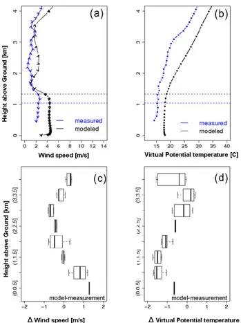
Vertical profiles of meteorological fields are validated for 2 to 30 August 2006 with the measurements provided by the Bayreuth wind profiler, located about 10 km south-west of OXK. For demonstration, a comparison of measured and modeled wind and temperature profiles on 3 August 2006 at 15:00 UTC is shown in Fig. 2a and b. The time period was chosen as representative for the model performance when the boundary layer is well-mixed. The observed prevailing wind direction was northerly for the atmospheric column below 2 km which was also reproduced by the model simulation. For a thin vertical layer, between 2.3 and 3.2 km, the prevail-ing wind direction changed to south-east; however the model simulated a north-westerly wind. Above 3.2 km, both ob-servations and simulations indicated a south-westerly wind. The magnitude of the wind was overestimated in the model, particularly in the boundary layer (bias: ∼+2 m s−1_).

A model-measurement comparison of the vertical profile of virtual potential temperature (θ v) showed an overestima-tion of simulated θ v. A relatively gradual increase in θ v (compared to simulations) was observed for the thin vertical layer between 2.3 and 3.2 km which could not be captured in the model. A possible reason for the decrease in θ v could be the intrusion of air from south-east direction on this layer (see Fig. 2a for wind direction) that existed for a short period of time.

To analyze the overall agreement, the monthly aver-ages of profiles for wind-speed and θ v, both measured and simulated, are produced at 15:00 UTC and the model-measurement mismatches are shown in Fig. 2c and d. The result shows that the model overestimated wind-speed in the boundary layer and in contrast showed a slight underestima-tion for the free troposphere. In general, the model slightly underestimated θ v profiles, particularly in the boundary layer. Overall, the model could capture much of the vari-ability in the vertical profiles of wind-speed and θ v.

3.1.2 Tower

Evaluations of the modeled meteorology are carried out at different measurement levels on the tower for different sea-sons. An example of those validations is demonstrated here. 1 2 3 4 5 6 7 8 9

Figure 2. (a-b) Profiles of observed vs. modeled wind fields and virtual potential

temperature for 3rd August 2006 at 15 UTC. The horizontal direction of wind is indicated with arrowheads. The dashed horizontal lines represent both observed (in blue) and simulated (in black) mixing heights calculated using bulk Richardson method. (c-d) the model-measurement mismatch for the monthly averages of these fields at 15 UTC, plotted against different altitude bins. The box indicates 95% quartile, the whisker denotes minimum and maximum of deviations and the vertical bar inside the box denotes the median.

Fig. 2. (a–b) Profiles of observed vs. modeled wind fields and

vir-tual potential temperature for 3 August 2006 at 15:00 UTC. The hor-izontal direction of wind is indicated with arrowheads. The dashed horizontal lines represent both observed (in blue) and simulated (in black) mixing heights calculated using bulk Richardson method.

(c–d) the model-measurement mismatch for the monthly averages

of these fields at 15:00 UTC, plotted against different altitude bins. The box indicates 95 % quartile, the whisker denotes minimum and maximum of deviations and the vertical bar inside the box denotes the median.

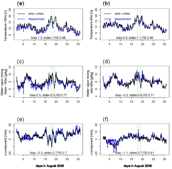
Figure 3 shows time series’ of observed and WRF-simulated variables (temperature, relative humidity and wind

compo-nents) for August 2006. The plot shows the prevailing

weather situation and also the model capability to predict these variables, which can drive atmospheric CO2

variabil-ity over OXK.

Simulated atmospheric temperatures at two different levels (90 m and 163 m) on the tower agree well with observations (squared correlation coefficient, R2=0.86 and bias = 0.8 to 1.3◦C) (Figs. 3a, b) and captured reasonably well the diurnal variability of temperature. Note that the model layers relative to the model terrain are used for all comparisons unless other-wise mentioned. This good temperature agreement suggests that uncertainties in the (simulated) temperature dependent VPRM respiration fluxes caused by temperature biases are expected to be small on synoptic time scales.

1

2

3

4

5

6

Figure 3. Comparison of measured and modeled meteorological parameters for August

2006 at the OXK site: (a-b) temperature at 163 m and 90 m, (c-d) water vapor mixing

ratio at 163 m and 90 m and (e-f) horizontal components of wind at 163 m. The green

dotted vertical lines denotes the passage of a cold front investigated in detail (see Sect.

4.1)

Fig. 3. Comparison of measured and modeled meteorological parameters for August 2006 at the OXK site: (a–b) temperature at 163 m and

90 m, (c–d) water vapor mixing ratio at 163 m and 90 m and (e-f) horizontal components of wind at 163 m. The green dotted vertical lines denotes the passage of a cold front investigated in detail (see Sect. 4.1).

The transport of moisture (comparable to CO2transport)

in the model was validated by comparing the measured and simulated water vapor mixing ratio at two levels. The model agrees well with the observations (R2=0.71 to 0.77) with slight biases (Figs. 3c and d).

The wind speed and direction was also predicted reason-ably well. A comparison of horizontal components of ob-served and modeled wind components u (east-west) and v (north-south) at 163 m (Figs. 3e and f) demonstrates fairly good agreement between observations and simulations (R2=

0.70 and 0.61 respectively).

Table 1 gives the overall model performance (model bias, standard deviation of model-measurement mismatch and squared correlation coefficient of the model-measurement agreement) from comparing the hourly time series of ob-served and simulated meteorological fields at the

avail-able measurement levels for different seasons. The sum-mary statistics indicate that WRF could follow the seasonal changes in the atmospheric transport and dynamics in most of the cases.

3.1.3 DIMO campaign

Vertical distributions of meteorological fields were validated against the DIMO profiles around the Ochsenkopf mountain region for all campaign days. The box-whisker plot (Figs. 4a, b) of the model-measurement mismatch (from all aircraft profiles) provides an overview of the model performance on simulating specific humidity and wind speed. In general, WRF meteorological simulations agree well with the DIMO observations as indicated by the lower median (+0.25 g kg−1 for water vapor mixing ratio and −0.06 m s−1for wind speed

Fig. 4. The box-whisker plot of model mismatch (simulations-observations) using all aircraft profiles for (a) specific humidity, (b) wind

speed and (c) CO2(WRF-VPRM) (d) CO2(STILT-VPRM).The box indicates 95 % quartile, the whisker denotes minimum and maximum

of deviations and the vertical bar inside the box denotes the median. Black dots are outliers.

Table 1. Summary statistics of observed and simulated (WRF) meteorological fields (model bias (bias), standard deviation of the difference

between the model and the data (sd) and squared correlation coefficient R2)using hourly time series at available measurement levels for different seasons. The bias and sd are in SI units of respective meteorological fields.

Season Level Temperature Water vapor mixing ratio u-component v-component

bias sd R2 bias sd R2 bias sd R2 bias sd R2

Spring 163 1.2 1.4 0.81 0.7 0.5 0.87 0.9 3.1 0.92 1.2 2.3 0.66 (May 2006) 90 0.7 1.3 0.80 0.2 0.7 0.66 – – – – – – Summer 163 1.3 1.0 0.86 0.5 0.5 0.77 0.3 2.7 0.70 1.1 2.7 0.61 (Aug 2006) 90 0.8 1.1 0.86 −0.3 0.6 0.71 – – – – – – Autumn 163 0.2 1.7 0.68 0.6 1.0 0.79 2.2 3.4 0.81 0.2 3.0 0.65 (Oct 2006) 90 −0.1 1.6 0.67 −0.1 1.1 0.73 – – – – – – Winter 163 1.4 0.9 0.93 0.2 0.4 0.88 0.6 6.4 0.48 1.2 5.0 0.33 (Mar 2008) 90 1.2 1.0 0.91 −0.1 0.5 0.81 – – – – – –

1

2

3

4

5

6

7

8

Figure 5. Vertical cross section (using a distance weighted interpolation) of the observed

and simulated meteorological fields as a function of distance flown by the aircraft for 19

October 2008: a-b) specific humidity in g/kg c-d) Wind speed in ms

. (a) and (c)

represent measurements and (b) and (d) represent WRF simulations. The grey lines

indicate flight track and the shaded grey region represents terrain elevation. See Figure 7d

for aircraft track showing altitude above ground. Time of the measurements/simulations

is given in the top X-axis.

Fig. 5. Vertical cross section (using a distance weighted interpolation) of the observed and simulated meteorological fields as a function

of distance flown by the aircraft for 19 October 2008: (a–b) specific humidity in g kg−1(c–d) Wind speed in m s−1. (a) and (c) represent measurements and (b) and (d) represent WRF simulations. The grey lines indicate flight track and the shaded grey region represents terrain elevation. See Fig. 7d for aircraft track showing altitude above ground. Time of the measurements/simulations is given in the top x-axis.

while using all available observations and simulations) and 95 % quartile (1.5 g kg−1for specific humidity and 3.2 m s−1 for wind speed). Noteworthy is that the model-measurement mismatch for water vapor mixing ratio increases with in-creasing height.

As an example, we demonstrate the model-measurement comparison for 19 October 2008 from 10:00 to 14:00 UTC. During this period, the air was sampled intensively near the top of OXK and the surrounding mountain ridges and val-leys (Fig. 5c). Figure 5 shows the vertical cross-section of the observed and modeled meteorological fields (wind speed and specific humidity) as a function of distance flown by the aircraft (Cumulative Distance, hereafter referred to simply as distance). WRF reproduced specific humidity fairly well at the surface layers; however, it showed an underestimation

in the upper vertical levels (Fig. 5a, b). A relatively calm wind (2 to 5 m s−1) was observed over Ochsenkopf moun-tain ranges during this period except in the early hours of the campaign. This was predicted well in WRF with negligible bias (Fig. 5c, d).

3.2 Model evaluation: CO2concentrations

Similar to Sect. 3.1, here we use observations of CO2fields

at OXK and during the DIMO aircraft campaign for the eval-uation of the models (WRF-VPRM and STILT-VPRM). As mentioned in the Sect. 1, we target at a monthly averaged flux uncertainty (in µmoles/(m2s−1)) with the upper bound-ary of 10 %. This flux criterion can abide a monthly averaged transport model bias of 0.4 to 0.6 ppm, which is obtained

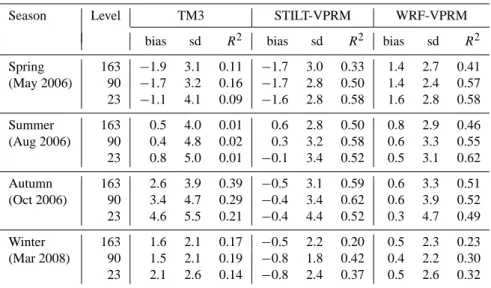
Table 2. Summary statistics of observed and simulated CO2fields (model bias (bias), standard deviation of the differences (sd) and squared

correlation coefficient R2)using 3-hourly time series at available measurement levels for different seasons. Simulated fields are provided by TM3, STILT-VPRM and WRF-VPRM. The bias and sd are in ppm units.

Season Level TM3 STILT-VPRM WRF-VPRM

bias sd R2 bias sd R2 bias sd R2

Spring 163 −1.9 3.1 0.11 −1.7 3.0 0.33 1.4 2.7 0.41 (May 2006) 90 −1.7 3.2 0.16 −1.7 2.8 0.50 1.4 2.4 0.57 23 −1.1 4.1 0.09 −1.6 2.8 0.58 1.6 2.8 0.58 Summer 163 0.5 4.0 0.01 0.6 2.8 0.50 0.8 2.9 0.46 (Aug 2006) 90 0.4 4.8 0.02 0.3 3.2 0.58 0.6 3.3 0.55 23 0.8 5.0 0.01 −0.1 3.4 0.52 0.5 3.1 0.62 Autumn 163 2.6 3.9 0.39 −0.5 3.1 0.59 0.6 3.3 0.51 (Oct 2006) 90 3.4 4.7 0.29 −0.4 3.4 0.62 0.6 3.9 0.52 23 4.6 5.5 0.21 −0.4 4.4 0.52 0.3 4.7 0.49 Winter 163 1.6 2.1 0.17 −0.5 2.2 0.20 0.5 2.3 0.23 (Mar 2008) 90 1.5 2.1 0.19 −0.8 1.8 0.42 0.4 2.2 0.30 23 2.1 2.6 0.14 −0.8 2.4 0.37 0.5 2.6 0.32 1 2 3 4

Figure 6. Comparison of measured and modeled CO2 concentrations for August 2006 at

90 m on the OXK. A period between dashed green vertical bars denotes a synoptic event during 0 to 15 UTC on 18th _{August 2006 (see also Sect. 4.1)}

Fig. 6. Comparison of measured and modeled CO2

concentra-tions for August 2006 at 90 m on the OXK. A period between dashed green vertical bars denotes a synoptic event during 00:00 to 15:00 UTC on 18 August 2006 (see also Sect. 4.1).

by transporting biospheric CO2 fluxes from uptake (gross

ecosystem exchange) or release (ecosystem respiration) dur-ing the growdur-ing period with an additional flux uncertainty of 10 % on a monthly scale.

3.2.1 Tower

The observed atmospheric CO2 concentrations at different

measurement levels are compared with simulations gener-ated by WRF-VPRM and STILT-VPRM for different sea-sons. For illustration, we show the time series comparison of CO2concentrations at 90 m level on the tower for the period

from 2 to 30 August 2006 (Fig. 6). The period is chosen due

to its enhanced biospheric activity and the existence of strong diurnal patterns in transport and fluxes which can complicate the measurement interpretation. For comparison, the CO2

analyzed fields from TM3 with 3-hourly time steps are also

included. The observed atmospheric CO2 shows large

di-urnal and synoptic variability and notably, these large

vari-ations in atmospheric CO2 were not captured in the TM3

global model. Note that the generation of analyzed CO2

fields (by atmospheric inversion) did not include OXK CO2

data, so in this sense they can be used for independent vali-dation. The comparison becomes more favorable when high-resolution transport and fluxes are used. Most of the ob-served temporal patterns in CO2concentrations on the tower

is reproduced remarkably well in both high-resolution mod-els (R2=0.55 to 0.58) when compared to TM3 (R2=0.02, see Fig. 6). The high-resolution models slightly overesti-mated the CO2concentrations with biases ranging from 0.3

to 0.6 ppm (Table 2), which is in the targeted range (10 %) of the monthly averaged flux uncertainty. The better per-formance of high-resolution models points to the fact that most of the variations in CO2 are due to surface flux

vari-ations and mesoscale transport processes on scales not re-solved by TM3, which has a grid-cell size of several hundred kilometers. Also note that TM3 uses coarse resolution terrain elevation data.

In addition to August (summer) 2006, CO2concentrations

are also validated for other seasons and the summary statis-tics (similar to Table 1) of the model-measurement compar-ison are given in Table 2. Observations from other levels (23 m and 163 m) on the tower are also used to assess the models’ performance in reproducing the vertical structure of CO2in the atmospheric column. The summary statistics

clearly indicate that high-resolution models are able to pre-dict reasonably well the temporal patterns of CO2(measured

at three different vertical levels on the tower) for different seasons when compared to the coarse resolution model. Sec-tion 3.2.4 discusses further the seasonal variability of CO2

concentrations.

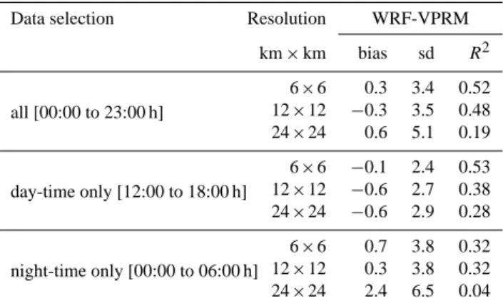
In this context, it is interesting to assess what is the minimum spatial resolution of the model which is required

to represent OXK (CO2) measurements that would

en-able to design the future regional inversion system at the lowest possible computational requirements. This assess-ment was accomplished by performing WRF-VPRM simu-lations at different spatial resolutions such as 6 km × 6 km, 12 km × 12 km and 24 km × 24 km and by evaluating those simulations against measurements. Table 3 gives the sum-mary statistics of the model performance. The result indi-cates that there is a strong degradation of the model per-formance when decreasing the model spatial resolution to 24 km, compared to 6 km (100 % increment in model bias, 46 % increment in standard deviation of the difference and 150 % reduction in squared correlation coefficient). The model at 24 km resolution could not capture most of the noc-turnal variability as compared to higher resolutions. The sim-ulations from other resolutions (6 km and 12 km) can be ar-gued to be of similar quality in most of the cases. This sug-gests that a minimum spatial resolution of 12 km is required

to represent OXK CO2measurements.

3.2.2 DIMO campaign

The profiles of atmospheric CO2 concentrations obtained

from the aircraft campaign were used to examine how well the models can reproduce the vertical distribution of tracer concentrations over the Ochsenkopf mountain region. Fig-ure 4c shows the statistical analysis of model-measFig-urement mismatches using CO2profiles for all days in the campaign.

The median of all residuals is 0.5 (1.1) ppm for STILT-VPRM (WRF-STILT-VPRM). The model-measurement mismatch of CO2 for both models increases with decreasing heights,

the opposite of what was found for water vapor. The rea-sons can be: (1) the large variability of CO2at the surface

compared to higher levels (Pillai et al., 2010), (2) improper representation of boundary layer vertical mixing in the mod-els and, (3) water vapor has sinks (precipitation) in the atmo-sphere, while CO2has not.

The same period that was chosen for DIMO meteorologi-cal validations is used also here as an example to demonstrate the vertical distribution of CO2. Figure 7 shows the vertical

cross section of the observed and simulated CO2

concentra-tion as a funcconcentra-tion of distance for 19 October 2008 from 10:00 to 14:00 UTC. Compared to summer months, higher values of CO2are generally expected due to lower biosphere uptake

and shallower vertical mixing. Accumulation of CO2in the

valley south of OXK was observed in the morning (10:30– 11:30 UTC) between the aircraft’s cumulative flown distance

Table 3. Summary statistics of observed and simulated CO2fields

for various model resolutions. The statistics includes model bias (bias), standard deviation of the differences (sd) and squared cor-relation coefficient (R2)which are calculated using 3-hourly time series data, separately for different data selections for the measure-ment level at 23 m during August 2006. Simulated fields are gener-ated by WRF-VPRM. The bias and sd are in ppm units.

Data selection Resolution WRF-VPRM km × km bias sd R2 all [00:00 to 23:00 h] 6 × 6 0.3 3.4 0.52 12 × 12 −0.3 3.5 0.48 24 × 24 0.6 5.1 0.19 day-time only [12:00 to 18:00 h] 6 × 6 −0.1 2.4 0.53 12 × 12 −0.6 2.7 0.38 24 × 24 −0.6 2.9 0.28 night-time only [00:00 to 06:00 h] 6 × 6 0.7 3.8 0.32 12 × 12 0.3 3.8 0.32 24 × 24 2.4 6.5 0.04

range 120 and 200 km (see Fig. 7a). CO2can accumulate in

valleys under shallow vertical mixing in the nocturnal bound-ary layer as well as under nocturnal drainage conditions in complex terrain. The valley-mountain gradient in CO2

concentrations in the valley decreased rapidly in the after-noon with the establishment of convective mixing and con-sequently enhanced vertical turbulence. STILT-VPRM and

WRF-VPRM were able to capture relatively well the CO2

accumulation in the valley in the morning (distance between 100 and 200 km); however WRF-VPRM slightly underesti-mated the vertical extent of valley accumulation during this period. At noon (distance between 280 and 320 km), STILT-VPRM overestimated the CO2concentrations and this

over-estimation can also be seen in the afternoon when the bound-ary layer is well mixed.

4 Discussion

4.1 Synoptic variability

The observations show considerable synoptic variability in CO2concentrations which are driven by atmospheric

trans-port and surface flux heterogeneity. These synoptic varia-tions in tracer concentravaria-tions provide valuable information on spatiotemporal patterns of surface fluxes and thus can be used in atmospheric inversion to construct regional fluxes. A synoptic event (cold front), observed on 18 August 2006,

during which the observed CO2showed an enhancement of

more than 20 ppm, is analyzed in detail to examine how such variations are represented by the mesoscale models. In the beginning of the event, the air temperature dropped signifi-cantly with a relatively sharp increase in humidity (Fig. 3a

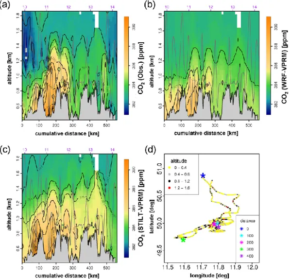
Fig. 7. Vertical cross section (using a distance weighted interpolation) of the observed and simulated CO2fields (given in ppm) as a function

of distance flown by the aircraft (cumulative distance) for 19 October 2008: (a) measurements (b) WRF-VPRM (c) STILT-VPRM and

(d) Flight track with color gradient showing altitude range (legend at the top left-hand side of the panel) above ground. The symbol “*”

denotes cumulative distance in km (legend at the bottom right-hand side of the panel). In (a–c), the time of measurements/simulations is given in the top x-axis.

to d). The wind speed was relatively high, reaching a maxi-mum of 15 m s−1. The atmospheric CO2observation shows

a large peak during this period, which was captured by both models as seen in Figs. 6, 8a and 8b. However the mod-els predict this elevated concentration with a considerable low bias of ∼15 ppm. During the event, the air was coming from the south-west, and the time integrated footprints de-rived from STILT (sensitivity of mixing ratio at 07:00 UTC on 18 August to surface fluxes integrated over the past 48 h), shows a strong influence from the highly industrialized area in the south-west part of Germany occurring 10 h prior to the measurement (Fig. 8c). Tracer simulations, where an-thropogenic and biospheric contributions within the domain are separated, show a large contribution from respiration and emission fluxes for the event (Fig. 8a) and consequently an

increase in CO2concentration in the atmosphere (Fig. 8b),

which reached a peak in the early morning, owing to the shal-low mixing in the nocturnal boundary layer. These higher concentrations started decreasing with the development of the convective mixed layer combined with the drawdown of CO2 by photosynthesis. The above analysis suggests that

OXK during this event was highly influenced by air carry-ing a large contribution from respiration, but also emissions originating from densely populated and industrialized area. The underestimation of the CO2 peak in the models could

be due to several reasons: (1) uncertainties in vertical mixing (this is the more likely scenario as it would strongly affect the vertical distribution of tracer concentrations, producing large model-measurement mismatches) (2) uncertainties in advec-tion (WRF underestimated the wind speed in the beginning

1 1 2 3 4 5 6 7

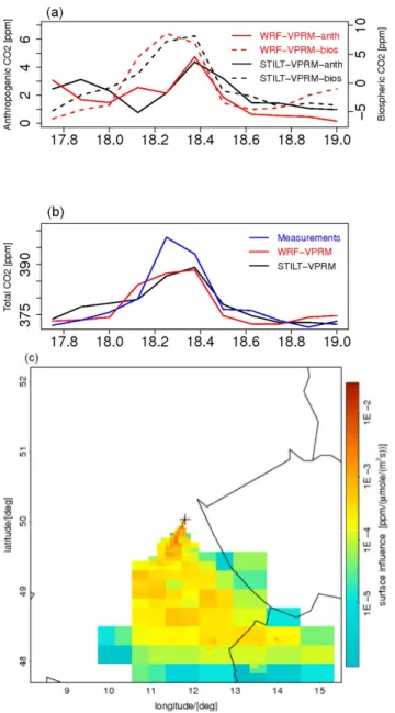
Figure 8. Influence of surface fluxes on measured CO2 concentration at OXK: a and b)

Time series of simulated anthropogenic and biospheric CO2 signals (contribution of

anthropogenic and biospheric fluxes to the total CO2) at 90 m on the tower during 17-18

August 2006. c) Time integrated footprints derived by STILT on 18th August 2006 at 7:00 UTC for particles running -48 hours (backward in time) from tower (indicated with + sign)

Fig. 8. Influence of surface fluxes on measured CO2

concentra-tion at OXK: (a) and (b) Time series of simulated anthropogenic and biospheric CO2signals (contribution of anthropogenic and

bio-spheric fluxes to the total CO₂)at 90 m on the tower during 17– 18 August 2006. (c) Time integrated footprints derived by STILT on 18 August 2006 at 07:00 UTC for particles running −48 h (back-ward in time) from tower (indicated with + sign).

of the event and predicted south-easterly wind rather than the observed westerly wind direction. The strong south-westerly wind might be associated with advection of large

plumes of CO2 (respired and anthropogenic) to the

mea-surement location) (3) the underestimation of anthropogenic emissions in the inventory for this area of influence (uncer-tainties of emission inventories at small spatial and short tem-poral scales can easily be as large as 50 % (Olivier et al., 1999) (4) uncertainties in the VPRM respiration fluxes (note

that VPRM simulates respiration fluxes as a linear function of the simulated surface temperature (at 2 m). The uncer-tainty due to a temperature bias is likely to be small because the simulated temperature for this period is fairly in good agreement with observations. However, the respiration fluxes in reality are not only controlled by temperature but also by other factors such as soil moisture.) (5) underestimation of TM3 initial fields (it is more unlikely that a short term event, which originated outside of Europe domain, would have had an influence on this). This emphasizes the complexities of mechanisms involved in such short-term scale events. The vertical profiling of CO2 (as like DIMO aircraft campaign)

or wind profiler measurements can be helpful to assess the impact of vertical mixing on tracer concentrations).

In general, both high-resolution models could capture the general trend of CO2variability during this synoptic event,

by simulating well the influence of surface fluxes in the near-field and the atmosphere dynamics.

4.2 Orographic effect

The mountainous terrain can influence the regional circula-tion pattern around the tower site, resulting in local flow pat-terns which can have an impact on diurnal patpat-terns in tracer concentration measurements. The local flow patterns are de-veloped by the formation of (1) thermally forced mountain-valley circulations in response to radiative heating and cool-ing of the surface and (2) topographically induced stationary gravity waves (i.e., mountain waves) when stable flow en-counters a mountain barrier. The downslope flows are more common at OXK during nighttime although mountain grav-ity waves are also likely in winter periods (based on WRF simulations as well as photographs taken during DIMO cam-paign).

4.2.1 Mountain-valley circulations

The mountain valley flows can change the atmospheric ver-tical mixing and can thus influence tracer measurements at OXK (Thompson et al., 2009). An example of such an event occurred at nighttime between 26 and 27 August 2006 is demonstrated in Fig. 9. During this period, the expected nocturnal CO2build up at OXK was found to be nearly

ab-sent owing to the thermally induced drainage flow. The data shown are the time series of meteorological and CO2

ob-servations at each level on the tower for a period from 26 to 28 August 2006. The period between the brown vertical dashed lines in Fig. 9 shows evidence of mountain-valley cir-culation. Also the period was under weak synoptic pressure gradient conditions (as indicated by the simulated potential temperature) with a prevailing westerly flow (as indicated by the simulated wind speed) (Fig.10a, c). The observed tem-perature and wind speed during this period (Fig .9a, b) also suggest that the conditions were favorable for the formation of a buoyancy-driven downslope flow. Following radiative

1

2

3

4

5

6

7

8

Figure 9. Time series of meteorological parameters and CO

concentrations for different

levels at OXK site during 26-28 August 2006: a-c) observed air-temperature, relative

humidity and wind speed respectively d-f) CO

concentration, observed and modeled by

WRF and STILT, respectively. The area between dashed brown vertical bars denotes the

period under mountain-valley circulation. The X-axis shows hours in UTC; the horizontal

extent of curly bracket at the bottom of X-axis shows the day on August 2006.

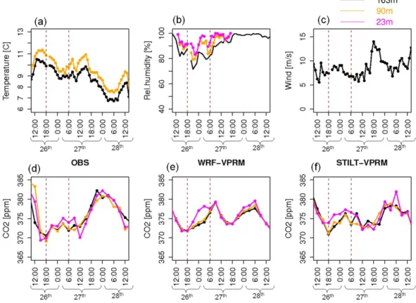
Fig. 9. Time series of meteorological parameters and CO2concentrations for different levels at OXK site during 26–28 August 2006:

(a–c) observed air-temperature, relative humidity and wind speed respectively (d–f) CO2concentration, observed and modeled by WRF and

STILT, respectively. The area between dashed brown vertical bars denotes the period under mountain-valley circulation. The x-axis shows hours in UTC; the horizontal extent of curly bracket at the bottom of x-axis shows the day on August 2006.

cooling of the surface on 26 August, relatively dry air in-truded from the free troposphere into the nocturnal boundary layer, which was observed as a sharp decrease in the rela-tive humidity (Fig. 9b). Noticeable time lags in the transi-tion from moist to dry air were seen at the different sampling levels, which also indicate the intrusion of air from above. The evidence of dry air subsidence from the residual layer can also be seen later at 06:00 UTC on 27 August. Conse-quently, a decrease in CO2 concentration was observed at

00:00 UTC and at 06:00 UTC on 27 August due to the re-placement of air by the residual layer containing lower CO2

concentration. STILT-VPRM captured well the lowering of CO2concentration at 06:00 UTC in response to the drainage

flow and simulated well-mixed tracer concentrations in the nocturnal boundary layer. However WRF-VPRM showed an unrealistic accumulation of CO2concentration at the lower

level which might be associated with the underestimation in the vertical extent of the entrainment air reaching the tower site. The presence of katabatic flow on the lee side of the mountain was predicted in WRF, indicated by the negative vertical velocity (downward movement of air) and increased wind speed along the mountain slope (Fig. 10d). The (sim-ulated) impact of drainage flow on the tracer concentrations

on the lee side of the mountain can be seen as a region of lower CO2contours in Fig. 10b.

4.2.2 Mountain wave activity

The buoyancy driven upslope and downslope flows, which are discussed above, are less common in winter due to low surface heating. As mentioned earlier, under stable strati-fied nocturnal boundary conditions, mountain gravity waves can be formed when air flow is perturbed with a barrier (e.g. mountain). Propagation of gravity waves transport-ing mass and energy in the stable boundary layer can af-fect tracer concentrations measured at the tower. The pos-sible occurrence of gravity waves can be assessed by esti-mating the Froude number (Stull, 1988), Fr (the ratio of in-ertial to gravitational forces, =

U

(N ×h)_{) which relates the}

pre-vailing horizontal wind speed (U ), mountain height (h) and buoyancy oscillation frequency (Brunt-V¨ais¨al¨a frequency,

N-calculated as a function of potential temperature). When Fr is near unity, the wavelength of the air flow is in resonance with the mountain size, creating trapped mountain lee waves which results in strong downslope winds and enhanced tur-bulence on the lee side of the mountain.

1

2

3

4

5

6

Figure 10. Vertical cross section along OXK latitude (50

01" N) on 27

August 2006 at

01:00 UTC, showing WRF-VPRM simulated a) Potential temperature in Kelvin b) CO

concentration in ppm c) Wind speed in ms

and d) Vertical velocity in ms

The overlaid

arrows indicate prevailed wind direction at different altitudes; the symbol “+” indicates

OXK location.

Fig. 10. Vertical cross section along OXK latitude (50◦01” N) on 27 August 2006 at 01:00 UTC, showing WRF-VPRM simulated (a) Poten-tial temperature in Kelvin (b) CO2concentration in ppm (c) Wind speed in m s−1and (d) Vertical velocity in m s−1. The overlaid arrows

indicate prevailed wind direction at different altitudes; the symbol “+” indicates OXK location.

However, the mountain wave activity is much more com-plex in reality and is difficult to interpret its effects on measurements. An ideal case of such an activity was oc-curred at a nighttime between 16 and 17 October 2006 (be-tween brown dashed lines in Fig. 11). A temperature in-version was observed during this period (Fig. 11a) indicat-ing the stable atmospheric conditions. The sharp decrease in observed relative humidity on the tower under relatively high wind speed indicates the presence of possible moun-tain wave activity with intrusion of dry air on the lee side of the mountain. These meteorological features were predicted reasonably well by the WRF model and the west-east cross section of simulated vertical velocity shows the downward movement of air at the lee side of the mountain (Fig. 12d). Note that the WRF simulations might not always capture the waves correctly and the caution has to be taken to interpret the structures of the vertical velocity fields which can also be formed due to the numerical noise. The increased gradient in the simulated potential temperature, together with higher values of simulated vertical velocity (50 cm s−1)and strong wind speed, suggests the occurrence of mountain wave

phe-nomena at the OXK site (Fig. 12). The Froude number was found to be close to unity, indicating the likelihood of gravity wave (mountain wave) activity. In addition to this, the sim-ulated wavelengths λ(=U_N)for the region over the mountain were found to be close to the mountain height, showing the existence of vertically propagating mountain waves.

Following the collapse of the convective boundary layer on 16 October, CO2started to build up in the nocturnal shallow

boundary layer and showed a distinctive gradient between layers for a few hours between 18:00–21:00 UTC. These

nocturnal developments of CO2 were captured in

STILT-VPRM; however the vertical mixing between levels at 23 m and 90 m was underestimated. Corresponding to the pre-vailing mesoscale feature, the observed nocturnal gradient in tracer concentrations disappeared in response to the de-cent of air from the free troposphere. This was reproduced well in STILT-VPRM, while WRF-VPRM showed the de-creasing tendency of CO2concentrations on this period but

with an unrealistic gradient between the layers (00:00 to 06:00 UTC during 16–17 October 2006), which might be due to the underestimated mixing process. Note that vertical

1

2

3

4

5

6

7

8

Figure 11. Time series of meteorological parameters and CO2

concentrations for

different levels at Ochsenkopf tower site during 16-17 October 2006: a-c) observed

air-temperature, relative humidity and wind speed respectively d-f) CO

concentration-observed, modeled by WRF and STILT respectively. The area between dashed brown

vertical bars denotes the period under mountain wave activity. The X-axis shows hours in

UTC; the horizontal extent of curly bracket at the bottom of X-axis shows the day on

October 2006.

Fig. 11. Time series of meteorological parameters and CO2concentrations for different levels at Ochsenkopf tower site during 16–17

Oc-tober 2006: (a–c) observed air-temperature, relative humidity and wind speed respectively (d–f) CO2concentration-observed, modeled by

WRF and STILT respectively. The area between dashed brown vertical bars denotes the period under mountain wave activity. The x-axis shows hours in UTC; the horizontal extent of curly bracket at the bottom of x-axis shows the day on October 2006.

mixing is parameterized slightly differently in WRF-VPRM and STILT-VPRM. The influence of mountain waves on gen-erating turbulent vertical mixing of nocturnal tracer concen-trations at the lee side of the valley can be seen in the WRF-VPRM simulations (Fig. 12b). Owing to the strong down-ward movement of air and vertical mixing, a layer of lower CO2 concentration was simulated for the western slope of

the mountain, despite the nocturnal build-up period. The nocturnal build-up of CO2 under shallow mixing and weak

biological CO2 uptake were simulated for the other valleys

(Fig. 12b).

The above two case studies suggest that changes in the atmospheric transport and mixing in response to mesoscale phenomena, such as mountain-valley circulations and moun-tain wave activities, can strongly affect the diurnal patterns of CO2concentrations at OXK, and that these can be

repre-sented well in mesoscale models at the resolution of 2 km. 4.3 Seasonal variability

Different seasonal aspects, such as changes in thermal cir-culation patterns (changes in solar radiation), changes in di-urnal patterns of vertical mixing, effects of snow cover and

diurnal variations in surface fluxes, can have an important in-fluence on measured tracer concentrations. Seasonal changes in the diurnal patterns of CO2concentration are observed at

Ochsenkopf mountain station as it can be influenced by het-erogeneous land sources and sinks as well as by synoptic atmospheric conditions. Figure 13 shows averaged diurnal cycles of observed and modeled CO2at different

measure-ment levels and for different seasons. Except for the level 163 m in winter and autumn, the CO2concentration maxima

were observed during nighttime due to the accumulation of CO2concentration in the shallow nocturnal boundary layer.

The measurement level at 163 m during winter and autumn is more representative of free tropospheric or residual layer air, as indicated by the weak diurnal changes in observed concentrations and by the decoupling relative to the lower levels. The slight daytime increase at the 163 m level, de-layed by about six hours compared to the lower levels, is consistent with the daytime mixing of air previously trapped in the stable mixed layer, containing remnants of respired CO2 from the previous night. The amplitude of the

diur-nal cycle is larger in spring and summer months (∼8 ppm), consistent with the enhanced biospheric activity (photosyn-thesis and ecosystem respiration), whereas the amplitude is

1

2

3

4

5

6

Figure 12. Vertical cross section along OXK latitude (50

01" N) on 17

October 2006 at

02:00 UTC, showing WRF-VPRM simulated a) Potential temperature in Kelvin b) CO

concentration in ppm c) Wind speed in ms

and d) Vertical velocity in ms

The overlaid

arrows indicate wind direction at different altitudes.

Fig. 12. Vertical cross section along OXK latitude (50◦01” N) on 17 October 2006 at 02:00 UTC, showing WRF-VPRM simulated (a) Po-tential temperature in Kelvin (b) CO2concentration in ppm (c) Wind speed in m s−1and (d) Vertical velocity in m s−1. The overlaid arrows

indicate wind direction at different altitudes.

smaller in autumn and winter months owing to the reduced diurnal variability in the terrestrial fluxes. The low values of CO2are noticeable in August (active growing season) due to

enhanced biospheric CO2uptake. The model-measurement

agreement is fairly good for higher resolution models, except for the level 163 m in winter and autumn seasons where both models overestimate the vertical mixing. The coarse resolu-tion TM3 analyzed CO2fields (taken from 940 hectopascal

(hPa) TM3 pressure level which corresponds to the measure-ment levels above sea level, i.e. relative to the sea level; indi-cated as “TM3” in Fig. 13) show little diurnal change during all seasons and at all levels. On the other hand, TM3 an-alyzed CO2 fields corresponding to the model levels close

to the measurement levels from the surface, i.e. relative to the model terrain (taken from 1013 hPa and 1002 hPa TM3 pressure levels corresponding to the levels on the tower; in-dicated as “TM3-surface” in Fig. 13) show large diurnal vari-ability due to the strong influence of surface fluxes near the ground, but with large positive biases in most of the cases. This discrepancy can lead to potential biases in flux

esti-mates when using measurements from a site like OXK, as discussed above. Again, this suggests the importance of us-ing high-resolution models to resolve the large variability of atmospheric CO2concentrations in response to variability in

surface fluxes and mesoscale transport. In order to examine whether the poor performances of TM3 are caused by the coarse resolution flux fields (horizontal resolution: 4◦×5◦), we run STILT-VPRM with biospheric fluxes aggregated to

∼500 km × 500 km resolution, comparable to the TM3 res-olution. CO2 simulated by this coarse resolution version

of STILT-VPRM shows remarkable similarity to the high-resolution simulations by STILT and WRF in the diurnal cy-cle for the different seasons.

4.4 Vertical distribution of CO2concentrations

The vertical profiling of atmospheric CO2 during aircraft

campaigns provides more information on vertical mixing in the atmosphere and provide the opportunity to evaluate cur-rent transport models. The discrepancies in predicting at-mospheric mixing can lead to a strong bias in the simulated

1

2

Fig. 13. Averaged diurnal cycle of observed and modeled CO2for OXK at different measurement levels and for different seasons: (a) May

2006 (spring), (b) August 2006 (summer), (c) October 2006 (autumn) and (d) March 2008 (winter). In each plots, top to bottom panels represents CO2at 163 m, 90 m and 23 m respectively. x-axis: hour; y-axis: CO2concentration in ppm.

vertical distribution of CO2concentrations. An example of

such an effect can be seen in Figs. 5 and 7. The underestima-tion of the vertical extent of CO2accumulation (as mentioned

in Sect. 3.2.2, Fig. 11a, b) can be caused by the overestima-tion of vertical mixing in WRF. The effect of this overes-timation can also be seen in the modeled specific humidity

(Fig. 5b) as low values (underestimation) in the upper layers. Note that the wind speed was predicted well in WRF with negligible bias.

It should also be mentioned that the difference in observed and modeled wind speed found at the Ochsenkopf valley for another day of the campaign (23 October 2008) generated an

underestimation of CO2concentration in both WRF-VPRM

and STILT-VPRM (figure not shown). WRF underestimated the flow of air, advected from upstream locations and con-sequently failed to capture the huge contribution of the ad-vected respired signal to the measurement locations. STILT-VPRM also shows a similar underestimation of CO2

concen-tration for the same reason.

These two case studies of model evaluation with the air-borne measurements show the necessity of accurately pre-dicting the mesoscale atmospheric transport, such as advec-tion and convecadvec-tion, as well as vertical mixing. Both mod-els are able to capture the spatial variability of measured CO2 concentration in the complex terrain for most of the

cases and the discrepancy between models and measure-ments are mainly attributed to the difference in representing atmospheric PBL dynamics.

5 Summary and conclusions

High-resolution modeling simulations of meteorological

fields and atmospheric CO2 concentrations, provided by

WRF-VPRM and STILT-VPRM, are presented together with measurements obtained from the Ochsenkopf tower (OXK) and from an aircraft campaign, to address the representative-ness of greenhouse gas measurements over a complex terrain associated with surrounding mountain ranges. The spatial and temporal patterns of CO2are reproduced well in

high-resolution models for different seasons when compared to the coarse model (TM3). This emphasizes the importance of using high-resolution modeling tools in inverse frameworks, since a small deviation in CO2concentration can lead to

po-tentially large biases in flux estimates. The actual reduction in uncertainties of flux estimates when using high-resolution models (compared to lower-resolution models) in the inverse framework needs to be further investigated.

The measurements of CO2at OXK show diurnal,

synop-tic and seasonal variability of CO2due to different aspects

such as changes in the diurnal patterns of vertical mixing, diurnal variations in surface fluxes, effect of front passage, changes in thermal circulation patterns etc. These variations in tracer concentrations provide valuable information on spa-tiotemporal patterns of surface fluxes and thus can be used in atmospheric inversions to construct regional fluxes. Both high-resolution models were able to capture this variability by simulating well the influence of surface fluxes in the near-field and the atmosphere dynamics. The model performance is assessed using a criterion of targeted monthly averaged flux uncertainty of 10 %.

The mesoscale flows, such as mountain wave activity and mountain-valley circulations, can have a strong influence on the observed atmospheric CO2at OXK by changing the

ver-tical mixing of the tracer concentrations. The meteorolog-ical simulations by WRF indicate that the buoyancy driven drainage flows are more common at OXK during nighttimes

(especially in summer) and mountain gravity waves are likely to occur in winter periods. Resolving these circulation pat-terns in models is a prerequisite for utilizing observations from mountain stations such as OXK with a reduced repre-sentation error.

The discrepancies in predicting vertical mixing can lead to strong biases in simulated CO2concentrations and these

kinds of uncertainties are typical for complex terrain regions. The vertical profiling of CO2(like the DIMO aircraft

cam-paign) or wind profiler measurements can be helpful in as-sessing the impact of vertical mixing on tracer concentra-tions. Our study shows that much of the variability in CO2

concentrations can be reproduced well by appropriate rep-resentation of mesoscale transport processes, such as advec-tion, convection and vertical mixing as well as surface flux influences in the near-field.

This study demonstrates the potential of using high-resolution models in the context of inverse modeling frame-works to utilize measurements provided from mountain or complex terrain sites. The model evaluation of different spa-tial resolutions suggests that a minimum resolution of 12 km is required to represent OXK mountain station. Our future work will focus on regional inversions using STILT-VPRM at the required resolution (e.g. 10 km × 10 km) with a nested option. The feasibility of using these high- resolution nests in global models has already been demonstrated by (R¨odenbeck et al., 2009). This provides justified hope that measurements from mountain stations can be utilized in inverse modeling frameworks to derive regional CO2budgets at reduced

un-certainty limits.

Acknowledgements. We thank Martin Heimann, Max Planck

Institute of Biogeochemistry, Germany for continuing support and helpful discussions. We acknowledge Deutscher Wetterdienst (DWD), Germany for providing wind profiler data. We are also thankful to the whole Ochsenkopf tall tower team in Max Planck Institute of Biogeochemistry, Germany for their assistance in data processing.

The service charges for this open access publication have been covered by the Max Planck Society. Edited by: P. Monks

References

Ahmadov, R., Gerbig, C., Kretschmer, R., Koerner, S., Neininger, B., Dolman, A. J., and Sarrat, C.: Mesoscale covariance of transport and CO₂ fluxes: Evidence from observations and simulations using the WRF-VPRM coupled atmosphere-biosphere model, J. Geophys. Res.-Atmos., 112, D22107, doi:22110.21029/22007JD008552, 2007.

Ahmadov, R., Gerbig, C., Kretschmer, R., Krner, S., Rdenbeck, C., Bousquet, P., and Ramonet, M.: Comparing high resolution WRF-VPRM simulations and two global CO2 transport

mod-els with coastal tower measurements of CO₂, Biogeosciences, 6, 807–817, doi:10.5194/bg-6-807-2009, 2009.