Optimal use of statistical methods to validate reference gene stability in longitudinal studies

HAL Id: inserm-02264433

https://www.hal.inserm.fr/inserm-02264433

Submitted on 7 Aug 2019

HAL is a multi-disciplinary open access archive for the deposit and dissemination of sci-entific research documents, whether they are pub-lished or not. The documents may come from teaching and research institutions in France or abroad, or from public or private research centers.

L’archive ouverte pluridisciplinaire HAL, est destinée au dépôt et à la diffusion de documents scientifiques de niveau recherche, publiés ou non, émanant des établissements d’enseignement et de recherche français ou étrangers, des laboratoires publics ou privés.

gene stability in longitudinal studies

Venkat Krishnan Sundaram, Nirmal Kumar Sampathkumar, Charbel

Massaad, Julien Grenier

To cite this version:

Venkat Krishnan Sundaram, Nirmal Kumar Sampathkumar, Charbel Massaad, Julien Grenier. Op-timal use of statistical methods to validate reference gene stability in longitudinal studies. PLoS ONE, Public Library of Science, 2019, 14 (7), pp.e0219440. �10.1371/journal.pone.0219440�. �inserm-02264433�

Multiple statistical approaches have been proposed to validate reference genes in qPCR assays. However, conflicting results from these statistical methods pose a major hurdle in the choice of the best reference genes. Recent studies have proposed the use of at least three different methods but there is no consensus on how to interpret conflicting results. Researchers resort to averaging the stability ranks assessed by different approaches or attributing a weighted rank to candidate genes. However, we report here that the suitability of these validation methods can be influenced by the experimental setting. Therefore, aver-aging the ranks can lead to suboptimal assessment of stable reference genes if the method used is not suitable for analysis. As the respective approaches of these statistical methods are different, a clear understanding of the fundamental assumptions and the parameters that influence the calculation of reference gene stability is necessary. In this study, the stabil-ity of 10 candidate reference genes (Actb, Gapdh, Tbp, Sdha, Pgk1, Ppia, Rpl13a, Hsp60,

Mrpl10, Rps26) was assessed using four common statistical approaches (GeNorm,

Norm-Finder, Coefficient of Variation or CV analysis and PairwiseΔCt method) in a longitudinal experimental setting. We used the development of the cerebellum and the spinal cord of mice as a model to assess the suitability of these statistical methods for reference gene vali-dation. GeNorm and the PairwiseΔCt were found to be ill suited due to a fundamental assumption in their stability calculations. Highly correlated genes were given better stability ranks despite significant overall variation. NormFinder fares better but the presence of highly variable genes influences the ranking of all genes because of the algorithm’s con-struct. CV analysis estimates overall variation, but it fails to consider variation across groups. We thus highlight the assumptions and potential pitfalls of each method using our longitudinal data. Based on our results, we have devised a workflow combining NormFinder, CV analysis along with visual representation of mRNA fold changes and one-way ANOVA for validating reference genes in longitudinal studies. This workflow proves to be more robust than any of these methods used individually.

a1111111111 a1111111111 a1111111111 a1111111111 a1111111111 OPEN ACCESS

Citation: Sundaram VK, Sampathkumar NK, Massaad C, Grenier J (2019) Optimal use of statistical methods to validate reference gene stability in longitudinal studies. PLoS ONE 14(7): e0219440.https://doi.org/10.1371/journal. pone.0219440

Editor: Bjoern Peters, La Jolla Institute for Allergy and Immunology, UNITED STATES

Received: February 25, 2019 Accepted: June 24, 2019 Published: July 23, 2019

Copyright:© 2019 Sundaram et al. This is an open access article distributed under the terms of the

Creative Commons Attribution License, which permits unrestricted use, distribution, and reproduction in any medium, provided the original author and source are credited.

Data Availability Statement: All relevant data are within the manuscript and its Supporting Information files.

Funding: The author(s) received no specific funding for this work.

Competing interests: The authors have declared that no competing interests exist.

Introduction

Relative expression of target genes in qPCR assays require accurate normalization of mRNA quantities using stably expressed internal standards also called reference genes [1]. In theory, such a gene is presumed to be stably expressed across all groups and samples [2]. This is sel-dom the case. There is no universal reference gene that fulfils this criterion and the choice of a good reference becomes highly subjective depending on several factors such as the sample/tis-sue type, experimental condition and sample integrity [3,4]. Many statistical methods have been proposed to help researchers identify stable reference genes from a predetermined set of candidates. These statistical approaches determine the stability of these candidates based on a unique set of assumptions and calculations. Therefore, the predictions of these methods can vary rather significantly based on the method used and the experimental setting [5–7]. This observation, to our knowledge, has been constantly neglected in recent studies that validate reference genes. However, to address this issue, researchers average the stability ranks assessed by different methods and calculate an overall “geometric mean rank” [8,9]. Some studies also attribute a weighted rank [10–14]. This approach is rather questionable, as it does not consider the strengths and weaknesses of each method for a given experimental setting.

In this study, we tested the stability of 10 candidate reference genes during early postnatal development of the cerebellum and spinal cord in mice. This experimental setup proves to be a good longitudinal model. The cellular microenvironment is both complex and dynamic com-plicating the determination of stable reference genes [15–17]. We first observed that the use of arbitrary reference genes gives highly variable profiles of the target gene depending on the ref-erence chosen. Therefore, to identify stable refref-erence genes, we used four different statistical approaches–GeNorm [18], NormFinder [19], Coefficient of Variation analysis (CV) [20] and PairwiseΔCt method [21]. However, the stability ranking also varied significantly depending on either the tissue in question or the method used.

Instead of averaging the ranks or attributing a weighted rank, we analyzed the suitability of these methods to identify their respective drawbacks in a longitudinal setting. We find that the ranking of all methods tested except CV analysis are influenced by the presence of genes with high overall variation. Furthermore, GeNorm and the PairwiseΔCt method rankings are influ-enced by the expression pattern of all genes making their ranking inter-dependent. On the other hand, NormFinder and CV analysis prove to be more robust, only when they are used complementarily but not individually. Furthermore, we also report that visual representation of mRNA fold changes followed by One-way ANOVA can also help in stability assessment. Hence, we devised an integrated approach by combining CV analysis, NormFinder and visual representation of mRNA fold changes across experimental groups. We believe that this method provides more accurate estimates of stable reference genes. In summation, our study highlights the importance of choosing the right set of statistical methods and also proposes a sound workflow to validate reference genes in a longitudinal setting.

Results

Normalization with an arbitrary reference gene

To demonstrate the bias in results that arise by using a single arbitrary reference gene, we chose 3 candidate reference genes–Actb, Gapdh and Mrpl10 to normalize Myelin Basic Protein

(Mbp) mRNA expression levels in the cerebellum (Fig 1).Mbp levels showed a sudden increase

by 35 folds at P10 when normalized toGapdh, peaking at around 50 folds at P15 before coming

down to 30 folds at P23. On the contrary, when normalized toMrpl10, Mbp expression showed

and P23. When normalized toActb, the MBP levels increase by 15 and 30 folds at P10 and P15

then shoot up to more than 90 folds at P23. However, the un-normalized profile ofMbp using

P5 as a calibrator (Fig 1B) shows an almost linear profile increasing from 18 to 56 folds between P10 and P23.

We observed similar contradictions in the spinal cord (Fig 1C).Mbp levels normalized to Gapdh peak at P10 by 18 folds before reducing gradually to about 3 folds at P23. Normalizing

withMrpl10 reveals a different kinetic where Mbp levels reach a plateau between P10 and P15

(around 4 and 6 folds respectively) before dropping down to 3 folds at P23. Whereas, normal-izing withActb reveals yet another profile where Mbp levels steadily increase from P5 to P15 in

an almost linear fashion and decrease at P23 to around 5 folds. The un-normalised profile of

Mbp (Fig 1D) however remains linear till P15 and drops atP23.

Raw expression profiles of candidate reference genes

Given the stark differences inMbp expression profiles after normalization with different

refer-ence genes, we reasoned that these differrefer-ences could be induced by intrinsic changes in the mRNA levels of the reference genes during development. To demonstrate this, we calculated the expression profiles of reference genes as fold changes of mRNA quantities across groups using P5 as a calibrator (Figs2and3). These differences in reference gene expression during development could indeed be demonstrated as variations in Cq values across time points. Nev-ertheless, it should be noted that the Cq values are mere exponents and assessing their

Fig 1. Mbp mRNA levels at post-natal day (P)5, 10, 15 and 23 in the cerebellum and spinal cord. P5 group is the experimental calibrator. (a) Cerebellar Mbp mRNA levels normalized using either Actb, Mrpl10 or Gapdh mRNA quantities. (b) Un-normalized profile of cerebellar Mbp expressed as a fold change of mRNA quantities across groups (2-ΔCq). (c) Spinal cord Mbp mRNA levels normalized using either Actb, Mrpl10 or Gapdh mRNA quantities. (d) Un-normalised profile of spinal cord Mbp expressed as a fold change of mRNA quantities across groups (2-ΔCq). Results are expressed as the Mean± SD for each time point.

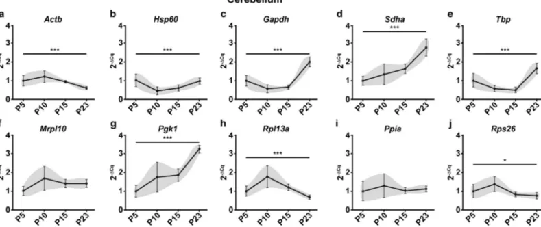
variation across experimental groups does not faithfully recapitulate the extent of variation in actual RNA quantities. Hence, we have represented this data as RNA fold changes (2-ΔCq) across time points.

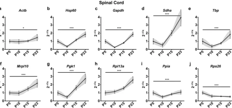
The first statistical test to assess stability after visually representing the data was One-way ANOVA to determine if the mean mRNA levels across groups are significantly different from one another. In the cerebellum, 8 of the 10 reference genes tested (Actb, Hsp60, Gapdh, Sdha, Tbp, Pgk1, Rpl13a and Rps26) showed significant variation in the mRNA levels across time

points (Fig 2) Only 2 genes (Mrpl10, Ppia) showed no significant change. In the spinal cord, all

tested genes showed significant variation in mRNA levels across the four time points (Fig 3). These results taken together with the raw expression profiles ofMbp (Fig 1B,Fig 1D) show that intrinsic changes in mRNA levels of reference genes can indeed skew the normalized pro-file ofMbp. As a result, it causes a significant bias in the results and interpretations that ensue

thus highlighting the importance of validating reference gene stability in longitudinal studies.

Assessment of expression stability using multiple statistical approaches

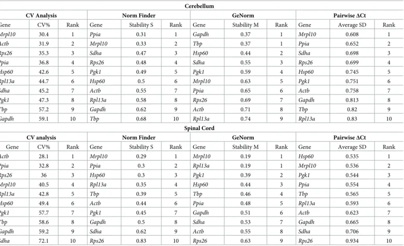
The expression stability of candidate reference genes was analyzed in both tissues using four well known statistical methods—CV analysis [20], NormFinder [19], GeNorm [18] and the PairwiseΔCt method [21] (Table 1).

CV analysis. The CV analysis estimates the variation in the linearized Cq values (2-Cq) of a reference gene across all samples taken together (S1 Table). CV for each gene is calculated as the ratio of the standard deviation to the mean and it is expressed as a percentage. A lower CV would therefore mean higher stability. CV analysis on the cerebellum samples revealed

Mrpl10, Actb and Rps26 as the top three stable reference genes. In the spinal cord, the top three

reference genes areActb, Ppia, Rps26.

Fig 2. Raw expression profiles of reference genes expressed as fold changes across experimental groups (2-ΔCq) at P5, 10, 15 and 23 in the cerebellum. P5 group is the experimental calibrator. (a) Actb, (b) Hsp60, (c) Gapdh, (d) Sdha, (e) Tbp, (f) Mrpl10, (g) Pgk1, (h) Rpl13a, (i) Ppia and (j) Rps26. Results are expressed as the Mean± SD for each time point. One-way ANOVA was performed to assess differences between the means of all groups. Statistical significance is denoted by ‘�_’

representing P values:�_P<0.05,��_P<0.01,���_{P<0.001. The grey area around each profile denotes the evolution of the intergroup and intragroup variation across time}

points.

NormFinder analysis. We next analyzed our data using NormFinder which uses a

model-based approach which calculates the stability of reference genes based on two parame-ters–the intergroup variation and the intragroup variation. The stability score denoted by the S value is a weighted measure of these two parameters. The most stable reference gene has the least S value. In the cerebellum, NormFinder identifiedPpia, Mrpl10 and Sdha as the top three

stable genes. In the spinal cord, the algorithm identifiedMrpl10, Ppia and Hsp60 as the top

three stable reference genes.

GeNorm analysis. GeNorm calculates stability based on pairwise variation. The rationale

is that if two genes vary similarly across all samples, then they are the most stable reference genes for that dataset. All other genes are ranked on their similarity to the expression of the top two genes. The algorithm functions by first identifying two genes with the highest expres-sion agreement and therefore high stability. It then calculates the expresexpres-sion variation of every other gene sequentially with respect to the previous genes chosen. Therefore, the ranking of the GeNorm algorithm always has 2 genes at the top with the same M value followed by other genes with higher M values indicating lower stability. In the cerebellum, the GeNorm algo-rithm identifiedGapdh and Tbp to be the most stable reference genes followed by Hsp60. This

is in stark contrast to the genes identified by the previous two methods. In the spinal cord, the most stable reference genes were identified asMrpl10 and Rpl13a followed by Pgk1.

PairwiseΔCt analysis. This method works on the same rationale as GeNorm but

calcu-lates the stability value (Mean SD) differently. It is calculated as the average standard deviation of the Cq value differences that the gene exhibits with other genes (S2 Table). In the cerebel-lum, pairwiseΔCt analysis identified Mrpl10, Ppia and Sdha as the top three most stable refer-ence genes. The ranking of this method and NormFinder are quite similar in the cerebellum. Fig 3. Raw expression profiles of reference genes expressed as fold changes across experimental groups (2-ΔCq) at P5, 10, 15 and 23 in the spinal cord. P5 group is the experimental calibrator. (a) Actb, (b) Hsp60, (c) Gapdh, (d) Sdha, (e) Tbp, (f) Mrpl10, (g) Pgk1, (h) Rpl13a, (i) Ppia and (j) Rps26. Results are expressed as the Mean± SD for each time point. One-way ANOVA was performed to assess differences between the means of all groups. Statistical significance is denoted by ‘�_’

representing P values:�_P<0.05,��_P<0.01,���_{P<0.001. The grey area around each profile denotes the evolution of the intergroup and intragroup variation across time}

points.

However, in the spinal cord the top three genes were identified asHsp60, Mrpl10 and Pgk1,

noticeably different from the NormFinder rankings.

The overall ranking of genes across all methods recapitulated inTable 1show that the sta-bility ranking of reference genes can indeed vary significantly depending on the tissue studied and the method used for validation. This makes the identification of the best reference genes very cumbersome.

Suitability of validation methods for longitudinal studies

We next analyzed the suitability of these methods in a longitudinal setting highlighting the assumptions of each method and the factors that influence the stability scores.

CV analysis. As mentioned, the CV analysis adopts a direct approach by calculating the

variance of a gene across all samples taken together. However, this method does not consider the variation across different time points or groups. For example,Actb is ranked 2ndin the cer-ebellum (Table 1) as it exhibits low overall variation but the profile of the gene (Fig 2A) tells us that it does vary across time points. This is a major concern in a longitudinal study as this method determines variation in just one dimension whereas the dataset exists in two dimensions.

NormFinder analysis. The NormFinder approach is more robust as it calculates the

sta-bility based on the intergroup and intragroup variation. However, on inspecting the algorithm Table 1. Expression stability of candidate reference genes in cerebellum and spinal cord evaluated using Coefficient of Variation (CV) Analysis, NormFinder, GeN-orm and the PairwiseΔCt method.

Cerebellum

CV Analysis Norm Finder GeNorm PairwiseΔCt

Gene CV% Rank Gene Stability S Rank Gene Stability M Rank Gene Average SD Rank

Mrpl10 30.4 1 Ppia 0.31 1 Gapdh 0.37 1 Mrpl10 0.608 1 Actb 31.9 2 Mrpl10 0.33 2 Tbp 0.37 1 Ppia 0.652 2 Rps26 35.3 3 Sdha 0.47 3 Hsp60 0.44 2 Sdha 0.698 3 Ppia 36.8 4 Rps26 0.48 4 Sdha 0.55 3 Rps26 0.699 4 Hsp60 42.6 5 Pgk1 0.49 5 Pgk1 0.59 4 Hsp60 0.745 5 Rpl13a 44.7 6 Hsp60 0.5 6 Mrpl10 0.63 5 Pgk1 0.751 6

Sdha 45.2 7 Actb 0.55 7 Ppia 0.65 6 Actb 0.758 7

Pgk1 47.3 8 Rpl13a 0.58 8 Rps26 0.69 7 Gapdh 0.813 8

Tbp 57.2 9 Gapdh 0.62 9 Actb 0.71 8 Tbp 0.82 9

Gapdh 59.1 10 Tbp 0.68 10 Rpl13a 0.74 9 Rpl13a 0.83 10

Spinal Cord

CV analysis Norm Finder GeNorm PairwiseΔCt

Gene CV% Rank Gene Stability S Rank Gene Stability M Rank Gene Average SD Rank

Actb 28.1 1 Mrpl10 0.29 1 Mrpl10 0.19 1 Hsp60 0.535 1

Ppia 32.8 2 Ppia 0.3 2 Rpl13a 0.19 1 Mrpl10 0.536 2

Rps26 36 3 Hsp60 0.3 3 Pgk1 0.39 2 Pgk1 0.544 3

Mrpl10 40.5 4 Rpl13a 0.35 4 Hsp60 0.44 3 Ppia 0.554 4

Rpl13a 42.8 5 Tbp 0.39 5 Tbp 0.46 4 Tbp 0.565 5

Hsp60 49.4 6 Actb 0.44 6 Ppia 0.48 5 Rpl13a 0.593 6

Pgk1 57.7 7 Pgk1 0.45 7 Gapdh 0.51 6 Actb 0.623 7

Tbp 58.6 8 Gapdh 0.5 8 Sdha 0.53 7 Gapdh 0.665 8

Gapdh 59.2 9 Sdha 0.62 9 Actb 0.55 8 Sdha 0.706 9

Sdha 72.1 10 Rps26 0.83 10 Rps26 0.63 9 Rps26 0.934 10

further, we found that including genes with high overall variation can affect the stability rank-ings of all the genes. Consider the overall variation ofActb in the spinal cord (Fig 3A). It has a CV of 28.1% (Table 1), which is the least among all genes in that group. Furthermore, the pro-file ofActb in the spinal cord is almost flat with minimal variation across groups (Fig 3A). Nev-ertheless, it is ranked 6thin the NormFinder method.Hsp60 and Rpl13a, on the other hand,

with a higher overall variance and significant intergroup variation when compared toActb

(Fig 3A,Fig 3BandFig 3H) are ranked 3rdand 4th.Hsp60 is in fact attributed the same stability

value asPpia which is ranked 2nd. This possible flaw in the algorithm is because of the presence of genes with high overall variations. Hence, the NormFinder algorithm can potentially be improved after identifying and removing genes with high overall variation(See Towards an integrated approach).

GeNorm analysis. The GeNorm algorithm as explained earlier ranks genes based on

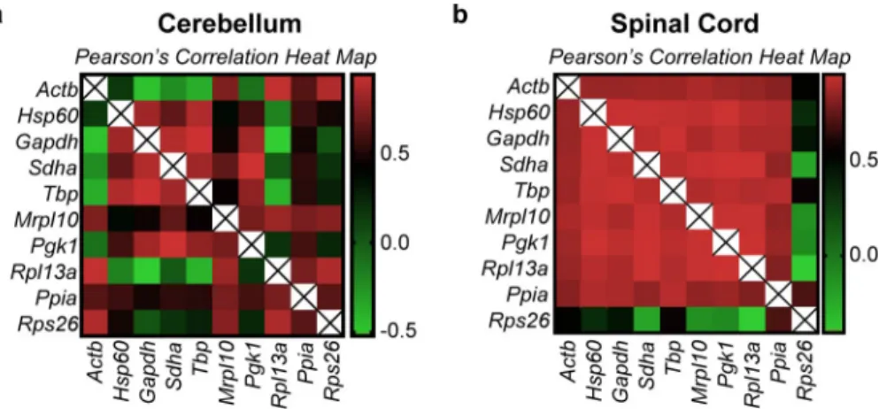
pair-wise correlation. Hence, there is a possibility that this method could estimate correlated and co-regulated genes to be highly stable. To validate the rankings of this algorithm we performed Pearson’s correlation on the linearized Cq values of all genes and samples (Fig 4,S3 Tableand S4 Table). We observed two distinct patterns of correlation in the cerebellum and the spinal cord, the cerebellum being more heterogeneous. In the spinal cord, almost all genes tested exhibit a positive correlation exceptActb which correlates less and Rps26 which exhibits

nega-tive correlation with most of the other genes. This is also evident from the raw expression pro-files where we see that the raw expression propro-files in the cerebellum are heterogeneous (Fig 2). In the spinal cord, however, all the reference genes seem to have a similar profile except for

Actb and Rps26 (Fig 3).

Interestingly, the highest correlation in the cerebellum dataset was observed inGapdh/Tbp

with a Pearson’s r score of 0.937. This gene pair is ranked first in the GeNorm analysis (Table 1) but have the highest overall variation in the group (CV = 59.1% and 57.2%). In the spinal cord, however, the top two genes according to GeNorm areMrpl10/Rpl13a while the

highest correlation is observed inSdha/Pgk1 with a Pearson’s r score of 0.97. Intriguingly, the

genes that are classed below—Pgk1, Hsp60 and Tbp have CV values of 57.8%, 49.4% and

58.6%, which are among the highest in the spinal cord group. This is because of their Fig 4. Pearson’s correlation heatmap of the linearized Cq values (2-Cq_{) of all genes. Pearson’s correlation of all}

genes was performed to identify the extent of expression correlation in (a) cerebellum and (b) spinal cord. The colour scheme is denoted next to each heatmap. The numerical values used in the colour scheme represent the Pearson’s r score. r = 0 (no correlation), r = +0.5 (positive correlation), r = -0.5 (negative correlation). r values closer to +1 or -1 denote strong positive and negative correlations respectively. The diagonal lines marked with an “X” are indicative of the correlation of a gene with itself and therefore is omitted from analysis.

expression agreement with the top two genes. Seemingly stable genes such asPpia

(CV = 32.8%,Fig 3I) andActb (CV = 28.1%,Fig 3A) are pushed to the lower half of the rank-ing (Table 1).

These results suggest that GeNorm tends to favor highly correlated genes in a heteroge-neously correlated set of genes (cerebellum dataset). In a less heterogenous dataset (spinal cord) the ranking does not concur with the overall stability of the genes across samples assessed by visual representation (Fig 3) and CV analysis (Table 1). These results taken together show that GeNorm’s ranking can be influenced by the extent of correlation in the dataset. This exclusion of possibly stable genes by GeNorm because of negative or less correla-tion was indeed foreseen by Anderson and colleagues when they proposed the NormFinder model. We find that to be true in our analysis.

PairwiseΔCt Analysis. The pairwise ΔCt approach seems to work better in a

heteroge-neously correlated set of genes. The rankings of NormFinder and the pairwiseΔCt methods are rather identical in the cerebellum. However, in the spinal cord apart fromMrpl10 the

other top genes—Pgk1 and Hsp60—show high variation across samples as explained earlier.

The limitations of this method can also be observed in the spinal cord.Actb, which shows a

rather flat profile (Fig 3A) is very distinct when compared to the others. It correlated very little with other genes (Fig 4BandS4 Table). This increases the difference in the Cq values betweenActb and others resulting in a high Mean SD (stability value) thereby attributing it

with a lower rank. Therefore, although a gene varies very little across samples and groups, the pairwiseΔCt approach might attribute it with a lower rank if the profiles of the other genes are different. The same argument is also true forRps26 in the spinal cord (Fig 3Jand Fig 4B)

In conclusion, we find that the ranking of all the methods except CV analysis is influenced by the inclusion of genes with high overall variation. Additionally, the pairwise expression sta-bility methods (GeNorm and PairwiseΔCt) could produce misleading results depending on the profile of the highly variable genes together with the extent of expression correlation between all the genes.

Towards an integrated approach

The first step towards an integrated approach was to remove genes with high overall variance. CV analysis calculates the overall variance of each gene and it is the only method where the sta-bility ranking of a gene is not influenced by others. We therefore used this method to objec-tively identify genes with high overall variance. We defined a threshold of CV = 50%. Genes that exhibit a CV above this value are taken to be highly variable and are excluded from further analysis. In the cerebellum,Gapdh and Tbp were removed and in the spinal cord Gapdh, Tbp, Pgk1 and Sdha were removed from analysis. We next determined how this exclusion impacts

the stability ranking of NormFinder, GeNorm and the PairwiseΔCt approach in both tissues (Table 2).

Ranking changes in NormFinder. As expected, exclusion of highly variable genes

changed the overall ranking of the NormFinder algorithm in the cerebellum (Table 2). Although the top two genes remained the same, the ranking of other genes changed.Sdha, Hsp60 and Pgk1 that were ranked higher than Actb (Table 1) now obtained ranks lower than

Actb (Table 2). The top three genes after exclusion ofGapdh and Tbp were identified as Mrpl10, Ppia and the third position is shared between Rps26 and Actb. The most stable genes

identified by NormFinder after exclusion (Table 2) concurs with the CV analysis (Table 1) and with the expression profiles of the genes (Fig 2A,Fig 2F,Fig 2IandFig 2J) wherein the most stable genes exhibit minimal variation across time points.

In the spinal cord, similar changes were observed.Ppia was now ranked above Mrpl10 and

these two were identified as the top two (Table 2). However, the third rank was now attributed toActb. Hsp60, which was previously third finds itself in the lower half of the ranking. Again,

the top three genes identified exhibit low overall variation in the spinal cord and their profiles exhibit minimal variation across timepoints (Fig 3A,Fig 3FandFig 3I).

This indeed shows that exclusion of highly variable genes potentially improves the perfor-mance of the NormFinder method and can help in improving the quality of the results.

Ranking changes in GeNorm. The changes observed in GeNorm were more drastic in

the cerebellum. The new rankings were almost the inverse of the previous rankings (Tables1 and2) withActb/Rpl13a now identified as the most stable genes followed by Rps26, Mrpl10

andPpia. These results, although astonishing, made sense when interpreted with the raw

expression profiles (Fig 2). In the absence ofGapdh and Tbp, the algorithm has chosen Actb/ Rpl13a to be the most stable. Notice how the profiles of these two genes are very similar (Fig 2AandFig 2H). The genes ranked just below also have as similar profile to these two. In effect, the previous GeNorm rankings (Table 1) were based on genes that had profiles similar to

Gapdh/Tbp (U shaped curve) whereas the new rankings are based on genes with the exact

inverted profile exhibited byActb and Rpl13a. This change in ranking brings to evidence the

possible biases that can occur when using GeNorm in a heterogeneously correlated data set. In the spinal cord, however, the changes were not so drastic. The top two genesMrpl10/ Rpl13a remained the same (Tables1and2). Nevertheless, the genes that were ranked below showed some noticeable change.Actb and Ppia are now ranked above Hsp60. In the spinal

cord, most of the genes are correlated (Fig 4B) and their profiles look alike exceptRps26 (Fig 3J). Therefore, the top two genes did not change even after the exclusion of the highly variable genes. However, in the absence of these genes, the profile ofActb (Fig 3A) now looks more like

Hsp60 0.64 8 Hsp60 0.67 7 Hsp60 0.823 8

Spinal Cord

Norm Finder GeNorm PairwiseΔCt

Gene Stability S Rank Gene Stability M Rank Gene Average SD Rank

Ppia 0.22 1 Mrpl10 0.19 1 Mrpl10 0.472 1

Mrpl10 0.25 2 Rpl13a 0.19 1 Ppia 0.49 2

Actb 0.28 3 Actb 0.32 2 Actb 0.494 3

Rpl13a 0.35 4 Ppia 0.39 3 Rpl13a 0.537 4

Hsp60 0.48 5 Hsp60 0.47 4 Hsp60 0.68 5

Rps26 0.64 6 Rps26 0.58 5 Rps26 0.78 6

In the cerebellum, Gapdh and Tbp were excluded from analysis. In the spinal cord, 4 genes–Sdha, Gapdh, Tbp and Pgk1 were excluded from analysis

Mrpl10/Rpl13a than Ppia or Hsp60 (Fig 3B,Fig 3F,Fig 3HandFig 3I). This is a possible reason for the change in ranks observed.

These results taken together yet again show that GeNorm results can prove to be highly biased depending on the correlation observed in the dataset and the expression agreement between candidate genes.

Ranking changes in Pairwise

ΔCt method

In the cerebellum, the changes observed are very similar to the changes observed in the Norm-Finder algorithm (Table 2).Mrpl10 and Ppia are still ranked as the top two. However, Actb

andRpl13a are now ranked above Sdha, Pgk1 and Hsp60. Indeed, the removal of Gapdh and Tbp decreased the difference in Cq values between Actb and other genes thereby leading to

lower Mean SD (higher ranks). The same is true forRpl13a. Similarly, genes that resembled Gapdh and Tbp were now pushed to the bottom as their profiles look much different from the

top ranked reference genes. In other words, the difference between their Cq values and the others have increased across all samples. Interestingly, the ranking of the PairwiseΔCt method and NormFinder seem to concur a lot both before and after exclusion of highly variable genes (Tables1and2).

However, in the spinal cord, which shows high extent of homogenous correlation, the changes are rather significant. The top two genes now areMrpl10 and Ppia. This is followed by Actb. Hsp60 which was ranked 1stbefore exclusion (Table 1) is now close to the bottom of the ranking along withRps26 (Table 2). The reason for this change is the same as stated for the cer-ebellum. Removal of genes with high overall variation results in genes that had a similar profile to the genes removed being classed lower. However, this also depends on the similarity of the rest of the genes with the profile of the new highly ranked genes. This is a significant hurdle as the ranking of genes becomes inter dependent even after the removal of highly variable genes. In the spinal cord, the ranking of this method after exclusion concurs with NormFinder (Table 2), that was previously not the case (Table 1).

Discussion

As each method analyzed in the study has its own advantages and drawbacks, using any of these methods alone would not be enough to have bias-free results. Neither would averaging the ranks of genes determined from all these methods. Hence, there is a need to devise an inte-grated approach that is based on the suitability of the method in a longitudinal setting.

Among the different methods tested in this developmental study, we find that the methods that rely on pairwise variation (GeNorm and PairwiseΔCt method) are ill suited for reference gene validation. However, it should be noted that the predictions of the PairwiseΔCt method did improve after the exclusion of highly variable genes. Nevertheless, the ranking inter-dependency does pose a major problem for a longitudinal study.

Regarding the other two methods, the major drawback of the CV analysis is that it does not factor in the variation between groups but can however determine the absolute overall varia-tion. The major drawback of the NormFinder method is that the stability ranking of the method is influenced by genes with high overall variation. It can however calculate stability based on both intergroup and intragroup variation. Hence, using these two methods in tan-dem would negate their respective drawbacks. It goes without saying that visual representation of the raw expression profiles is also an additional tool that can be used to validate the findings of these two methods.

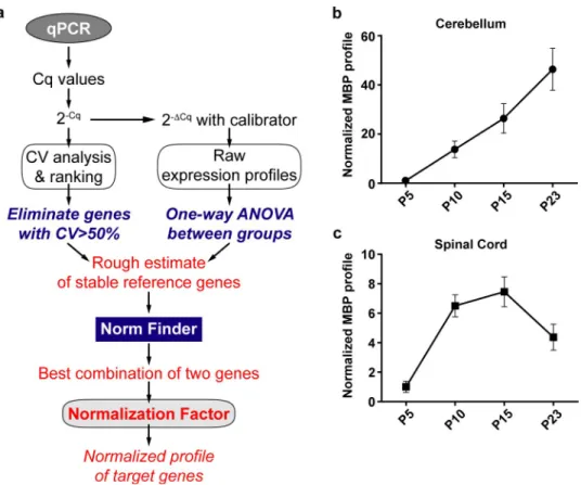
Taking all these factors into account, we propose an integrated approach that uses CV anal-ysis, visual representation (with ANOVA) and NormFinder to assess the best set of reference

genes for a longitudinal study (Fig 5). This method also recapitulates the method used in this study.

Once the Cq values of all samples and genes are obtained from qPCR, they are linearized, and CV analysis is performed. Parallelly, using the experimental calibrator, the raw experimen-tal profiles of all candidate genes are plotted as fold changes (2-ΔCq). This is followed by One-way ANOVA to assess the variation among all groups. It should be noted that ANOVA is used just to assess if there is significant statistical variation among the means of the groups. It does not assess, by any means, the extent of this variation. Thus, visual representation along with the results of CV analysis and ANOVA can help us obtain a rough estimate of the most stable reference genes. At this stage, genes that exhibit CV>50% are removed. The rest of the genes are then subjected to the NormFinder algorithm. The algorithm then ranks the genes based on intergroup and intragroup variation. It also detects the best two genes that can be used for nor-malization with a grouped stability value. These two genes are then used to calculate a normal-izing factor to normalize all target genes.

In our study, the integrated approach detectedMrpl10 and Ppia as the two best genes in

both tissues with a grouped stability of S = 0.17 in the cerebellum and S = 0.11 in the spinal cord. Nevertheless, we cannot be sure if the same genes would be the best references if another time point was added or if one of the time points studied here is removed. This limitation indeed exists for all reference gene validation studies. In other words, the best reference gene (s) identified by any study using any method is only suitable for that experimental setting and cannot be extrapolated.

Fig 5. Integrated approach to determine the best reference genes in a longitudinal study. (a) Proposed qPCR Workflow (b) Normalized Mbp expression profile in the cerebellum using Ppia and Mrpl10. (c) Normalized Mbp expression profile in the spinal cord using Ppia and Mrpl10.

Apart from the parameters that have been identified in this study that contribute to the suit-ability of a method, certain other factors are to be considered while constructing a validation study. Indeed, simple factors such as the total sample size and number of candidate reference genes play an important role on the suitability of a statistical method [22]. Similar issues have been detailed and standard guidelines have been established to facilitate standardization and reproducibility of qPCR assays [23].

A notable limitation of this study is the choice of the candidate reference genes. The candi-dates were chosen as they have been conventionally used for normalization of differential expression in the Central Nervous System. This means that we could have potentially excluded unknown and undiscovered stable references. A more thorough approach would be to choose candidate genes from high-throughput data to avoid this inherent bias [24–26].

In this study we analyzed four commonly used statistical methods. Indeed, other methods have been proposed to validate reference genes. Notably, the RefFinder [10] and the Best-Keeper [27] algorithms have been used commonly in a multitude of studies that validate refer-ence genes. Although we have not used them in our study, we have identified some key issues in their approaches. The RefFinder is a combinatory method that takes into consideration the stability rankings of GeNorm, NormFinder, BestKeeper and the PairwiseΔCt method. Depending on the rankings of the candidate genes across these different algorithms, it attri-butes an ordinal “weight” for each candidate gene. The final rankings are then computed as the geometric mean of the weighted rankings. We emphasize that such an approach is not sci-entifically sound as it does not consider the merits and demerits of these algorithms in a longi-tudinal setting. We therefore find that the rankings of the RefFinder tool is merely arithmetic in nature and has no intrinsic scientific rigor or validity. This observation has also been pointed out previously by De Spiegelaere and colleagues in their study [22].

The BestKeeper algorithm assesses stability based on Pearson’s correlation of candidate gene Cq values with the BestKeeper Index. Firstly, the algorithm eliminates genes that it con-siders highly variable by calculating the Standard Deviation of candidate gene Cq values across all samples. The authors define a threshold of SD = 1 cycle (RNA quantity difference by a fac-tor of 2). Any gene that exhibits SD>1 is deemed highly variable and removed from further analysis.

We remark that this threshold of SD = 1 is too lenient as it is calculated using just the Cq values where the actual fold changes in RNA quantities are underestimated. From our data (S5 Table), we find that genes that exhibit SD<1 (below BestKeeper Threshold) in Cq values can exhibit CV values (of 2-Cq) well above 50% which we believe is indicative of high variation in RNA fold changes. In turn, this elimination process based solely on variation in Cq values can decrease the robustness of the algorithm as it is dependent on the elimination of highly vari-able genes. We have also observed using our data that the Pearson’s correlation analysis (the core of the BestKeeper algorithm) of Cq values are largely different from the correlation analy-sis of 2-Cqvalues with significant differences in Pearson’s r score. As minor changes in Cq val-ues can imply huge changes in RNA quantities, correlation analysis of Cq valval-ues would produce a biased assessment of the actual correlation present in RNA quantities. We thus believe that this algorithm can potentially be improved by taking these factors into consideration.

Finally, the integrated approach proposed in this study is only applicable for a longitudinal setting. How these methods fare in cross sectional studies remains to be explored. However, the approach proposed in this study addresses an important observation that has been con-stantly made but systematically overlooked in validation studies. Our integrated approach, in effect, is contradictory to previously held notions that all statistical approaches are applicable to any experimental setting and that a minimum of three different statistical approaches are

Spinal Cord (P5: N = 6, P10: N = 5, P15: N = 7, P23: N = 6) Total number of samples = 24 All aspects of animal care and animal experimentation were performed in accordance with the relevant guidelines and regulations of INSERM, Universite´ Paris Descartes and approved by the French National Committee of Animal experimentation and ethics (Ref n˚:

2016092216181520).

Total RNA isolation

Tissues were dissected out from mice at the stipulated time points, immediately frozen in liquid nitrogen and stored at -80˚C. Samples were later thawed in 1mL of TRIzol reagent (Ambion Life Technologies 15596018) on ice followed by homogenization in a bead mill homogenizer (RETSCH MM300) with 5mm RNase free stainless-steel beads. Homogenization was carried out for 4 minutes at 20Hz (2 x 2 minutes) with a 3-minute pause in between when the samples were placed on ice to cool down. Next, RNA was extracted from the homogenate using the manufacturer’s instructions with slight modifications. Briefly, 100% Ethanol was substituted for Isopropanol to reduce the precipitation of salts. Also, RNA precipitation was carried out over-night at -20˚C in the presence of glycogen. The following day, precipitated RNA was pelleted by centrifugation and washed at least 3 times with 70% Ethanol to eliminate any residual contami-nation. Tubes were then spin dried in vacuum for 10 minutes and RNA was resuspended in 30μL of RNase Free water (Ambion AM9937). RNA was then stored at -80˚C till RT-PCR.

RNA quality, integrity and assay

RNA quantity was assayed using UV spectrophotometry on Nanodrop One (Thermo Scien-tific). Optical density absorption ratios A260/A280 & A260/A230 of the cerebellum samples were 1.86(±0.03 SD) and 2.29 (±0.07 SD) respectively. The corresponding values for the spinal cord samples were 1.95 (±0.03 SD) and 2.08 (±0.32 SD) respectively. Furthermore, RNA integ-rity was verified using denaturing formaldehyde agarose gel electrophoresis. All samples showed intact bands for 28S and 18S rRNA and were subsequently used for RTqPCR.

RTqPCR

500ng of Total RNA was first subjected to DNase digestion (Promega M6101) at 37˚C for 30 minutes to eliminate contaminating genomic DNA. Next, DNase activity was stopped using DNase Stop Solution (Promega M199A) and RNA was reverse transcribed with Random Primers (Promega C1181) and MMLV Reverse Transcriptase (Sigma M1302) according to prescribed protocols. Quantitative Real time PCR (qPCR) was performed using Takyon ROX SYBR 2X MasterMix (Eurogentec UF-RSMT-B0701) as a fluorescent detection dye. All reac-tions were carried out in a final volume of 7μl in 384 well plates with 300 nM gene specific primers, around 7ng of cDNA (at 100% RT efficiency) and 1X SYBR Master Mix in each well.

Each reaction was performed in triplicates. All qPCR experiments were performed on BioRad CFX384.

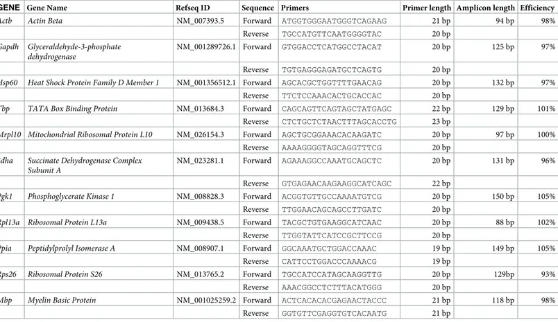
Primer design

All primers used in the study were designed using the Primer 3 plus software (https:// primer3plus.com/cgi-bin/dev/primer3plus.cgi). Splice variants and the protein coding sequence of the genes were identified using the Ensembl database (www.ensembl.org). Consti-tutively expressed exons among all splice variants were then identified using the ExonMine database (www.imm.fm.ul.pt/exonmine/). Primer sequences that generated amplicons span-ning two constitutively expressed exons were then designed using the Primer 3 plus software. For detailed information on Primer sequences refer toTable 3.

Amplification efficiencies

The amplification efficiencies of primers were calculated using serial dilution of cDNA mole-cules. Briefly, cDNA preparations from Cerebella and Spinal cords from different age groups of mice were pooled and serially diluted three times by a factor of 10. qPCR was then per-formed using these dilutions and the results were plotted as a standard curve against the respective concentration of cDNA. Amplification efficiency (E) was calculated by linear regres-sion of standard curves using the following equation

E ¼ 10 ðslope of the standard curve1 Þ

Table 3. Details of the primer sequences used in the study.

GENE Gene Name Refseq ID Sequence Primers Primer length Amplicon length Efficiency

Actb Actin Beta NM_007393.5 Forward ATGGTGGGAATGGGTCAGAAG 21 bp 94 bp 98%

Reverse TGCCATGTTCAATGGGGTAC 20 bp

Gapdh Glyceraldehyde-3-phosphate dehydrogenase

NM_001289726.1 Forward GTGGACCTCATGGCCTACAT 20 bp 125 bp 97%

Reverse TGTGAGGGAGATGCTCAGTG 20 bp

Hsp60 Heat Shock Protein Family D Member 1 NM_001356512.1 Forward AGCACGCTGGTTTTGAACAG 20 bp 132 bp 97%

Reverse TTCTCCAAACACTGCACCAC 20 bp

Tbp TATA Box Binding Protein NM_013684.3 Forward CAGCAGTTCAGTAGCTATGAGC 22 bp 129 bp 101%

Reverse CTCTGCTCTAACTTTAGCACCTG 23 bp

Mrpl10 Mitochondrial Ribosomal Protein L10 NM_026154.3 Forward AGCTGCGGAAACACAAGATC 20 bp 97 bp 100%

Reverse AAAAGGGGTAGCAGGTTTCG 20 bp

Sdha Succinate Dehydrogenase Complex Subunit A

NM_023281.1 Forward AGAAAGGCCAAATGCAGCTC 20 bp 131 bp 96%

Reverse GTGAGAACAAGAAGGCATCAGC 22 bp

Pgk1 Phosphoglycerate Kinase 1 NM_008828.3 Forward ACGGTGTTGCCAAAATGTCG 20 bp 150 bp 105%

Reverse TTGGAACAGCAGCCTTGATC 20 bp

Rpl13a Ribosomal Protein L13a NM_009438.5 Forward TACGCTGTGAAGGCATCAAC 20 bp 88 bp 102%

Reverse TTGGTATTCATCCGCTTCCG 20 bp

Ppia Peptidylprolyl Isomerase A NM_008907.1 Forward GGCAAATGCTGGACCAAAC 19 bp 149 bp 105%

Reverse CATTCCTGGACCCAAAACG 19 bp

Rps26 Ribosomal Protein S26 NM_013765.2 Forward TGCCATCCATAGCAAGGTTG 20 bp 129bp 93%

Reverse AAACGGCCTCTTTACATGGG 20 bp

Mbp Myelin Basic Protein NM_001025259.2 Forward ACTCACACACGAGAACTACCC 21 bp 118 bp 98%

cases, one outlier Cq was removed so as to have at least duplicate Cq values for each biological sample and an SD<0.25.

Statistical analysis

Statistical analysis for reference gene validation was performed using R software packages and Microsoft Excel. GeNorm [18] analysis was performed using the ReadqPCR and NormqPCR packages in R[29]. Normfinder [19] analysis was performed using NormFinder for R (https:// moma.dk). Co-efficient of Variance Analysis was performed in Microsoft Excel. The Cq values were first transformed to a linear scale (linearization) by calculating 2-Cqfor each sample. CV analysis was then performed on 2-Cqvalues (S1 Table). PairwiseΔCt analysis was also per-formed in Microsoft Excel (S2 Table).

To assess statistical difference in RNA quantities between groups, One-way ANOVA was performed in Graph Pad Prism v7.0. Pearson’s correlation matrix of reference genes and the heat maps were also generated in Graph Pad Prism v7.0.

The normalization factor was determined by first calculating the arithmetic mean of the Cq values from the 2 best genes determined by the workflow. The mean Cq values were linearized and then used to normalize target genes using the 2-ΔΔCtmethod [30,31]. The P5 group was used as the experimental calibrator. Data was visualized using Graph Pad Prism v7.0.

Supporting information

S1 Table. CV analysis example. The Cq values of all samples are linearized. The CV is then

calculated as the ratio of the SD to the mean of the linearized Cq values. It is expressed as a per-centage. A lower CV value would mean lower variation across samples and therefore higher stability.

(DOCX)

S2 Table. PairwiseΔCt analysis example. The table shows the stability calculation by the

Pair-wiseΔCt method for Actb. It is a table of Cq value differences between Actb and all the other genes. Each row represents a sample and each column represents a gene. The difference in Cq values betweenActb and the others is first calculated across all samples. Therefore, the first

col-umn has 0s (difference in Cq ofActb with itself) Next, the standard deviation of the differences

is calculated at the end of each column indicated by SD. The stability value (Average SD) of

Actb is then calculated as the arithmetic mean of these standard deviations.

(DOCX)

S3 Table. Pearson’s correlation matrix for the cerebellum.

S4 Table. Pearson’s correlation matrix for the spinal cord.

(DOCX)

S5 Table. Raw qPCR output data.

(XLSX)

Acknowledgments

The authors did not receive any specific funding for this study. The authors would like to thank Paris Descartes University and INSERM. V.K.S. and N.K.S. received their PhD fellow-ships from the French Ministry of Research and Innovation. The authors would like to acknowledge Ce´line Becker and Claire Mader (Saints-Pères Animal Facility) for the breeding and management of the animals used in the study.

Author Contributions

Conceptualization: Venkat Krishnan Sundaram, Nirmal Kumar Sampathkumar. Formal analysis: Venkat Krishnan Sundaram, Nirmal Kumar Sampathkumar. Investigation: Venkat Krishnan Sundaram, Nirmal Kumar Sampathkumar. Methodology: Venkat Krishnan Sundaram.

Validation: Charbel Massaad, Julien Grenier. Visualization: Julien Grenier.

Writing – original draft: Venkat Krishnan Sundaram.

Writing – review & editing: Nirmal Kumar Sampathkumar, Charbel Massaad, Julien Grenier.

References

1. Bustin SA. Absolute quantification of mRNA using real-time reverse transcription polymerase chain reaction assays [Internet]. Journal of Molecular Endocrinology. 2000. Available:http://www. endocrinology.org

2. Thellin O, Zorzi W, Lakaye B, De Borman B, Coumans B, Hennen G, et al. Housekeeping genes as internal standards: use and limits [Internet]. Journal of Biotechnology. 1999. Available:www.elsevier. com/locate/jbiotec

3. Kozera B, Rapacz M. Reference genes in real-time PCR. J Appl Genet. Springer Berlin Heidelberg; 2013; 54: 391–406.https://doi.org/10.1007/s13353-013-0173-xPMID:24078518

4. Dheda K, Huggett JF, Chang JS, Kim LU, Bustin SA, Johnson MA, et al. The implications of using an inappropriate reference gene for real-time reverse transcription PCR data normalization. Anal Biochem. Academic Press; 2005; 344: 141–143.https://doi.org/10.1016/J.AB.2005.05.022PMID:16054107

5. Lee JM, Roche JR, Donaghy DJ, Thrush A, Sathish P. Validation of reference genes for quantitative RT-PCR studies of gene expression in perennial ryegrass (Lolium perenne L.). BMC Mol Biol. BioMed Central; 2010; 11: 8.https://doi.org/10.1186/1471-2199-11-8PMID:20089196

6. Langnaese K, John R, Schweizer H, Ebmeyer U, Keilhoff G. Selection of reference genes for quantita-tive real-time PCR in a rat asphyxial cardiac arrest model. BMC Mol Biol. BioMed Central; 2008; 9: 53.

https://doi.org/10.1186/1471-2199-9-53PMID:18505597

7. Spinsanti G, Panti C, Bucalossi D, Marsili L, Casini S, Frati F, et al. Selection of reliable reference genes for qRT-PCR studies on cetacean fibroblast cultures exposed to OCs, PBDEs, and 17β-estradiol. Aquat Toxicol. Elsevier; 2008; 87: 178–186.https://doi.org/10.1016/J.AQUATOX.2008.01.018PMID:

18339435

8. Cheung TT, Weston MK, Wilson MJ. Selection and evaluation of reference genes for analysis of mouse (Mus musculus) sex-dimorphic brain development. PeerJ. PeerJ, Inc; 2017; 5: e2909.https://doi.org/ 10.7717/peerj.2909PMID:28133578

for RT-qPCR studies in neurodegenerative diseases. Sci Rep. Nature Publishing Group; 2016; 6: 37116.https://doi.org/10.1038/srep37116PMID:27853238

14. Mallona I, Lischewski S, Weiss J, Hause B, Egea-Cortines M. Validation of reference genes for quanti-tative real-time PCR during leaf and flower development in Petunia hybrida. BMC Plant Biol. BioMed Central; 2010; 10: 4.https://doi.org/10.1186/1471-2229-10-4PMID:20056000

15. Fu Y, Ruszna´ k Z, Herculano-Houzel S, Watson C, Paxinos G. Cellular composition characterizing post-natal development and maturation of the mouse brain and spinal cord. Brain Struct Funct. Springer Ber-lin Heidelberg; 2013; 218: 1337–1354.https://doi.org/10.1007/s00429-012-0462-xPMID:23052551

16. Hughes EG, Appel B. The cell biology of CNS myelination. Curr Opin Neurobiol. 2016; 39: 93–100.

https://doi.org/10.1016/j.conb.2016.04.013PMID:27152449

17. Bercury KK, Macklin WB. Dynamics and mechanisms of CNS myelination. Dev Cell. Elsevier; 2015; 32: 447–58.https://doi.org/10.1016/j.devcel.2015.01.016PMID:25710531

18. Vandesompele J, De Preter K, Pattyn F, Poppe B, Van Roy N, De Paepe A, et al. Accurate normaliza-tion of real-time quantitative RT-PCR data by geometric averaging of multiple internal control genes. Genome Biol. 2002; 3: RESEARCH0034.https://doi.org/10.1186/gb-2002-3-7-research0034PMID:

12184808

19. Andersen C, Jensen J, Orntoft T. Normalization of Real Time Quantitative Reverse Transcription -PCR Data: A Model - Based Variance Estimation Approach to Identify Genes Suited for Normalization, Applied to Bladder and Colon Cancer Data Sets. Cancer Res. 2004; 64: 5245.https://doi.org/10.1158/ 0008-5472.CAN-04-0496PMID:15289330

20. Boda E, Pini A, Hoxha E, Parolisi R, Tempia F. Selection of Reference Genes for Quantitative Real-time RT-PCR Studies in Mouse Brain. J Mol Neurosci. Humana Press Inc; 2009; 37: 238–253.https:// doi.org/10.1007/s12031-008-9128-9PMID:18607772

21. Silver N, Best S, Jiang J, Thein SL. BMC Molecular Biology Selection of housekeeping genes for gene expression studies in human reticulocytes using real-time PCR. 2006; https://doi.org/10.1186/1471-2199-7-33

22. De Spiegelaere W, Dern-Wieloch J, Weigel R, Schumacher V, Schorle H, Nettersheim D, et al. Refer-ence gene validation for RT-qPCR, a note on different available software packages. PLoS One. 2015; 10: 1–13.https://doi.org/10.1371/journal.pone.0122515PMID:25825906

23. Bustin SA, Benes V, Garson JA, Hellemans J, Huggett J, Kubista M, et al. The MIQE Guidelines: Mini-mum Information for Publication of Quantitative Real-Time PCR Experiments. 2009;https://doi.org/10. 1373/clinchem.2008.112797PMID:19246619

24. Eisenberg E, Levanon EY. Human housekeeping genes, revisited. Trends Genet. Elsevier; 2013; 29: 569–74.https://doi.org/10.1016/j.tig.2013.05.010PMID:23810203

25. Hoang VLT, Tom LN, Quek X-C, Tan J-M, Payne EJ, Lin LL, et al. RNA-seq reveals more consistent ref-erence genes for gene expression studies in human non-melanoma skin cancers. PeerJ. PeerJ, Inc; 2017; 5: e3631.https://doi.org/10.7717/peerj.3631PMID:28852586

26. Zhou Z, Cong P, Tian Y, Zhu Y. Using RNA-seq data to select reference genes for normalizing gene expression in apple roots.https://doi.org/10.1371/journal.pone.0185288PMID:28934340

27. Pfaffl MW, Tichopad A, Prgomet C, Neuvians TP. Determination of stable housekeeping genes, differ-entially regulated target genes and sample integrity: BestKeeper—Excel-based tool using pair-wise cor-relations. Biotechnol Lett. 2004; 26: 509–15. Available:http://www.ncbi.nlm.nih.gov/pubmed/15127793

PMID:15127793

28. Jacob F, Guertler R, Naim S, Nixdorf S, Fedier A, Hacker NF, et al. Careful Selection of Reference Genes Is Required for Reliable Performance of RT-qPCR in Human Normal and Cancer Cell Lines.

Huang S, editor. PLoS One. Public Library of Science; 2013; 8: e59180.https://doi.org/10.1371/journal. pone.0059180PMID:23554992

29. Perkins JR, Dawes JM, McMahon SB, Bennett DLH, Orengo C, Kohl M. ReadqPCR and NormqPCR: R packages for the reading, quality checking and normalisation of RT-qPCR quantification cycle (Cq) data. BMC Genomics. 2012; 13.https://doi.org/10.1186/1471-2164-13-296PMID:22748112

30. Schmittgen TD, Livak KJ. Analyzing real-time PCR data by the comparative C(T) method. Nat Protoc. 2008; 3: 1101–8. Available:http://www.ncbi.nlm.nih.gov/pubmed/18546601PMID:18546601

31. Livak KJ, Schmittgen TD. Analysis of relative gene expression data using real-time quantitative PCR and the 2^-ΔΔCT Method. Methods. 2001; 25: 402–408.https://doi.org/10.1006/meth.2001.1262