PlantGL: A Python-based geometric library for 3D plant modelling at different scales

HAL Id: hal-00850782

https://hal.inria.fr/hal-00850782

HAL is a multi-disciplinary open access

archive for the deposit and dissemination of sci-entific research documents, whether they are pub-lished or not. The documents may come from

L’archive ouverte pluridisciplinaire HAL, est destinée au dépôt et à la diffusion de documents scientifiques de niveau recherche, publiés ou non, émanant des établissements d’enseignement et de

PlantGL: A Python-based geometric library for 3D

plant modelling at different scales

Christophe Pradal, Frédéric Boudon, Christophe Nouguier, Jérôme Chopard,

Christophe Godin

To cite this version:

Christophe Pradal, Frédéric Boudon, Christophe Nouguier, Jérôme Chopard, Christophe Godin. PlantGL: A Python-based geometric library for 3D plant modelling at different scales. Graphical Models, Elsevier, 2009, 71 (1), 1–21, posted-at = 2008-11-04 14:10:07. �10.1016/j.gmod.2008.10.001�. �hal-00850782�

PlantGL: a Python-based geometric library

for 3D plant modelling at different scales

C. Pradal

, F. Boudon

∗

, C. Nouguier

, J. Chopard

,

C. Godin

a_{CIRAD, Virtual Plants INRIA Project-Team, UMR DAP, Montpellier, F-34398} France.

b_{INRIA, Virtual Plants INRIA Project-Team, UMR DAP, Montpellier, F-34398} France.

Abstract

In this paper, we present PlantGL, an open-source graphic toolkit for the creation, simulation and analysis of 3D virtual plants. This C++ geometric library is embedded in the Python language which makes it a powerful user-interactive platform for plant modeling in various biological application domains.

PlantGL makes it possible to build and manipulate geometric models of plants or plant parts, ranging from tissues and organs to plant populations. Based on a scene graph augmented with primitives dedicated to plant representation, several methods are provided to create plant architectures from either field measurements or procedural algorithms. Because they are particularly useful in plant design and analysis, special attention has been paid to the definition and use of branching system envelopes. Several examples from different modelling applications illustrate how PlantGL can be used to construct, analyse or manipulate geometric models at different scales ranging from tissues to plant communities.

Key words: Graphic library, Virtual plants, Crown envelopes, Plant architecture, Canopy reconstruction, Plant scene-graphs

1 _{These two authors contributed equally to the paper} ∗ Corresponding author.

1 Introduction

The representation of plant forms in computer scenes has long been recog-nized as a difficult problem in computer graphics applications. In the last two decades, several algorithms and software platforms have been proposed to solve this problem with a continuously improving level of efficiency, e.g. [1–9]. Due to the increasing use of computer models in biological research, the design of 3D geometric models of plants has also become an important aspect of var-ious biological applications in plant science, e.g. [10–16]. These applications raise specific problems that derive from the need to represent plants with a botanical or geometric accuracy at different scales, from tissues to plant com-munities. However, in comparison with computer graphics applications, less effort has been devoted to the development of geometric modelling systems adapted to the requirements of biological applications.

In this context, the most successful and widespread plant modelling system has been developed by P. Prusinkiewicz and his team since the late 80’s at the interface between biology and computer graphics. They designed a computer platform, known as L-Studio/VLab, for the simulation of plant growth based on L-systems [17,1,3]. This system makes it possible to model the develop-ment of plants with efficiency and flexibility as a process of bracketed-string rewriting. In a recent version of LStudio/VLab, Karwowski and Prusinkiewicz changed the original cpfg language for a compiled language, L+C, built on the top of the C++ programming language. The resulting gain of expressive-ness facilitates the specification of complex plant models in L+C [19]. An alternative implementation of a L-system-based software for plant modeling was designed by W. Kurth [20] in the context of forestry applications. This simulation system, called GroGra, was also recently re-engineered in order to model the development of objects more complex than bracketed strings. The resulting simulation system, GroIMP, is an open-source software that extends the chain rewriting principle of L-Systems to general graph rewriting with relational graph growth (RGG), [21,22]. Similarly to L+C, this system has been defined on top of a widely used programming language (here Java). Non-language oriented platforms were also developed. One of the first ones was designed by the AMAP group. The AMAP software [2,23] makes it possible to build plants by tuning the parameters of a predefined, hard-coded, model. Ge-ometric symbols for flowers, leaves, fruits, etc., are defined in a symbol library and can be modified or created with specific editors developed by AMAP. In this framework, a wide set of parameter-files has been designed corresponding to various plant species. In the context of applications more oriented toward computer graphics, the XFrog software [5,24] is a popular example of a plant simulation system dedicated to the intuitive design of plant geometric mod-els. In XFrog, components representing basic plant organs like leaves, spines, flowerlets or branches can be multiplied in space using high-level multiplier

components. Plants are thus defined as graphs representing series of multipli-cation operations. The XFrog system provides an easy to use, intuitive system to design plant models, with little biological expertise needed.

Therefore, if accuracy, conciseness and transparency of the modeling process is required, object-oriented, rule-based platforms, such as L-studio/VLab or GroIMP, are good candidates for modelers. If interactive and intuitive model design is required, with little biological expertise, then component-based sys-tems, like XFrog, or sketch-based systems are the best candidates. However, if easiness to explore and mathematically analyse plant scenes is required, none of the above approaches is completely satisfactory. Such an operation requires high-level user interaction with plant scenes and dedicated high-level mathematical primitives. With this aim, our team developed the AMAPmod software [25] several years ago, and its most recent version, VPlants, which enables modelers to create, explore and analyse plant architecture databases using a powerful script language. In a way complementary to L-Studio/VLab, VPlantsallows the user to efficiently analyse plant architecture databases and scenes from many exploratory perspectives in a language-based, interactive, manner [26–29]. The PlantGL library was developed to support geometric processing of plant scenes in VPlants, for applications ranging from computer graphics [30,31] to different areas of biological modeling [32–34,15,35,36]. A number of high-level requirements were imposed by this context. Similarly to AMAPmod/VPlants, the library should be open-source, it should be fully com-patible with the data structure used in AMAPmod/VPlants to represent plants, i.e.multi-scale tree graphs (MTGs), it should be accessible through an efficient script language to favor interactive exploration of plant databases, it should be easy to use for biologists or modellers and should not impose a particu-lar modelling approach, it should be easily extended by users to progressively adapt to the great variety of plant modelling applications, and finally, it should be interoperable with other main plant modelling platforms.

These main requirements lead us to integrate a number of new and original features in PlantGL that makes it particularly adapted to plant modelling. It is based on the script language Python, which enables the user to manipu-late geometric models interactively and incrementally, without compiling the scene code or recomputing the entire scene after each scene modification. The embedding in Python is critical for a number of additional reasons: i) the modeller has access to a powerful object-oriented language for the design of geometric scenes, ii) the language is independent of any underlying modelling paradigm and allows the definition of new procedural models, iii) high-level manipulations of plant scenes enable users to concentrate on application is-sues rather than on technical details, and iv) the large set of available Python scientific packages can be freely and easily accessed by modelers in their ap-plications. From a contents perspective, PlantGL provides a set of geometric primitives for plant modelling that can be combined in scene-graphs dedicated

to multiscale plant representation. New primitives were developed to address biological questions at either macroscopic or microscopic scales. At plant scale, envelope-based primitives have been designed to model plant crowns as volu-metric objects. At cell scale, tissue objects representing arrangements of plant cells enable users to model the development of plant tissues such as meristems. Particular attention has been paid to the design of the library to achieve a high-level of reuse and extensibility (e.g. data structures, algorithms and GUIs are clearly separated). To favor the exchange of models and databases between users, PlantGL can communicate with the other modelling platforms such as LStudio/VLaband is available under an open-source license.

In this paper, we present the PlantGL geometric library and its application to plant modelling. Section 2 describes the design principles and rationales that underly the library architecture. It also briefly introduces the main scene graph structure and the different library objects: geometric models, transformations, algorithms and visualization components. Then, a detailed description of the geometric models and methods dedicated to the construction of plant scenes is provided in section 3. This includes the modeling of organs, crowns, foliage, branching systems and plant tissues. A final section illustrates how PlantGL components can be used and assembled to answer particular questions from computer graphics or biological applications at different levels of a modelling approach: creating, analysing, simulating and assessing plant models.

2 PlantGL design and implementation

A number of high-level goals have guided the design and development of PlantGLto optimize its reusability and diffusion:

• Usefulness : PlantGL is primarily dedicated to researchers in the plant mod-elling community who do not necessarily have any a priori knowledge in computer graphics. Its interface with modellers and end-users should be intuitive with a short learning curve.

• Genericity : PlantGL should not impose a particular modelling paradigm on users. Rather, it should allow them to design their own approach in a powerful way.

• Quality : Quality is a major aspect of software diffusion and reusability. PlantGL should therefore be developed with software quality guarantees. • Interoperability : PlantGL should also be interoperable with various plant

modelling systems (e.g. L-studio/VLab, AMAP, etc.) and graphic toolkits (e.g. Pov-Ray, Vrml, Blender, etc.).

• Portability : PlantGL should be available on major operating systems (e.g. Linux, Microsoft Windows, MacOSX).

In this section we detail how these requirements have been translated into choices at different levels of the system design.

2.1 Software design

The system architecture derives from a set of key design choices:

• Open-source : PlantGL is an open-source software that may be freely used and extended.

• Script-language based system : PlantGL is built on the top of the powerful script language, Python. The use of a script language allows users to have a high level of computational interaction with their models.

• Software engineering : Object-oriented design is useful to organize large computational projects and enhance code reuse. However, designing reusable and flexible software remains a difficult task. We addressed this problem by using advanced software engineering tools such as design patterns [37]. • Modularity : PlantGL is composed of several independent modules like a

geometric library, GUI components and Python wrappers. They can be used alone or combined within a specific application.

• Hybrid System : Core computational components of PlantGL are imple-mented in the C++ compiled language for performance. However, for flexi-bility of use, these components are also exported in the Python language. Among all the available script languages, Python was found to present a unique compromise between the following features: it is (a) open-source; (b) available on the main operating systems; (c) object-oriented; (d) simple to use with syntax sufficiently intuitive for non-computer scientists (e.g. for biologists); (e) interactive: it allows direct testing of pieces of code without requiring a compilation process; and (f) has excellent support for integrating code writ-ten in compiled languages (e.g. C, C++, Fortran). Additionally, the Python community is large and very active and a large number of scientific libraries are available and can be imported into a program at any stage of model de-velopment.

2.2 Software architecture

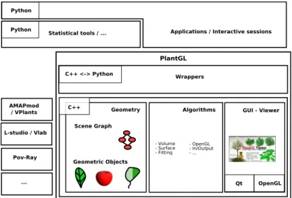
The overall architecture layout of PlantGL is shown in Figure 1, including sev-eral layers of encapsulation and abstraction. The geometric, algorithmic and GUI libraries lie in the core of PlantGL. The geometric library encapsulates a scene-graph data structure and a taxonomy of geometric objects. The algo-rithm library contains tools to manipulate and display geometric structures (for instance OpenGL rendering). The GUI is developed as a set of Qt widgets

and can be combined with the previous components to provide visualization facilities. On top of this first layer, a set of wrappers create interfaces of the C++ classes into the Python language using the Boost.Python library [38]. Because we design our C++ libraries in an oriented-object manner, the C++ class interfaces were totally compatible with the Python framework. All these interfaces are gathered into a Python module named PlantGL. Additionally, some automatic conversion tools with standard python structures were added into the wrappers in order to reinforce compatibility and integration. This module is thus integrated seamlessly with standard Python and enables fur-ther abstraction layers, written in Python. Extension of the library can be done using either C++ or Python.

Fig. 1. Layout of the PlantGL architecture. It contains three C++ components: a geometric, an algorithmic and a GUI library. On top of this, wrappers implement interfaces with the Python language. PlantGL primitives can be used by modellers to develop scripts, procedures and applications in the embedding language Python. Data structures can be imported from and exported to other plant modelling soft-ware systems mentioned on the bottom left.

2.3 Basic components

The basic components of PlantGL are scene-graphs that contain scene objects (geometry, appearance, transformation, etc.), actions that define algorithms that can be applied to scene-graphs, and the visualization tools.

2.3.1 Scene-graphs

Scene-graphs are a common data structure used in computer graphics to model scenes [39]. Basically, a scene-graph is a directed, acyclic graph (DAG), whose nodes hold the information about the elements that compose the scene. In a

DAG, nodes may have more than one parent, which enables parent nodes to share child nodes within the graph via the instantiation mechanism.

In PlantGL, an object-oriented version of scene-graphs was implemented to facilitate the customization of scene-graph node processing. Scene-graphs are made of nodes of different types. Types may be one of geometry, appear-ance, shape, transformation, and group. Scene-graph nodes are organized as a DAG hierarchy. Terminal nodes contain shapes pointing to both a geome-try node (which contains a geometric model) and an appearance node (e.g. which defines a color, a material or a texture). Non terminal nodes correspond to grouping or transformation nodes that allow the user to set the position, orientation and size of a geometric object. They are used to build complex objects from simple geometric models.

Two families of geometric models are available in the library: Explicit and Parametric models. Explicit models are defined as sets of discrete primitives like points, lines or polygons that can be directly drawn by graphics cards. Parametric models offer a higher level of abstraction and are thus simpler to manipulate. However, to be displayed, parametric models have to be trans-formed into an explicit representation. The discretization process is explicitly controlled by parameters of the models that indicate how many discrete prim-itives have to be created.

PlantGL contains a number of geometric models to represent points, curves, surfaces and volumes. They range from simple classical models such as Cylin-der, Sphere, and NURBS to more specific ones, e.g. Generalized CylinCylin-der, Hull, etc. Models dedicated to plant representation will be detailed in section 3.

2.3.2 Algorithms

In PlantGL, algorithms are separated from data structures for flexibility and reuse purposes. Given the heterogeneity of the nodes contained in the scene-graph, an algorithm applied to a scene needs to adapt its execution according to the type of node it is applied to. For this, we implemented the visitor design pattern [37] that makes it possible to keep algorithms outside node objects definition by delegating the mapping from node to algorithms to a separate visitor object called an action. It is thus possible to add new algorithms by implementing new actions without modifying the node classes or loosing per-formance (more details in appendix A).

In the actual implementation, PlantGL supports approximatively 40 actions that can be applied on a scene graph. The main ones can be classified into the following categories : converters, for instance from parametric to explicit representations; renderers; algorithms for the characterization of a scene using volume, surface or center of inertia; fitting algorithms to compute global

rep-resentations from a set of detailed shapes using for instance bounding volumes (sphere [40], box), convex hull [41]; ray casting using CPU or GPU; space parti-tioning e.g. in an Octree; etc. This last structure make it possible to determine quickly spatial neighbours to test for possible intersections between geome-tries, for instance during organ positionning in plant model generation [42]. A family of algorithms also makes it also possible to build and export a scene in different scene description formats: some classical ones, such as PovRay, Vrml, etc.or of some plant dedicated systems like AMAPmod/VPlants, LStudio/VLab, AMAPsimand VegeStar. This reinforces interoperability of PlantGL with other modeling tools.

The use of these algorithms is illustrated in section 4 in the context of different biological applications.

2.3.3 Visualization tools

The PlantGL Viewer (Figure 2) provides facilities to visualize scene-graphs interactively. Different types of rendering modes are available including volu-metric, wire, skeleton, and bounding box. Scene-graph organization and node properties can be explored with dedicated widgets allowing access to various pieces of information about the scene, like the number, volume, surface or bounding box of the scene elements. Simple editing features (such as a ma-terial editor) are available. Screen-shots can be easily made and exported to documents or assembled into movies. Most of the viewer features can be set using buttons or context menus and are also accessible procedurally.

Fig. 2. Visualization of the detailed representation of a 15 year old walnut tree [11] with the PlantGL viewer.

The viewer and scenes are multi-threaded so that a user can manipulate a scene from a Python shell during visualization. Several types of dialog boxes can also be interactively created in the Viewer from the Python shell. Results of the dialog are returned to the Python process using multi-threaded com-munications (see details in appendix A). This enables graphical control of a Python modelling process through the Viewer.

2.4 Creating scene-graphs

There are different ways for application developers to create and process a scene-graph depending both on performance constraints and their familiar-ity with computer graphics concepts. First, PlantGL provides a declarative language, GML [43], similar to VRML [44] with extensions for plant geometric objects. GML mainly adds persistence capabilities to PlantGL in both ascii and binary versions. For C++ applications, it is possible to link directly with the library. In this case, PlantGL features can also be extended by adding new objects and new actions. Additionally, the full PlantGL API is accessible from the Python language. Combination of high level tools and languages such as PlantGLand Python allows rapid prototyping of new models and applications, as illustrated in section 4.

3 Construction of Plant Models

The design of PlantGL is focused on modelling and rendering of vegetative scenes. In this section, we present the specific geometric models and modelling tools of PlantGL useful for the representation of plant components at different scales. In an increasing computational complexity, we examine sequentially the representation of simple plant organs, tree crown, branching systems and cellular representation of tissues.

3.1 Plant organs

To represent simple organs, PlantGL contains a set of classical geometric mod-els. For instance, some cylinders and frustums can be used to represent inter-nodes, NURBS patches to model complex organs such as leaves or flowers and generalized cylinders for branches and stems.

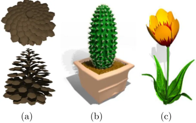
During the creation of a scene-graph, complex objects can be modeled using composition and instantiation. Simple procedures can be written in Python that position predefined symbols, for instance petals or leaves, using Trans-formation and Group objects, to create more complex objects by composition (Figure 3). Python, as a modelling language, allows the user to express a full range of modelling techniques. For instance, the pine cone (Figure 3.a) is built by placing each scale using the golden angle [45]. The following code2 _sketches the placement of each scale.

2 _{In all the code excerpts presented in this paper, standard python constructs are} formated in bold to emphasize the structure of the code and the names of the

(a) (b) (c)

Fig. 3. (a) a pine cone, (b) a cactus and (c) a tulip. Models were created with simple Pythonprocedures that create and position organs, like petals and leaves.

from p l a n t g l import ∗ p i n e = Scene ( )

s c a l e s m b = T r i a n g l e S e t ( . . . ) # Geometric symbol o f a p i n e s c a l e d e l t a a n g l e = p i /(1+ s q r t ( 5 ) ) # g o l d e n a n g l e b etw een each s c a l e n b s c a l e , m a x p i n e r a d i u s , m a x s c a l e s i z e = 1 6 0 , 5 0 , 1 . 5

b o t t o m h e i g h t , t o p h e i g h t = 1 0 , 90 # g l o b a l d i m e n s i o n s o f t h e p i n e def distToTrunk ( u ) : # w i t h u i n [ 0 , 2 ] , u < 1 f o r t h e bottom p a r t

i f u < 1 : return m a x p i n e r a d i u s ∗u e l s e: return m a x p i n e r a d i u s ∗((2 −u ) ∗ ∗ 2 ) def s c a l e S i z e ( u ) : i f u < 1 : return m a x s c a l e s i z e ∗ l o g (1+u , 2 ) e l s e: return m a x s c a l e s i z e ∗ l o g (3−u , 2 ) def s c a l e H e i g h t ( u ) : i f u < 1 : return u ∗ b o t t o m h e i g h t e l s e: return b o t t o m h e i g h t + ( u − 1 ) ∗ t o p h e i g h t f o r i in r a n g e ( n b s c a l e ) : u = 2∗ i / n b s c a l e p i n e += AxisRotated ( ( 0 , 0 , 1 ) , i ∗ d e l t a A n g l e , T r a n s l a t e d ( ( distToTrunk ( u ) , 0 , s c a l e H e i g h t ( u ) ) , S c a l e d ( s c a l e S i z e ( u ) , s c a l e s m b ) )

In this example, pine scales are identified by a normalized u position along the trunk with u ∈ [0, 1] for the bottom part and u ∈ [1, 2] for the top part. For a scale at position u, the functions distToTrunk, scaleSize and scaleHeight give the distance to the trunk, its size and its height respectively. Size of successive scales in the spiral follows a logarithmic law in this case. From this information and the golden angle, a geometric representation is built in the loop of the 5 last lines of code. Other algorithmic arrangements, such as the ones underlying Figure 3.b and c, can easily be made with python.

3.2 Crown models

3.2.1 Envelopes

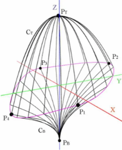
Tree crown envelopes are used in different contexts like studying plant inter-action with its environment (i.e. radiative transfers in canopies [10] or compe-tition for space [46]), 3D tree model reconstruction from photographs [7], and interactive rendering [47]. They are one original key application of PlantGL. In this section, we describe in detail three envelope models that were specifically designed to represent plant volumes: asymmetric, extruded and skinned hulls. Asymmetric Hull - This envelope model, originally proposed by Horn [48] and Koop [49], then extended by Cescatti [10], makes it possible to easily define asymmetric crown shapes. The envelope is defined using six control points in six directions and two shape factors CT and CB that control its convexity (see Figure 4). With a few easily controllable parameters, a large variety of realistic crown shapes can be achieved.

Fig. 4. Asymmetric hull parameters.

The first two control point, PT and PB, represent top and base points of the crown respectively. The four other points P1to P4represent the different radius of the crown in two orthogonal directions. P1 and P3 are constrained to lie in the xz plane and P2 and P4 in the yz plane. These points define a peripheral line L at the greatest width of the crown. For the x and y dimensions, L is composed of four elliptical quarters. The height of points of L is defined as an interpolation of the heights of the control points (see appendix B.1 for detailed equations).

The two shape factors CT and CB describe the curvature of the crown above and below the peripheral line. Points of L are connected to the top and base points with quarters of super-ellipse of degrees CT and CB respectively. Differ-ent shape factor values generate conical (Ci = 1), ellipsoidal (Ci = 2), concave

(Ci ∈]0, 1[), or convex (Ci ∈]1, ∞[) shapes. A great variety of shapes can be achieved by modifying shape factor values (see Figure 5).

Fig. 5. Examples of asymmetric hulls showing plasticity of this model to represent tree crowns (inspired by Cescatti [10]).

Cescatti proposed a simple methodology to measure the six control points and estimate the shape factors directly in the field. In PlantGL, a graphic editor has been implemented that makes it possible to build envelopes from photographs or drawings. For this, reference images can be displayed in the background of the different editor views. An illustration of this shape usage can be found for the interactive design of bonsai trees [30].

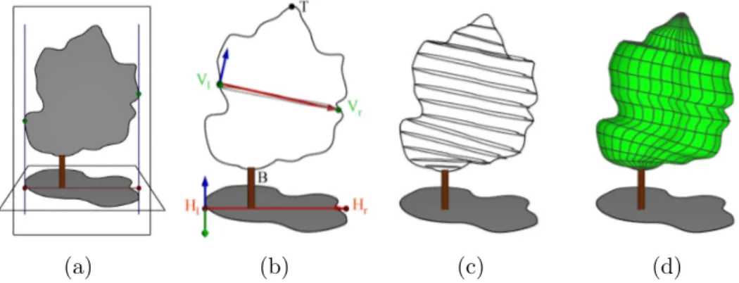
Extruded Hull - The use of extruded envelope for plant modelling was originally proposed by Birnbaum [50]. Such an envelope is defined with a horizontal and a vertical profile. This first profile can be acquired from the projection of a tree crown on the ground, given for instance by shadow on the field; and the second one from a lateral view of the tree.

(a) (b) (c) (d)

Fig. 6. Extruded Hull reconstruction. (a) Acquisition of a vertical and a horizontal profile. (b) Transformation of the horizontal profile into a section of the hull. (c) Computation of all sections (d) Mesh reconstruction.

The envelope is reconstructed by sweeping the horizontal profile inside the vertical profile (see Figure 6). For this, the vertical profile V is virtually split into slices by planes passing through equidistant points from the top (or by horizontal planes). These slices are used to map horizontal profiles inside V . Equations are given in appendix B.2.

An illustration of the reconstruction of such an envelope from photographs is given in section 4.1.

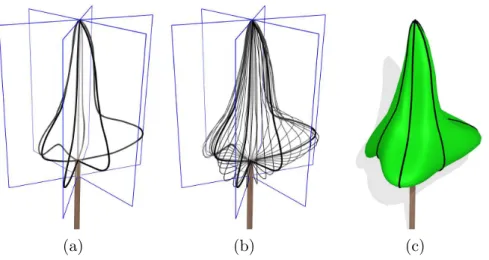
Skinned Hull -The previous envelope models account for variable radius of the crown in different directions but have limited input allowing variation of the profiles shapes to be captured. To alleviate this difficulty, we propose a new flexible profile based envelope model, namely skinned hull, which is defined as the interpolation of a set of vertical profiles given for any angle around the z-axis.

(a) (b) (c)

Fig. 7. Skinned Hull reconstruction. (a) The user defines a set of planar profiles in different planes around the z axis (in black). (b) Profiles are interpolated to compute different sections (in grey). (c) The surface is computed. Input profiles are iso-parametric curves of the resulting surface.

The skinned hull is inspired from skin surfaces [51–53]. It generalizes the notion of surface of revolution with a variational section being an interpolation of the various profiles (see Figure 7 and appendix B.3 for equations). For the particular case of a single profile, the surface is a surface of revolution.

3.2.2 Foliage distributions

In particular studies such as light interception in eco-physiology or pest prop-agation in epidemiology, only the arrangements of leaves in space is relevant. This lead us to define adequate means to specify leaf distributions indepen-dently of branching systems.

A first simple strategy consists of creating random foliage according to different statistical distributions. This can be easily expressed in PlantGL as illustrated by the following example. Let us consider a random canopy foliage whose leaf distribution varies according to the height in the canopy. The following code sketches the creation of three horizontal layers of vegetation with different statistical properties. In this example, leaves are generated above an hori-zontal rectangle delineated by (xmin,xmax) and (ymin,ymax). Layers Li are positioned between bottom and top heights (e.g. between heights[i − 1]and heights[i]). To simulate different leaf distributions in the foliage, we

asso-ciate an increasing probability to each height for a leaf to be above this height, bottom height of first layer having p0 = 0 and top height of last layer having p3 = 1. For the three layers, a leaf will thus have a probability p1 to be in the first layer, p2− p1 in the second layer, and 1 − p2 in the third one.

from random import uniform s c = Scene ( ) h e i g h t s = [ 1 , 2 , 3 , 4 ] # H e i g h t o f t h e l a y e r s l i m i t s l e a f s y m b o l = T r i a n g l e S e t ( . . . ) # Leaf geometry t o i n s t a n t i a t e f o r i in r a n g e ( n b l e a v e s ) : p = uniform ( 0 , 1 ) i f p <= p1 : h e i g h t = uniform ( h e i g h t s [ 0 ] , h e i g h t s [ 1 ] ) e l i f p1 < p <= p2 : h e i g h t = uniform ( h e i g h t s [ 1 ] , h e i g h t s [ 2 ] ) e l s e: h e i g h t = uniform ( h e i g h t s [ 2 ] , h e i g h t s [ 3 ] )

# random p o s i t i o n and o r i e n t a t i o n o f l e a v e s a t t h e chosen a l t i t u d e pos = ( uniform ( xmin , xmax ) , uniform ( ymin , ymax ) , h e i g h t )

az , e l , r o l l = uniform (−pi , p i ) , uniform ( 0 , p i ) , uniform (−pi , p i ) s c += T r a n s l a t e d ( pos , E u l e r R o t a t e d ( az , e l , r o l l , l e a f s y m b o l ) ) )

Figure 8 shows the resulting random foliage (trunk generation is not described in the code).

Fig. 8. A layered canopy foliage. The probabilities for a leaf to be in the first, second or third layer are respectively 0.1, 0.7 and 0.2 (giving p1= 0.1 and p2 = 0.8). Plant foliage may also exhibit specific leaf arrangement with regular and de-terministic properties. If the regularity corresponds to a form of spatial peri-odicity at a given scale, a procedural method similar to the previous one for random foliage can be easily used. However, some plants like ferns or pines show remarkable spatial organization of their foliage with several levels of aggregation and similar structures repeated at the different scales [15]. Such fractal spatial organizations can be captured by 3D Iterated Function Systems (IFS) [54].

An IFS is a set of contracting affine transformations {Ti}i∈[1,M ]. This family of contractions defines a contracting operator F for all bounded set of points

X in R3 _{such that:}

F (X) = T1(X) ∪ T2(X) ∪ . . . ∪ TM(X). (1) The F operator may be applied iteratively to an initial arbitrary 3D geomet-ric model, I, called the initiator . At the nth iteration the obtained object Ln has a pre-fractal structure composed of a number of elements increasing exponentially with n (while the size of each element decreases at an equivalent rate).

Ln = Fn(I) (2)

When n tends to infinity, the iteration process tends to a fractal object L∞, called the attractor. The attractor only depends on F (and not on the initiator) and has a known fractal dimension that depends on the contraction factors and number of F transformations, e.g. [55].

IFSs have been implemented in PlantGL as a transformation primitive. They may be used to construct reference virtual plant foliages with a priori deter-mined self-similar structures and dimensions, e.g. [15,34]. The following code shows the construction of the IFS of Figure 9. The affine transformations are defined as 4x4 matrices that are build here from a translation (t), a scaling factor (s) and a rotation defined from some euler angles (a). The initiator is a disk that represents a simple leaf shape.

t r a n s f o r m a t i o n s = [ Matrix4 . fromTransform ( t , s , a ) fo r t , s , a in [ ( ( 0 , 0 , 2 ) , 1 / 3 , ( 0 , 0 , 0 ) ) , ( ( 0 , 0 . 5 , 1 . 5 ) , 1 / 3 , ( 4 5 , 9 0 , 0 ) ) , ( ( 0 , − 0 . 5 , 1 . 5 ) , 1 / 3 , ( 4 5 , 2 7 0 , 0 ) ) , ( ( 0 . 5 , 0 , 1 ) , 1 / 3 , ( 4 5 , 0 , 0 ) ) , ( ( − 0 . 5 , 0 , 1 ) , 1 / 3 , ( 4 5 , 1 8 0 , 0 ) ) , ( ( 0 , 1 , . 5 ) , 1 / 3 , ( 4 5 , 9 0 , 0 ) ) , ( ( 0 , − 1 , . 5 ) , 1 / 3 , ( 4 5 , 2 7 0 , 0 ) ) , ( ( 1 , 0 , 0 ) , 1 / 3 , ( 4 5 , 0 , 0 ) ) , ( ( − 1 , 0 , 0 ) , 1 / 3 , ( 4 5 , 1 8 0 , 0 ) ) ] ] i = IFS ( 4 , t r a n s f o r m a t i o n s , Disk ( 1 ) )

3.3 Branching system modelling

3.3.1 Scene-graphs for plants

In PlantGL, the construction of a branching system comes down to instanti-ating a p-scene-graph. A p-scene-graph corresponds to an adaptation of the PlantGL scene-graph to the representation of plant branching structures. For this, a particular set of nodes in the p-scene-graph, named structural nodes, are introduced and represent the different components of the plant. These

(a) (b) (c)

Fig. 9. Construction of a fractal foliage using an IFS. (a) The initiator is a disc (rep-resenting a leaf shape). In the first iteration, the initiator is duplicated, translated, rotated and resized according to the affine transformations that compose F , leading to L1. (b-c) IFS foliages L3 and L5 at iteration depths 3 and 5. The theoretical dimension of this foliage is 2.0

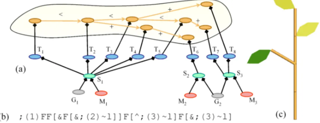
nodes are organized as a tree graph (as described in [56]) in which two types of edges can be specified to distinguish branching (+) and succession (<) rela-tionships between parent and child nodes (see Figure 10.a). In addition, each structural node is connected with transformation, geometry and appearance nodes that define the representation of each component. In p-scene-graphs, transformations can either be specified in an absolute or relative mode. In the absolute mode, transformations are expressed with respect to a common global reference frame whereas, in the relative mode, transformations are expressed in the reference frame of the parent component in the tree graph.

Fig. 10. A p-scene-graph. (a) The scene-graph with structural nodes in orange, transformation in blue, shape in green, appearance in red and geometry in grey. (b) The corresponding L-systems bracketed string from which it has been constructed. The ’F’ symbols are geometrically interpreted as cylinders, ’∼l’ as leaf symbols, ’&’ and ’^’ as orientation operations and ’;’ as color specifications, [57]. (c) The corresponding geometric model.

The topological relationships specified in the p-scene-graph express physical connections between plant components. For this, a set of constraints, namely

within-scale constraints, can formalize these connections in term of geome-try [26]. These constraints may specify for instance continuity relationship between the geometric parameters of connected components (end points, di-ameters, etc.). These constraints are used to ensure the consistency of the overall representation.

P-scene-graphs are further extended by introducing a multiscale organization in the structural nodes, which makes it possible to augment the multiscale tree graphs (MTG) used in plant modelling [56] with graphical informations [58]. Such multiscale graphs correspond to recursively quotiented tree graphs [56]. It is possible to define multiscale organization from a simple detailed tree graph (namely the support graph) by specifying quotient functions that will partition the nodes into groups corresponding to macroscopic components in the MTG.

The different scales included in the multiscale p-scene-graph give different views with different resolutions of the same plant object. Since they corre-spond to different views of the same reality, the associated geometric models must respect particular coherence constraints. For this, a set of between-scale constraints is defined that relate the model parameters at one scale with the model parameters at other scales. Between-scale constraints may specify for instance that all the components of a branching system must be included in some macroscopic envelope. These constraints may be either used in a bottom-up or top-down fashion. In top-down approaches, macroscopic representation may be used to bound the development of a plant at a more microscopic level. Such a strategy was used for instance in [30] for the design of bonsai tree using L-systems. In bottom-up approaches, a detailed representations of a plant is used to compute a more macroscopic representation. For this, a set of fitting algorithms has been implemented in PlantGL that makes it possible to compute the bounding envelope of a set of geometric primitives using for instance convex hulls [41] or minimal bounding sphere [40], etc. These enve-lope representations can thus be used to characterize globally the geometry of a branching system at different scales, for instance for computing the fractal dimension of a plant [15].

3.3.2 Construction of branching structure models

P-scene-graphs can be created either by generative procedures written in Python or by importing plant structures from other plant modeling software. From a generative perspective, we particularly emphasized in the current ver-sion of PlantGL the connection with studio/VLab [6], a widely used L-system based modelling framework for plant growth modelling. An L-L-system [3] is a particular type of rewriting system that may be used to simulate the

development of a tree like structure. In this framework, the tree structure is encoded as a bracketed string of symbols called modules that represent com-ponents of the structure. To represent attributes, these modules may bear parameters. Particular bracket symbols mark the beginning and the end of branches. The plant growth is formalized by a set of production rules that describes the change over time of the string modules. Starting from an ini-tial string, namely the axiom, modules of the string are replaced according to appropriate rules. A derivation step corresponds to the rewriting in parallel of every module of the string. Therefore, the development of a tree structure through time is modelled by a series of derivation steps. To associate a geomet-ric interpretation with the L-system’s output string, some modules are given a graphical meaning and a LOGO-style turtle is used to interpret them, [59]. For this, the string is scanned sequentially from left to right and particular modules are interpreted as actions for the turtle. The turtle state is charac-terized by a position, a reference frame and additional graphical attributes. Some modules make the turtle move forward and draw graphical elements (cylinders, etc.) or change its orientation in space. A stack mechanism makes it possible to store the turtle state at the beginning of a branch and to restore it at the end.

In order to interface L-studio/VLab with PlantGL, import procedures have been implemented in PlantGL. The strings representing the branching systems generated with cpfg are stored in text files. These strings are then imported into PlantGL with the dedicated primitive Lstring. To interpret the L-system modules as commands for the creation of a p-scene-graph, a particular turtle has been implemented in PlantGL that follows the Lstudio/VLab specification [3] (see Figure 10). Since the p-scene-graph is accessible in Python, it is then possible to interactively explore and analyse the resulting geometric structure with the set of algorithms available in PlantGL for the manipulation of a scene-graph or for the analysis of a plant topological structure using other toolkits such as AMAPmod/VPlants [60]. The following code sketches the import of a L-system string in PlantGL, its conversion into a scene-graph and some basic manipulation of the result such as display and wood volume computation.

l s t r i n g = L s t r i n g ( ’ p l a n t . s t r ’ ) t u r t l e = P g l T u r t l e ( ) l s t r i n g . apply ( t u r t l e ) s g = t u r t l e . getSceneGraph ( ) Viewer . d i s p l a y ( s g ) v o l = volume ( s g )

A more complex example of such a coupling between Lstudio/cpfg and PlantGLis illustrated in section 4.3.3. It uses PlantGL’s hulls defined in section 3.2.1 to constrain L-systems generation of branching structure. Other connec-tions with modelling platforms such as AMAPmod/VPlants [26], and VegeSTAR

(a) (b) (c)

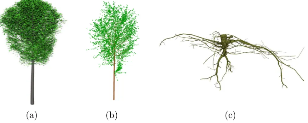
Fig. 11. Example of branching systems in PlantGL. (a) A beech tree simulated with an L-system using Lstudio/VLab and imported in PlantGL. This model is used in the application presented in section 4.3.3. (b) Black tupelo tree generated procedu-rally in Python using PlantGL according to the generative procedure proposed by Weber and Penn in [4] and (c) the root system of an oak tree [13].

[61] are also available and make it possible to create 3D plant models from measured data (see Figure 11).

3.4 Tissue models

In PlantGL, a plant tissue is considered as a collection of connected regions. A region may represent either a single cell or a set of cells. Unlike branch-ing systems, the neighborhood relationship between regions cannot be simply represented by tree graphs since the connection networks between regions usu-ally contain cycles. To model the neighborhood relationship between regions correctly, we need to take into account the hierarchical organization of region connections: for example, in 3 dimensions, two 3-D cells are connected through a 2-D wall, two walls are connected through a 1-D edge and two edges are con-nected through a 0-D vertex. More generally, the connection between two or more elements of dimension n + 1 is an element of dimension n. Such a hier-archical organization defines an abstract simplicial complex [62]. Similarly to p-scene-graphsfor branching systems, scene-graphs representing tissues, called t-scene-graphs, are defined by augmenting simplicial complexes representing cell networks with geometrical properties. Each structural node of the sim-plicial complex is associated with transformation, geometry and appearance nodes.

A set of geometric algorithms has been designed to simplify the manipulation of the t-scene-graphs during simulations.

• The first algorithm makes it possible to define the geometry of an element of dimension n + 1 from the geometric information of its components of

a b c d

Fig. 12. Tissue models. (a) 2D tissue, (b) 2D transversal cut, (c) 3D surface tissue from [33], (d) 3D tissue.

dimension n. For example, the polyhedral geometry of a cell is derived from the polygonal geometry of its walls. The overall consistency of the geometry of all elements in the tissue is thus ensured by specifying only the geometry of its smallest elements.

• The second algorithm implements cell division. A cell (or more generally a region) is divided in two daughter cells. The geometry of these daughter cells may be specified by the user using standard PlantGL algorithms (that compute main axis, shape volume or surface, shape orientation, ...) to reflect the biological characteristics of cell division geometry (main orientation of the cell, smallest separation wall, orthogonality between walls, ...).

• The third algorithm has been designed to refine t-scene-graphs into small triangular elements. Resulting meshes can be used either to visually dis-play the tissue or in conjunction with finite element methods to solve dif-ferential equations representing physiological processes (diffusion, reaction, transport,...) or mechanical stresses for example.

T-scene-graphs can be obtained either from a file, from images of biological tis-sues [33], or using procedural algorithms. PlantGL provides a set of procedural algorithms that generate regular, grid-based tissues (based on rectangular or hexagonal grids) and non-regular tissues containing cells with random sizes. Random tissues are generated using a randomly placed set of points represent-ing cell centers. The Delaunay triangulation (2D or 3D) of this set of points is then computed. This is done by using an external computational geometry library, CGAL [63], available in Python. Cell neighborhood is defined by this tri-angulation and walls correspond to its dual representation (Vorono¨ı diagram). These procedural algorithms result in relatively simple tissue structures. More complex t-scene-graphs can be obtained by simulation of tissue development. Starting from an initial simple tissue, a growth algorithm modifies the shape of the tissue. A cell is divided each time its volume reaches a given threshold. This combination of growth and division is maintained up to the desired final shape (see 4.3.1 for example).

4 Applications and Illustrations

The PlantGL library has already been used in a number of modeling appli-cations by our group (e.g. [33,34,15,31,36]) and other plant research groups (e.g. [32,35]). The library allows modellers to address graphic and geometric issues in the different phases of a modeling process, i.e. observation, anal-ysis, simulation and model evaluation. In this section, we aim to illustrate how PlantGL provides a set of useful efficient tools to address various ques-tions in these different phases. In particular, we stress the use of envelope- or grid-based approaches which is original in PlantGL and opens new application areas. In these applications, we illustrate how PlantGL can be assembled with other Python libraries to achieve high-level operations on plant structures, thus opening the way to the definition of a powerful plant modeling platform.

4.1 Plant Canopy Reconstruction

In plant modeling, 3D digitizing of plant structure has become a topic of increasing importance in the last decade. Various methodologies have been used to digitize plants at different levels of detail for leaves, for branching systems, and also for tree crowns [64,65,26,50,7,46]. Among these approaches, the reconstruction of 3D models of large/tall trees (like trees of a tropical forest for example) remains a challenging problem. This is mainly due to the difficulty of acquiring information in the field, and in capturing the intricate structure of such plants. In this section, we show how the new envelope-based tools provided in PlantGL can be used for this aim.

4.1.1 Using PlantGL to build-up large crowns

First approaches attempted to use parametric models to estimate the geometry of tree crowns in the context of light modeling in plant stands [10]. More recently, non-parametric visual hulls have been used in different application contexts to characterize the plant volume based on photographs [7,47,46]. PlantGLmakes it possible to easily combine these approaches by using for ex-ample photographs and parametric envelope models to estimate plant canopy volumes.

Using a set of images of a tree (being either photographs or botanical drawings) with known camera positions and orientations, the modeler has to define a number of crown profiles according to the selected envelope model. For the extruded hull for instance, two closed curves that encompass the entire crown in vertical and horizontal planes are required. This step is usually made by

(a) (b) (c)

Fig. 13. Reconstruction of the crown envelope of a Schefflera Decandra tree with an extruded hull built from two photographs. Sketches are done with an internal curve editor. Photo courtesy of Y. Caraglio.

manually outlining the foliaged tree region using an internal curve editor. Profiles are then used to build the tree silhouette hull.

From this estimated crown envelope, the modeler can then infer a detailed crown model by making assumptions about the leaf distribution inside the crown. Figure 13 illustrates the use of a simple uniform random distribution of leaf positions and orientations. The following code shows how the example for random foliage generation of section 3.2.2 can be adapted to take into account complex crown shapes.

h u l l # r e c o n s t r u c t e d h u l l bbx = BoundingBox ( h u l l )

f o l i a g e = Scene ( ) def r a n d o m p o s i t i o n ( ) :

return ( uniform ( bbx . xrange ( ) ) , uniform ( bbx . yrange ( ) ) , uniform ( bbx . z r a n g e ( ) ) )

f o r i in r a n g e ( n b l e a v e s ) : pos = r a n d o m p o s i t i o n ( ) while not i n s i d e ( h u l l , pos ) :

pos = r a n d o m p o s i t i o n ( )

f o l i a g e += T r a n s l a t e d ( pos , l e a f s y m b o l ) )

leaves is made in 1 sec. on a Pentium IV 2.0 GHz3_{. Using Python, it is} possible to define foliage distribution using more complex algorithms, such as those described in [6,7,30].

4.1.2 Using PlantGL to assess plant mock-up accuracy

Another important problem in canopy reconstruction is to assess the accuracy of 3D plant mockups obtained from measurements. A family of solutions con-sists of comparing equivalent synthesized descriptions of both the real and the virtual plants. In this family, hemispherical views are particularly interesting since they directly measure a physical characteristic of the plant, namely the amount of intercepted light.

Figure 14 illustrates this approach [66]. A hemispheric picture is taken from the real plant, while an equivalent virtual picture is computed with the same camera position on the reconstructed plant. White areas in both pictures di-rectly reflect the amount of light that reach different positions under or inside the crown [67]. The amount of intercepted light is summarized with the canopy openness index defined as the ratio between white pixels and total number of pixels on the picture.

Fig. 14. Assessment of plant model reconstruction using hemispheric view [66]. The Juglans nigra x Juglans regia hybrid walnut plant model is reconstructed from par-tial measurements: wood structure is manually digitized while leaves are generated from distribution functions. On the left, an hemispheric photograph of a real wal-nut from the ground. On the right, reconstructed mockup using AMAPmod/VPlants exported to Pov-Ray [68] to compute a hemispheric picture at the same position. Here, the evaluated canopy openness is 40% for the real photograph and 49 % for the virtual tree.

3 _{The computation times indicated in the remainder of this paper are for the same} hardware configuration.

4.2 Analysis of Plant Geometry

Plant geometry is a parameter of paramount importance in the modeling of plant-environment interactions. However, plants usually show complex geo-metric shapes with numerous components, highly organized but with non-deterministic structure. Characterizing this “irregularity” of plant shapes with few high level parameters is thus a determinant issue of modeling approaches. In many applications in forestry, horticulture, botany or eco-physiology, anal-ysis of plant structures are carried out to find out adequate ways of capturing their intricate geometry in simple models. In this section, we illustrate the use of grids and envelopes defined in PlantGL in order to achieve such analysis.

4.2.1 Grid-Based Analysis

Fractal geometry was introduced to analyse the geometry of markedly irreg-ular structures that can be either mathematically constructed or found in nature [69]. Several parameters have been introduced for this purpose, such as fractal dimension and lacunarity. These parameters are intended to cap-ture the essence of irregularity, i.e. the way these struccap-tures physically occupy space as resolution decreases. Several estimators of these parameters exist. They consist of paving the original object in different manners with tiles of different sizes and studying the variation of the number of tiles with tile size.

Fig. 15. The box counting method applied to the foliage of a digitized apple tree [70]. The tree is 2m height with around 2500 leaves. Global bounding box has a volume of 10 m3 and serves as the initial voxel. A grid sequence is then created by subdividing uniformly this bounding box into sub-voxels. At each scale, intercepted voxels are counted to determine fractal dimension (here of the order of 2.1). For plant structures, fractal properties, such as fractal dimension, have been computed in different contexts, e.g. [71]. They frequently rely on the fractal analysis of 2D photographs. However, more recently, several works showed the possibility to compute more accurate estimators using detailed 3D-digitized plant mock-ups of real plants [72,15,34].

PlantGL makes it possible to carry out such computation in a flexible way. For example, to implement the box-counting estimator of the fractal dimension [69], the PlantGL “grid” object can be used to count the number of 3D cells of a given size containing vegetation. If N (δ) denotes the number of occupied 3D cells of size δ, the box-counting estimator of the fractal dimension Dδ of the object is defined as:

Dδ = lim δ→0 ln N (δ) ln1 δ . (3)

Dδ is estimated from the slope of the regression between ln N (δ) and ln 1_δ values. The following code sketches the implementation of such an estimator using Python and PlantGL.

from s c i p y import s t a t s def b o x c o u n t i n g ( s c e n e , m a x d i v i s i o n ) : n b v o x e l s = [ l o g ( Grid ( s c e n e , d i v ) . n b i n t e r c e p t e d v o x e l s ( ) ) f o r d i v in r a n g e ( m a x d i v i s i o n ) ] d e l t a =[ l o g ( 1 . / i ) fo r i in r a n g e ( m a x d i v i s i o n ) ] s l o p e , i t c e p t , r , ttp , s t d e r r=s t a t s . l i n r e g r e s s ( n b v o x e l s , d e l t a ) return s l o p e # s l o p e o f t h e r e g r e s s i o n

Figure 15 illustrates the application of the box counting method on the foliage of a 3D-digitized apple tree [70]. For this example, computation of the 30 grids of decreasing sizes took 0.7 sec. PlantGL can be used in a similar way to compute various fractal properties of plants [15,34]

4.2.2 Envelope-Based Analysis

Parametric envelopes provided in PlantGL can also be used to analyse vol-umetric properties of plant crowns. For example, in order to quantify the development of a plant crown over time, envelopes can be adjusted to the crown of the developing tree at different ages and their surface or volume can then be estimated.

Figure 16 illustrates this approach together with the possibility to import plant data from other software. The growth of a eucalyptus was simulated at various ages using the AMAPsim software [23], Figure 16.a. Results were imported in PlantGL as MTGs. The convex hull of the plant crown was then computed at each age using the fitting algorithms provided by PlantGL for envelopes. Here is how this series of steps can be carried out in PlantGL: import pylab

def h u l l a n a l y s i s ( ages , t r e e s ) :

(a) (b)

(c)

Fig. 16. (a) A eucalyptus tree simulated at various age (from 1 to 8 months on a scale from 10 to 250) with the AMAPsim software, exported to PlantGL and rendered with Pov-Raysoftware [68] (b) Global representations of eucalyptus crown at the various ages (c) Increments of wood and hull surfaces over time. The different degrees of correlation and their associated time period enable us to identify the various phases of the crown development.

w o o d s f =[ s u r f a c e ( i ) for i in t r e e s ] h u l l s f =[ s u r f a c e ( i ) fo r i in h u l l s ] d e l t a w o o d s f =[ w o o d s f [ i +1]− w o o d s f [ i ] fo r i in r a n g e ( l e n ( w o o d s f ) −1)] d e l t a h u l l s f =[ h u l l s f [ i +1]− h u l l s f [ i ] fo r i in r a n g e ( l e n ( h u l l s f ) −1)] pylab . p l o t ( a g e s [ 1 : ] , d e l t a w o o d s f ) pylab . p l o t ( a g e s [ 1 : ] , d e l t a h u l l s f )

Based on such data, various investigations about the crown development can be made. Curves showing the variation of crown surface/volume through time can be analysed as shown in Figure 16.c. Comparison at a more microscopic scale with the leaf area variation can thus be made.

4.3 Simulations based on plant geometric models

The use of flexible geometric models of plants is not restricted to the analysis of plant structure. They can be used as well for the simulation of various physical or physiological processes that take place within or in interaction with the plant structure. Here, we present three applications that demonstrate the use of PlantGL at different scales, ranging from organ to communities.

4.3.1 Simulation at organ scale

Due to the recent advances in plant cellular and developmental biology, the modeling of plant organ development is considered with a growing interest by the plant research community: leaf [73–75], shoot apical meristem [76–80], and flower [81]. PlantGL provides flexible data structures and algorithms that make it possible to develop 2D or 3D simulations of tissue development. As a matter of illustration, let us model the development of a bump forma-tion in a tissue for instance to simulate development of a primordium at a shoot apex. We assume that the tissue is composed of polygonal cells in 2D (respectively polyhedral cell in 3D) delimited by 1D walls in 2D (respectively by polygonal walls in 3D).

The bump formation of a primordium at the surface of a meristem can be approximated (in cylindrical coordinates) by :

z(r, t) = h(t)

1 + ek(r−rm(t)) (4)

where h is the height of the bump, rm is the radius of the bump at half its height and k is a shape factor that defines the slope of the bump. h and rm vary throughout time at a rate ρh and ρr respectively. From this equation we can derive a time dependent velocity field for surface vertices. The velocity of the internal vertices is an interpolation between the surface velocity and the velocity of the most inner vertices. To simplify, we assume that the most inner vertices (at altitude zmin) are fixed and their speed is then equal to zero. At each time t of the simulation, each vertex is moved according to its velocity. This process progressively modifies the cell size, and consequently the overall tissue shape. During the growth, if a cell has a volume (or surface in 2D) that reaches a predefined threshold, it divides into two children cells. Different algorithms implementing cell division are available on a tissue object, e.g. [82]. Here follows the code of such a tissue growth in PlantGL for a particular choice of the cell division algorithm :

t i s s u e = c r e a t e G r i d T i s s u e ( ( 2 0 , 5 ) ) def s u r f a c e a l t i t u d e ( r , t ) :

return h ( t )/(1+ exp ( k ∗ ( r−rm( t ) ) ) ) def v e l o c i t y f i e l d ( pos , t ) :

r=norm ( pos . x , pos . y ) tmp=exp ( k ∗ ( r−rm( t ) )

s u r f a c e s p e e d =( r h o h ( t )+k∗h ( t ) ∗ r h o r ( t ) ∗ tmp/(1+tmp))/(1+tmp ) z s p e e d=s u r f a c e s p e e d ∗ ( pos . z−zmin ) / ( s u r f a c e a l t i t u d e ( r , t )−zmin ) return Vector3 ( 0 , 0 , z s p e e d )

f o r pos in t i s s u e . p o s i t i o n s ( ) :

pos+=v e l o c i t y f i e l d ( pos , t ) ∗ d e l t a t i m e f o r c e l l in t i s s u e :

i f c e l l . s i z e ( ) > m a x c e l l s i z e : c e l l D i v i d e ( c e l l , a l g o=MAIN AXIS)

Results of the simulation are presented on figure 17. This growth simulation of the tissue, composed of 100 cells, using 100 time iterations took 4.5 sec. Note that interpolation has been slightly modified to account for a constant size of the two external layers of cells.

(a) (b) (c)

(d)

Fig. 17. (a,b,c) 2D geometrical representation of a growing tissue at three different times. (d) 3D simulation of bump formation on a tissue

4.3.2 Simulation at plant scale

In biological applications, virtual plants are frequently used to carry out vir-tual experiments where data is difficult to measure or when the interaction between the studied processes is too complex. This is particularly true for the study of light interception by plants: light cannot be measured in a real canopy with high accuracy and the amount of light rays that can go through a canopy is a complex function of the tree architecture. While the canopy openness index presented in section 4.1.2 gives an estimation of the ratio of light intercepted by the plant from one view point, this example addresses the problem of integrating such a measure on the whole plant structure. Addition-ally, it illustrates the use of PlantGL in the context of model assessment and shows how high-level geometric operations used in light interception models can be simply performed with PlantGL.

Surface to Total Area Ratio [83]. This eco-physiological parameter is a direc-tional quantity defined by taking the ratio of the area of the projection of a tree foliage SΩ in a particular direction Ω to its total leaf area S. The STAR is thus the mean irradiance of a leaf area unit.

ST ARΩ = SΩ

S (5)

The directional STAR index can be integrated over all the sky vault to char-acterize the overall light interception of a tree. For this, a set of directions given by the turtle sky discretization [84] can be used and associated STAR values are averaged after weighting by the standard overcast sky radiance distribution [85].

Since the total leaf area of a real plant is often expensive to measure, approxi-mate values of the STAR are often used in eco-physiological applications. For this, the directional STAR is estimated from simple measures of the plant volume and leaf density and by making simplifying assumptions on the actual spatial distribution of leaves in the canopy [86]. In this case, the plant is sup-posed to be a homogeneous volume with small leaves uniformly distributed within the crown looking like a “turbid medium”. In this context, a light beam b of direction Ωb has a probability p0(b) to be intercepted :

p0(b) = exp (−GΩb.LAD.lb) (6)

where GΩb is a coefficient characterizing the spatial distribution of leaf

orienta-tions in the crown volume, LAD is the Leaf Area Density in the volume and lb the length of the beam path in the crown volume. Assuming the B beams con-stitute a regular and dense sampling of the whole volume, the approximated directional STAR of the turbid volume, \ST ARΩ, can then be computed as [87]: \ ST ARΩ = B X b=1 Sb(1 − p0(b))/S (7) where Sb is the cross section area of a beam. This model-based definition of the STAR can be compared to STAR from Equation 5 to evaluate the quality of light model assumptions. The resulting difference characterizes the error due to the model’s underlying hypotheses (homogeneity/randomness of the foliage distribution, negligibility of leaf size, ...) with respect to the actual canopies [86].

turbid-medium-based STARs, can be computed from a plant mockup using the high-level library functions. The projection based STAR of a given virtual canopy can be computed by counting the number of vegetation pixels in a virtual picture obtained by projecting virtual plant canopies using an orthographic camera [86] and multiplying by the size of a pixel. This would be expressed as follows in PlantGL: def s t a r ( l e a v e s , d i r ) : Viewer . d i s p l a y ( l e a v e s ) Viewer . camera . s e t O r t h o g r a p h i c ( ) Viewer . camera . s e t D i r e c t i o n ( d i r ) p r o j , n b p i x e l , p i x e l s i z e = Viewer . frameGL . g e t P r o j e c t i o n S i z e ( ) return p r o j / s u r f a c e ( l e a v e s )

For the turbid medium based STAR, the envelope of the tree crown must first be computed. Then, a set of beams of direction Ω are cast and their interceptions and resulting length in the crown volume are computed. A sketch of such a code would be as follows:

def s t a r ( l e a v e s , g , d i r , up , r i g h t , b e a m r a d i u s ) : h u l l= f i t ( ’ c o n v e x h u l l ’ , l e a v e s ) l a d = s u r f a c e ( l e a v e s ) / volume ( h u l l ) bbx = BoundingBox ( h u l l , d i r , up , r i g h t ) Viewer . d i s p l a y ( h u l l ) pos = bbx . upperRightCorner ( ) i n t e r c e p t i o n = 0 f o r r s h i f t in r a n g e ( bbx . s i z e ( ) . y/ b e a m r a d i u s ) : f o r u p s h i f t in r a n g e ( bbx . s i z e ( ) . z / b e a m r a d i u s ) :

i n t e r s e c t i o n s = Viewer . castRay ( pos−r s h i f t ∗ r i g h t −u p s h i f t ∗up , d i r ) p0 = 1 f o r i n t e r s e c t i o n in i n t e r s e c t i o n s : l e n g t h = norm ( i n t e r s e c t i o n . out−i n t e r s e c t i o n . in ) p0 ∗= exp(−g∗ l a d ∗ l e n g t h ) i n t e r c e p t i o n += (1−p0 ) ∗ ( b e a m r a d i u s ∗ ∗ 2 ) return i n t e r c e p t i o n / s u r f a c e ( l e a v e s )

with intersection containing the in and out intersection points of the ray and a hull and intersections being a list of such structure. The STAR with ray casting took 0.3 sec for each direction to be computed with PlantGL and the approximated one took 10 sec using 50000 rays.

4.3.3 Simulation at community scale

Detailed plant models, at the level of branches and leaves, do not always cor-respond to the most adequate level for expressing knowledge in plant models. PlantGL provides a number of ways to deal with abstract representation of

(a) (b) (c)

Fig. 18. Light intercepted by an apple tree represented as shadow on the ground. Intensity of the colors represent intensity of interception. STAR can be computed as a ratio between the area of the shadow and the plant leaf area. (a) Light intercepted from top direction using ray casting. STAR in this direction is equal to 0.23 (b) Light intercepted from same direction using Beer-Lambert hypothesis. STAR in this case is equal to 0.34. (c) Light interception sampled from different directions. The different colors are used to mark the difference between various elevations of ray direction. Sky integrated STAR is equal in the case of ray casting to 0.44 and in the case of Beer-Lambert to 0.58. This confirms that the turbid medium hypothesis over-estimates the STAR measure [86].

plants at different scales. In particular, the various envelope models defined in section 3.2.1 can be used as abstract means to model plant crown bulk. Such models are useful for instance in the modeling of plant communities, where competition for space has been shown to be a key structuring factor [88]. In the following example, we illustrate how natural scenes containing thou-sands of plants distributed in a realistic manner can be built with PlantGL, taking into account competition for space. It is inspired by [31] which is an extension of [89,90] to the use of more complex crown shapes.

The ecosystem synthesis starts with the generation of a set of coarse individu-als with height, crown radius and crown base height determined from density and allometric functions.

Individuals are fagus beech trees with different classes of ages. Allometric functions of the Fagac´ees model [91] are used to determine the heights and radius values as a function of tree age. The spatial distribution of these plants is generated using a stochastic point process. For this, we use a Gibbs process [92,93] defined as a pairwise interaction function f (pi, pj), that represents the cost associated with the presence of two given plants at positions pi and pj respectively. Positive cost values will lead to repulsion between trees while negative ones lead to attraction. A realization of this process is intended to minimize the global cost F = P

associated with each pair of points. The Gibbs process is simulated with a classical depletion-replacement iterative algorithm [94].

Classically, the cost function is used to model neighbor competition and is defined as a function of the crown radii and positions of the trees. The cost function of two trees i and j, characterized by shapes with constant radius, may be chosen for instance proportional to the difference between the sum of the crown radii and the distance between pi and pj. For asymmetric shapes, the same function can be used where radii of trees now correspond to the radius of each envelope in the direction defined by the tree positions pi and pj. In addition, both the position and the different parameters of the crown envelope can now be changed in the depletion-replacement algorithm. Figure 19 illustrates the 3D output of such a process.

Fig. 19. A front and top view of a generated stand at the crown scale. Different colors are used to differentiate various layers of vegetation.

From this set of coarse individuals, detailed plant representations can be in-ferred and assembled into a complete scene. For this, different generation meth-ods either available in PlantGL or outside of the software can be used. In our example, we generated the beech trees with the L-systems models using the generative procedure described in [30]. Bushes and flowers were generated us-ing PlantGL and Python as presented in section 3.3 and added to the scene. Finally, a digitized walnut tree [65] was also added to illustrate how scenes may be created in PlantGL using a range of classical date sources.

The final rendering was made with Povray [68]. Each plant geometric model was converted and assembled in this format. Figure 20 illustrates the resulting scene. The computation of the distribution of the 56 trees on the terrain using the depletion-replacement algorithm with 4000 iterations is made using pure Python and took 5 min. Generation of individual tree structure using L-systems took 20 sec per tree. The final Povray rendering took 5 min.

Fig. 20. A community of plants generated from a Gibbs process [31]. The scene is made of plants from different sources: beech trees of different sizes and ages where generated using the ecosystem model presented in section 4.3.3. A walnut tree corresponding to a 3D digitizing of a real plant built using AMAPmod/VPlants, virtual bushes flowers and grass created procedurally in Python with PlantGL 5 Conclusion

In this paper, we presented a new open-software library for the geometric modeling of plants built on the top of the Python programming language. The library provides a set of geometric models that are useful to represent various types of plant structures at different scales, ranging from tissues to plant communities. In particular, it contains original geometric components such as dedicated parametric envelopes for crown shape representation and tissues for representing plants at cell scale in 2D or 3D. Branching systems can be created either procedurally or by importing them from plant growth simulation platforms, such as LStudio/VLab. The resulting plant geometric models can be easily analysed using Python and PlantGL high level algorithms. The different features of the PlantGL library have been illustrated on applications involving plants at different scales and showing its use at various stages of a modeling process.

Acknowledgments.

The authors thank P. Prusinkiewicz for kindly making the LStudio/VLab software available to them, D. Da Silva for STAR computation on the apple tree and the shadow images, P. Barbier de Reuille and Y. Caraglio for their contribution to some images, and H. Sinoquet, E. Costes, F. Danjon, C.-E.