HAL Id: cirad-00189405
http://hal.cirad.fr/cirad-00189405
Submitted on 20 Nov 2007HAL is a multi-disciplinary open access
archive for the deposit and dissemination of sci-entific research documents, whether they are pub-lished or not. The documents may come from teaching and research institutions in France or abroad, or from public or private research centers.
L’archive ouverte pluridisciplinaire HAL, est destinée au dépôt et à la diffusion de documents scientifiques de niveau recherche, publiés ou non, émanant des établissements d’enseignement et de recherche français ou étrangers, des laboratoires publics ou privés.
Simulation Model
Pedro S. Fortes, Luís S. Pereira, António A. Campos
To cite this version:
Pedro S. Fortes, Luís S. Pereira, António A. Campos. GISAREG - A GIS Based Irrigation Scheduling Simulation Model. Séminaire sur la modernisation de l’agriculture irriguée, 2004, Rabat, Maroc. 13 p. �cirad-00189405�
Modernisation de l’Agriculture Irrigu´ee Rabat, du 19 au 23 avril 2004
GISAREG - A GIS Based Irrigation Scheduling
Simulation Model
Pedro S. Fortes1, Lu´ıs S. Pereira1, Ant´onio A. Campos1
1 Center for Agricultural Engineering Research, Institute of Agronomy, Technical University of Lisbon,
Portugal
E-mail :[email protected]
Abstract - ISAREG is a conceptual non-distributed water balance model for simulating crop ir-rigation schedules at field level and to compute irir-rigation requirements under optimal and/or water stressed conditions. To support the users of ISAREG in creating appropriate crop data inputs, the auxiliary program KCISA is linked with the simulation model. GISAREG is a Geographical Informa-tion System (GIS) based applicaInforma-tion integrating both ISAREG and KCISA, which was developed for application in the Aral Sea basin to support implementation of improved farm irrigation management. The integration concerns the creation of spatial and weather data bases, the models operation for dif-ferent water management scenarios, and the production of crop irrigation maps and time dependent irrigation depths at selected aggregation modes. The resulting information on alternative irrigation schedules is therefore spatially distributed and shall be used to identify practices that lead to water saving and provide for salinity control. The paper includes brief descriptions of ISAREG and KCISA, reports on the databases and models integration and use, and presents selected application results. Mots cl´es : GISARG, water balance, irrigation water savings, irrigation scheduling, Aral Sea basin, modeling.
1
Introduction
The irrigation scheduling simulation model ISAREG is after long in use in several parts of the World for evaluating current irrigation schedules, selecting the most appropriate irrigation scheduling for several crops, and for computing crop irrigation requirements using weather data time series (Teixeira and Pereira, 1992 ; Liu et al., 1998). KCISA (Rodrigues et al., 2000) was later developed and incorporated in the model to create the appropriate crop data inputs for ISAREG using the recent FAO methodology on crop evapotranspiration (Allen et al., 1998). Reference evapotranspiration is computed with EVAP56 relative to the FAO Penman-Monteith method (Allen et al., 1998).
When the computation procedure is applied at the region scale it becomes heavy and slow due to the need to consider a large number of combinations of field and crop characteristics to be
ag-gregated at sector or project scales (e.g. Teixeira et al., 1996). However, the spatially distributed characteristics of the input data required by ISAREG and KCISA makes their integration with a Geographical Information System (GIS) particularly attractive and useful. Hence, assuming that each field is homogeneous, it is possible to automatically call the model for each cropped field represented in the GIS crop fields theme and then up-scaling the results produced using a variety of attributes (Fortes et al., 2003). This is the basic procedure adopted in GISAREG, which is the GIS version of the ISAREG model.
The main interest in using GISAREG results from the capability of the model to simulate alternative irrigation schedules relative to different levels of allowed crop water stress as well as to various constraints in water availability. The irrigation scheduling alternatives are evaluated from the relative yield loss produced when crop evapotranspiration is below its potential level. Examples of those successful applications to are presented by Oweis et al. (2003) and Zairi et al. (2003) for surface irrigation in the Mediterranean region.
The GISAREG application is developed in the framework of a research project aimed at water saving and salinity control in selected irrigation areas of the Syr Darya River Basin, in Uzbe-kistan, Kyrgyzstan and Tajikistan. The main irrigated crops in the study area are cotton and winter wheat, generally furrow irrigated. The specific objectives of the research presented in this paper include : the computation of the spatially distributed crop irrigation requirements ; supporting information for farmers and managers relative to alternative water saving irrigation scheduling practices, and the simulation of the demand aggregated at the main nodes of the distribution system for better matching supply and demand. The application herein refers to the both farming areas Gafura Gulyama and Azizbek, in the Syrdarya river basin, Uzbekistan.
2
The models
The ISAREG model is an irrigation scheduling simulation model that performs the soil water balance at field level as described by Teixeira and Pereira (1992) and Liu et al. (1998). The water balance is performed for a multilayered soil and follows the classical approach referred by Doorenbos and Priutt (1977). Various time step computations are adopted, from daily up to monthly, depending on weather data availability. Inputs are precipitation, potential groundwater contribution, reference evapotranspiration (ETo), total and readily available soil water, soil water
content at planting, and crop factors relative to crop growth stages, crop coefficients, root depths and water-yield response factor. The model computes the actual evapotranspiration from the potential crop evapotranspiration (ETc = Kc ETo) depending upon the soil water availability in
the root zone, and the percolation from the infiltration in excess to the potential storage in the soil. Irrigation depths and dates may be selected in various ways and are computed according to the water depth limits and the soil water thresholds defined by the user. The impacts of water stress on yields are assessed through the model proposed by Stewart et al. (1977) where the relative yield losses depend upon the relative evapotranspiration deficit through the water-yield response factor Ky.
The recent Windows version of the model is presented by Pereira et al. (2003). In this version, an algorithm for improved computation of the groundwater contribution and the percolation is in-cluded (Fernando et al., 2001). Groundwater contribution is there a function of the groundwater table depth, soil water storage, soil characteristics influencing capillarity and ETc. An algorithm
to take into consideration the salinity impacts on ETc and yields is also added (Campos et al.,
2003). The model initializes soil water simulations with an initial soil water content provided by the user or simulated from an antecedent period of fallow, which simulation starts at end of summer, when most of soil water is consumed, or by the winter, when replenishment of soil water may be assumed. An updated example of these procedures is presented by Campos et al. (2003).
The water balance model ISAREG has been validated in numerous applications including those referred above. For the Syr Darya basin it was validated using appropriate meteorological and soil water data sets relative to past observations performed with cotton in Gafura Gulyama, and to field trials with cotton and wheat underway in Fergana Valley, Uzbekistan, where the model is presently used.
3
GISAREG application
3.1 GISAREG feature
The integration of ISAREG and KCISA with GIS follows a close coupling strategy developed in a commercial GIS (ArcView 3.2) using Avenue script language. KCISA and ISAREG where converted into dynamic link libraries (DLL). A DLL is a compiled collection of procedures or functions that can be called from another application and linked to it at run-time. This allows a smooth integration between GIS and the simulation models.
GISAREG do not implements all the ISAREG simulation options but only those required to sa-tisfy the objectives of the study : to schedule irrigation aiming at maximum yields ; to simulate an irrigation schedule with allowed water stress depending upon the users selected irrigation thresholds and water restrictions ; to execute the water balance without irrigation ; and to com-pute the net crop irrigation requirements. When the climatic data set is constituted by a series of long duration, a frequencies analysis of irrigation requirements may be performed.
The GIS component of the application allows the simulation of different user defined Simulation Scenarios and the disposal of specific tools for their creation and management. A simulation scenario concerns a given spatial distribution of crops, irrigation methods, irrigation scheduling options, and water restrictions.
Computations with the GISAREG application follow the following process : Loading the spatial and non-spatial database ;
GIS overlay procedures to identify main characteristics of each cropped field concerning soil and climate leading to the creation of the default simulation table ;
Creation of ISAREG and KCISA input files as referred above ;
Calling of KCISA and ISAREG for each crop field, which constitutes a simulation unit, to compute its crop irrigation requirements and irrigation scheduling relative to a user selected crop scenario ;
GIS reading of ISAREG outputs for mapping and integrating the results.
The essential feature of GISAREG consists in a field characterized by a combination of crop, soil and weather characteristics ; KCISA computes then the respective crop and soil input files for ISAREG ; these files together with the ET and rainfall data files are used for ISAREG simulations following a selected crop scenario ; and results are mapped by GIS for a selected area relative to a given date or summed up for a selected period of time.
3.2 Database
The GIS database is constituted by point and polygon themes data, the first relative to weather data and the second to soil, crops and fields data. Weather data refers to one or more years. In the later case it is possible to perform multiple simulations, to determine the frequency of crop
water requirements or to perform an irrigation planning analysis relative to selected years such as dry, average or wet years.
Meteorological stations are identified and respective weather data are stored in different ASCII files formatted according to ISAREG and KCISA requirements : rainfall depths (mm), reference evapotranspiration (mm/day), wind speed (m/s or km/h), minimal relative humidity RHmin (%) or, when this is not observed, maximum and minimum temperature (oC) to compute RHmin, and the number of rainfall days per month.
A MS Access database is used to store the non-spatial data that will be coupled with the respective polygon GIS themes which has the following structure :
Crop successions table, which defines the annual crops succession and relates to data on those crops and data on the irrigation method. It includes : crop code, designation, winter crop code, winter irrigation method code, summer crop code, and summer irrigation method code.
Crop table, including the crop identification code and its designation, crop type code (1 =”bare soil”, 2 =”annual crop” and 3=”annual crop with frozen period”), planting date, length (in days) of each development stage, Kc for the crop periods, maximal development height (m),
minimum and maximum effective root depth (m), soil water depletion fraction for no stress, and crop yield response factor. The crop type code is used to identify the period anteceding the crop planting used to estimate the initial soil moisture (1), the crop itself (2), and the crop with a period when computations are made with frozen soil (3).
Irrigation methods table : irrigation method identification code, designation, fraction of soil surface wetted by irrigation, number of irrigations and the respective depths (mm).
Soils table : soil identification code, designation, clay, silt and sand percentages, soil water at field capacity and wilting point, and depth of the soil evaporative layer (mm).
The dominant characteristics of each crop field are identified by the GIS through spatial data relative to crops, soils and meteorological stations. These should be provided by the following input themes :
A polygon theme with the delimitation of the crop fields with an associated table relative to field attributes, including the identification code of each crop field, the identification of the annual crop succession, and other relevant information as desired by the user ;
A polygon theme with the delimitation of soil types having associated a table of soil attributes and where soils are identified by an appropriate code ;
A point theme with the location of the meteorological stations, which is also associated with a table of attributes where the meteorological stations are identified by a code.
3.3 Operation with spatial data
GISAREG operation initiates by loading the spatial and non-spatial database followed by GIS overlay procedures that allow the identification of the soil, climate and cropping characteristics of each cropped field, leading then to the creation of the Simulation Table.
The GIS generates a Thiessen polygon theme that defines the geographical influence of each meteorological station (figure 1). By overlaying the meteorological points theme and then the respective Thiessen polygons theme with the polygons field theme it results assigning climate data to each field as described in figure1. In this application three meteorological stations were considered. In addition, a selection of the fields to be considered for the simulation is then also performed. Fields excluded are generally those non-cropped. Another operation consists in performing the intersection between the soils themes and the cropped fields, followed by the identification of the dominant soil type in each field polygon, so assigning only one soil
characteristics to each field (figure1).
The weather data utilized in this application refer to the period 1970-1999 and consisted of 10-day data on precipitation, maximum and minimum temperature, average relative humidity, sunshine duration, and wind speed. The crop fields’ polygons were obtained from digitalization and interpretation of satellite images. The crops assigned to each field were obtained from the NDVI comparison on two images taken in different dates (April and August) using an automated computer classification. The soil maps were produced from the Scientific-Information Center of the Interstate Coordination Water Commission of the Central Asia (SIC ICWC) database.
Fig. 1 – Above : Intersecting selected cropped fields with the Thiessen polygons relative to climatic data ; below : intersecting soils with cropped fields. For both operations, also included the identification of fields to be considered for simulation purposes.
Once the crop, climatic and soil characteristics are assigned to each cropped field, a simulation table (ST) is built. This ST is a ‘*.dbf’ table relative to each “simulation scenario” that stores the characteristics of all crop fields in the study area referring to that simulation scenario. Every crop field is represented by a row in the ST but crop fields having a crops succession (a winter and a summer crop) are represented by two rows. The ST includes information about crops (seed date, harvest date and the length of each development state), soils, soil moisture, irrigation methods, irrigation options, climate and water restrictions periods. The ST columns are filed by default with the values stored in the non-spatial database referred above, but columns relative to the dominant soil and meteorological station are filled through the GIS overlay procedures described before.
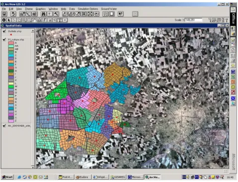
The application was improved with the Assign Proximity tool which analyses together a polygons theme and a points theme, and assigns to each polygon an attribute associated with the closest point, e.g., it is possible to know for each parcel which is the nearest water outlet. The figure2
represent the result of the Assign Proximity tool application in which was used the crop fields theme and a (draft) outlets theme. The different colors could represent the irrigation sectors in the real world.
Fig. 2 – Results map of the application of the Assign Proximity tool to identify the nearest outlet.
3.4 Application interface
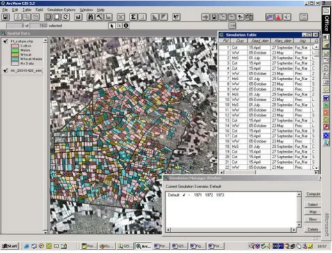
The main window for GISAREG application is composed of three areas (figure3) : one for map-ping, including the legend ; another for the simulation table described above or for presentation of results in table format ; and another for scenarios management (below at right). In addition to the ArcView’s default commands, there are several contextual menus, buttons and tools that where built to ease data input, building scenarios, and commanding the simulation operations and chart outputs. In the example of figure 3, the user has created the scenario “Default” and performed a simulation relative to the years 1971 through 1973. The same figure includes on the top left the contextual menu “Simulations options”, and on the top rights the buttons and tools for scenario editing and chart presentation.
The definition of irrigation options and water availability restrictions to be considered for si-mulation purposes are achieved through auxiliary windows. Irrigation scheduling options refer to the definition of soil water thresholds equal or below the optimal one, which is defined for the depletion fraction for no stress p (est-ce bien cela ?) (Allen et al., 1998), and the selection of irrigation depths. These may be defined as the amount of water required to refill the root zone storage up to the total available soil water (TAW) or to a percentage of TAW, as well as to adopt fixed irrigation depths (D) in relation to the irrigation method used. In the example in figure4a, the user created an irrigation option coded “Esq1” relative to fixed application depth D = 40 mm and irrigation timings when the soil water threshold at the four crop growth stages is 50% below the optimal ones.
The water restrictions apply to selected time periods and refer to a minimum interval between two successive irrigations or to the total water depth that may be used for irrigation during a given time interval. In the example of figure 4b, the water restriction coded “Res Cot” imposes a time interval between irrigations >15 days from 10 August to 30 September. Different water restrictions and irrigation scheduling options may be assigned to selected fields, crop systems or cropped areas through the simulation table.
observed by editing the “crop” column of the ST, or through a specific window as shown in Figure 5. The later helps the user to randomly assign the crop systems within the project area according some user-defined coverage percentages.
Fig. 3 – General view of the GISAREG application interface including the crops map and respective legend, the simulation table (ST) and the scenarios management window (below on right). On top left, the simulation options menu and, on top right, buttons and tools for scenario editing and chart outputs.
The spatial distribution of the crop systems may be submitted to restrictions on the use of some soil type for a given a crop system. A map is then created showing the spatial distribution of the crop systems that satisfy the user-defined criteria (figure5), which may be later imported to the ST and be used for a simulation scenario. The simulation of multiple scenarios allows visualizing the impacts of assigned irrigation management characteristics on water use and productivity, thus selecting the best alternatives for further implementation.
3.5 Outputs
GISAREG outputs can be presented in tabular, graphical (figures7and 7) or mapping formats and may concern a single field, the fields inside a selected area or the total area under study. In addition, results may refer to a single date, e.g. crop water deficits at a selected day, or the total simulation period, e.g. the crop irrigation requirements relative to a certain scenario. Annual results are stored in a ‘*.dbf’ table that has the same name as the simulation scena-rio followed by the simulation year. For any simulation scenascena-rio, there will be as many results tables (RT) as many years the user decided to simulate. The results table includes the infor-mation about : crops, crop irrigation requirements, available soil water at the beginning and at the end of the irrigation period, percolation, effective and non-used precipitation, groundwater contribution, potential and actual evapotranspiration, relative yield loss, critical unit flow rate and the monthly irrigation requirements.
Selecting the appropriate area on the map or the respective crop fields records in the simulation table, area aggregated results may be computed and displayed. The case in figure7concerns the
Fig. 4 – GISAREG forms for the definition of irrigation options (left) and water restrictions (right).
Fig. 5 – Windows for building simulation scenarios relative to crop selection, percentage of soil covered by a given crop, restrictions imposed on soil type relative to a given crop system, and mapping of the crop systems assigned to each field in the selected scenario applied to Gafura Gulyama area.
Fig. 6 – Simulation results presented as a map of crop irrigation requirements and water balance charts for two fields with different irrigation scheduling options, one for no stress, the other for water saving by allowing a controlled water stress.
computation of the demand hydrograph relative to a main node of the distribution system. The fact that the base remote sensing image is used in the GIS makes easier to identify the irrigation distribution network that concerns the area under analysis.
Fig. 7 – Irrigation demand hydrograph relative to the 1994 crop season for a selected node of the distribution system.
4
Application
GISAREG was applied to assess the crop irrigation requirements at Gafura Gulyama comparing different irrigation scenarios aiming at water savings (Fortes et al., 2003). Simulations refer to the crop data observed in the year 1999 and scenarios are the following :
– OY, aiming at attaining the optimal yield, adopting the p depletion fraction for no stress as irrigation threshold ;
– RES15, using the same irrigation threshold but imposing a 15 days time interval between successive irrigations (following the procedure described relative to figure 4b ;
– RES20, as above but with a time interval of 20 days ;
– STRESS, adopting a threshold 50% below that for OY (as described relative to figure
4a).
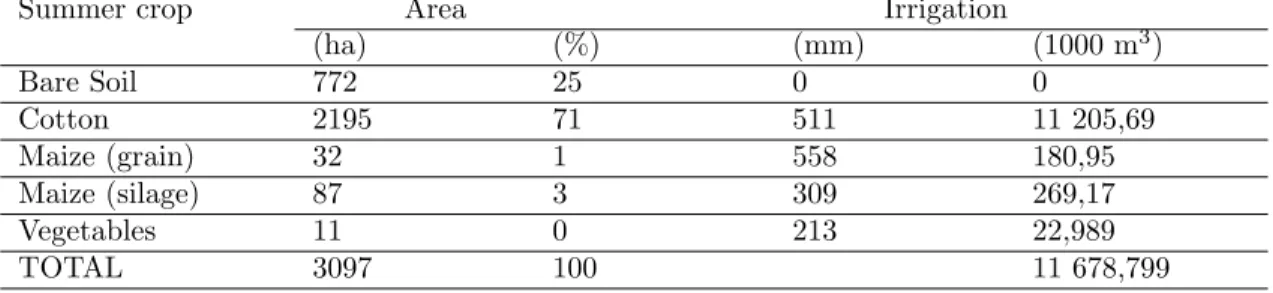
– Data in table 1 refers to the crop distribution pattern observed in 1999 and the cor-responding net irrigation requirements. The highest demand was from the grain maize (558 mm) followed by cotton (511 mm).
Tab. 1 – Observed crop pattern and net irrigation requirements for 1999.
Summer crop Area Irrigation
(ha) (%) (mm) (1000 m3) Bare Soil 772 25 0 0 Cotton 2195 71 511 11 205,69 Maize (grain) 32 1 558 180,95 Maize (silage) 87 3 309 269,17 Vegetables 11 0 213 22,989 TOTAL 3097 100 11 678,799
Simulation results are presented in Table 2 relative to the four scenarios. Results indicate that a water saving representing 9% of the irrigation demand with OY is attainable when adopting RES15, with relative yield losses of 7,3% in the cotton crop but above 17% for grain maize. The RES20 scenario produces 14% water savings but the relative yield losses increase to 11.5% for the cotton crop and >30% for the grain maize. The STRESS scenario leads to very high water savings, 3,4 million m3, i.e. 31% relative to OY. Consequently, it seems that the scenario STRESS could only be considered in case of severe restrictions on water supply because yield losses are high and would be of difficult application when salinity has to be controlled, as it is the case in the area. The scenarios RES15 and RES20 are generally feasible and allow for appropriate application of controlled leaching fractions with every irrigation event. However, RES20 is questionable for maize.
Tab. 2 – Comparing crop irrigation requirements I (m3) and relative yield losses Qy (%) referring to several irrigation scheduling scenarios aiming at water saving.
Summer crops Simulation scenarios
OY RES15 RES20 STRESS
I Qy I Qy I Qy I Qy (1000m3) (%) (1000m3) (%) (1000m3) (%) (1000m3) (%) Cotton 10596,166 2.0 9696,851 7,3 9192,325 11,5 7362,381 21,8 Maize (silage) 279,549 0 248,062 8,3 203,927 20,5 163,281 34,9 Vegetables 22,406 0.1 21,456 2.7 18,380 8,1 9,929 35,0 Total 11078,326 - 10121,182 9535,493 7642,216 Water saving 957,144 1542,833 3436,110 relativeto OY (8,6%) (13,9%) (31%)
Adopting RES15 produces an appreciable reduction in the demand volumes during the peak months of July and August. For July, the demand could reduce from 4 to 3,45 million m3 (13,8%), and for August it could decrease from 4 to 3,3 million m3 (17,8%).
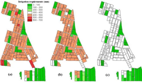
The results of the simulations for the scenarios OY, RES20 and STRESS referred above but applied to the average demand year are shown in 8. When visualizing such results it becomes apparent that a water saving of 13,9% in the seasonal demand is effectively important for only those crops having higher demand, maize in this application. On the contrary, when the STRESS scenario is adopted, it is well evident that it impacts most of the field crops.
Fig. 8 – Mapping crop irrigation requirements for the average demand year adopting three irrigation scheduling scenarios : a) OY, without water restrictions, b) RES20, for 20 days minimum interval between irrigations, and c) STRESS, adopting a low irrigation threshold.
GISAREG was also applied to assess the inter-annual variation of crop irrigation requirements. With this purpose, the model was run for all the years of the climatic data set and the wet, dry and average demand years were identified. Using the OY scenario, the season irrigation requirements for the wet and the dry year are compared through the GIS maps in9. They show that differences generally do not exceed 100 mm and they are apparent only for the cotton crop.
5
Conclusions
The integration of KCISA and ISAREG with the GIS ArcView 3.2 allows the easy handling of an irrigation scheduling simulation model over a large area or irrigation project, as well as the visualization of the spatial distribution of water demand inside that case study region or project. It is a useful tool for performing a large number of irrigation scheduling simulations, including for comparing different scenarios aiming at irrigation water savings. These capabilities were tested for an irrigated area in the Syrdarya basin, Uzbekistan. At present, this GIS application is being improved to be entirely applied in the Azizbek farm area, Fergana Valley.
The possibility for easily creating and changing scenarios allows the consideration of multiple alternatives for irrigation scheduling, including the adoption of crop specific irrigation mana-gement options. Scenarios may include different irrigation scheduling options inside the same project area applied to selected fields, crops, or sub-areas corresponding to irrigation sectors. This allows tailoring irrigation management according to identified requirements. Using the vi-sualization capabilities of GISAREG, it becomes easy to localize where discrepancies in water management may occur and how large they are, so providing criteria for technical intervention at field and project scales to improve water management.
It also allows an easy analysis of crop water and irrigation requirements and their spatial dis-tribution, thus to compare optimized/target demand with actual values. Such analysis may be performed at field scale, aggregated for a given area such as for computing a demand hydrograph at the nodes of an irrigation network, or for the entire project area. The case study presented herein shows good perspectives for the use of GISAREG to support irrigation management im-provements at both the farm and system scales that may lead to water saving and control of irrigation factors that favor desertification in the area.
R´
ef´
erences
[1] Allen R.G., Pereira, L.S., Raes D., Smith M., 1998. Crop Evapotranspiration. Guidelines for Computing Crop Water Requirements. FAO Irrig. Drain. Pap. 56, FAO, Rome, Italy, 300 p. [2] Campos A.A., Pereira L.S., Gon¸calves J.M., Fabi˜ao M.S., Liu Y., Li Y.N., Mao Z., Dong B., 2003. Water saving in the Yellow River Basin, China. 1. Irrigation demand scheduling. Agricultural Engineering International Vol. V (www.cigr-ejournal.tamu.edu).
[3] Doorenbos J., Pruitt W.G., 1977. Crop Water Requirements. Irrig. Drain. Paper 24, FAO, Rome, Italy, 193 p.
[4] Fernando R.M., Pereira L.S., Liu Y., 2001. Simulation of capillary rise and deep percola-tion with ISAREG. In : Wang M.H., Han L.J., Lei T.W., Wang B.J. (Eds.) Internapercola-tional Conference on Agricultural Science and Technology, Vol. 6 : Information Technology for Agriculture, ICAST, Ministry of Science and Technology, Beijing, China, pp. 447-455. [5] Fortes P.S., Pereira L.S., Rodrigues P.N., Calejo M.J., Teixeira J.L. and Platonov A.E. 2003.
GISAREG - A GIS Based Irrigation Scheduling Simulation Model to Support Improved Water Use and Environmental Control. In : Tarjuelo J.M., de Santa Olalla F.M. and Pereira L.S. (Eds.) Envirowater 2003. Land and Water Use Planning and Management (Proc. 6th Inter-Regional Conf. Environment-Water, Albacete, Sep. 2003), CREA, Univ. Castilla-La Mancha, Albacete, paper C-091 in CD-ROM.
[6] Liu Y., Teixeira J.L., Zhang H.J., Pereira L.S., 1998. Model validation and crop coefficients for irrigation scheduling in the North China Plain. Agri. Water Manag. 36 : 233-246. [7] Oweis T., Rodrigues P.N., Pereira L.S., 2003. Simulation of supplemental irrigation strategies
L.S., Oweis T., Shatanawi M., Zairi A. (Eds.) Tools for Drought Mitigation in Mediterranean Regions. Kluwer, Dordrecht, pp. 259-272.
[8] Pereira L.S., Teodoro P.R., Rodrigues P.N., Teixeira J.L., 2003. Irrigation scheduling simula-tion : the model ISAREG. In : Rossi G., Cancelliere A., Pereira L.S., Oweis T., Shatanawi M., Zairi A. (Eds.) Tools for Drought Mitigation in Mediterranean Regions. Kluwer, Dordrecht, pp. 161-180.
[9] Rodrigues P.N., Pereira L.S., Machado T.G., 2000. KCISA, a program to compute averaged crop coefficients. Application to field grown horticultural crops. In : Ferreira M.I., Jones H.G. (Eds.) Proceedings of the Third International Symposium on Irrigation of Horticultural Crops (Estoril, Jun-Jul 1999), Acta Horticulturae No 537, ISHS, Leuven, pp. 535-542. [10] Stewart J.L., Hanks R.J., Danielson R.E., Jackson E.B., Pruitt, W.O., Franklin W.T., Riley
J.P., Hagan R.M., 1977. Optimizing crop production through control of water and salinity levels in the soil. Utah Water Res. Lab. Rep. PRWG151-1, Utah St. Univ., Logan.
[11] Teixeira J.L., Pereira L.S., 1992. ISAREG, an irrigation scheduling model. ICID Bulletin, 41(2) : 29-48.
[12] Teixeira J.L., Paulo A.M., Pereira L.S., 1996. Simulation of irrigation demand at sector level. Irrigation and Drainage Systems, 10 : 159-178.
[13] Zairi A., El Amami H., Slatni A., Pereira L.S., Rodrigues P.N., Machado T., 2003. Coping with drought : deficit irrigation strategies for cereals and field horticultural crops in Central Tunisia. Rossi G., Cancelliere A., Pereira L.S., Oweis T., Shatanawi M., Zairi, A. (Eds.) Tools for Drought Mitigation in Mediterranean Regions. Kluwer, Dordrecht, pp. 181-201.