Publisher’s version / Version de l'éditeur:
Proceedings of the Ninth (1999) International Offshore and Polar Engineering
Conference, 2, pp. 622-627, 1999-05
READ THESE TERMS AND CONDITIONS CAREFULLY BEFORE USING THIS WEBSITE. https://nrc-publications.canada.ca/eng/copyright
Vous avez des questions? Nous pouvons vous aider. Pour communiquer directement avec un auteur, consultez la première page de la revue dans laquelle son article a été publié afin de trouver ses coordonnées. Si vous n’arrivez pas à les repérer, communiquez avec nous à [email protected].
Questions? Contact the NRC Publications Archive team at
[email protected]. If you wish to email the authors directly, please see the first page of the publication for their contact information.
NRC Publications Archive
Archives des publications du CNRC
This publication could be one of several versions: author’s original, accepted manuscript or the publisher’s version. / La version de cette publication peut être l’une des suivantes : la version prépublication de l’auteur, la version acceptée du manuscrit ou la version de l’éditeur.
Access and use of this website and the material on it are subject to the Terms and Conditions set forth at
Overview of a New Operational Model
Sayed, Mohamed; Carrieres, T.
https://publications-cnrc.canada.ca/fra/droits
L’accès à ce site Web et l’utilisation de son contenu sont assujettis aux conditions présentées dans le site
LISEZ CES CONDITIONS ATTENTIVEMENT AVANT D’UTILISER CE SITE WEB.
NRC Publications Record / Notice d'Archives des publications de CNRC:
https://nrc-publications.canada.ca/eng/view/object/?id=5b2aaea9-296d-4170-877b-c5363443d912
https://publications-cnrc.canada.ca/fra/voir/objet/?id=5b2aaea9-296d-4170-877b-c5363443d912
Proceedings of the Ninth (1999) International Offshore and Polar Engineering Conference Volume II, pp 622-627,
Brest, France, May 30-June 4, 1999
Overview of a New Operational Ice Model
Mohamed Sayed
Canadian Hydraulics Centre, National Research Centre, Ottawa, Canada
Tom Carrieres
Canadian Ice Service, Environment Canada, Ottawa, Canada
ABSTRACT
A new operational ice dynamics module has been implemented within the framework of the Canadian Community Ice-Ocean Model. The formulation is based on Hibler’s viscous plastic rheology, a Particle-In-Cell (PIC) approach to model ice advection, and a Zhang-Hibler scheme to solve the momentum equations. The PIC approach reduces numerical diffusion and improves the accuracy of predicting ice edge locations. Discretizing the ice cover into a large number of particles additionally simplifies modelling thickness distribution in great detail, without resorting to complex assumptions concerning a thickness distribution function. The Zhang-Hibler scheme leads to relatively high computational efficiency, and guarantees that the plastic yield conditions are satisfied. The program is tested using idealized cases, which demonstrate the model’s ability to predict ice edge locations, zones of high pressure, and ridging.
KEYWORDS: Sea ice forecasting, ice model, sea ice dynamics, ice drift, Particle-In-Cell, viscous plastic rheology.
INTRODUCTION
Ice dynamics models are routinely run to generate short-term products for all navigable waterways in Canada. Over the past few years, several requirements for improvements in the operational ice model have been identified. Those requirements include higher resolution, reduction of numerical diffusion particularly at ice edges, and improving the accuracy of predicting ice drift. This has prompted investigations concerning several aspects of the ice model such as ice cover rheology and various numerical formulations. Furthermore, a need has emerged for efficient means of sharing the results of ice model development, which take place at a number of agencies. Consequently, the Canadian Community Ice-Ocean Model (CIOM) has been developed as a framework for ice modelling research and operation. This paper reports on the development of a new ice dynamics module within CIOM. Early treatments of ice dynamics employed free-drift, linear viscous and elastic-plastic models. At present, however, most ice forecasting is based on the viscous plastic rheology and numerical formulation of Hibler (1979). The ice forecasting program presently used by the Canadian Ice Service is based on that model (a description was given
by Neralla, 1994). Other such operational models include PIPS (Posey and Preller, 1997).
An examination of different rheology models by Ip et al (1991) showed that shear strength is necessary for short-term forecasts. They also concluded that the elliptical yield envelope of Hibler (1979) provides the appropriate shear strength at low stresses. This contrasts with Mohr-Coulomb criterion, which corresponds to relatively small shear strength at low stresses. For long-term forecasts, however, the cavitating fluid model of Flato and Hibler (1992) was shown to provide appropriate accuracy, and additionally efficiency.
Discrete element models were also used in attempts to determine ice rheology. For example, Hopkins and Hibler (1991), and Sayed et al (1995) examined the deformations and stresses of assemblies of ice floes within rectangular test areas. The results of such studies, however, appear to depend on several factors concerning set-up of the problem, boundary conditions, and loading method. Therefore, they have not provided definitive conclusions regarding the appropriate shape of yield envelopes.
Numerical diffusion associated with finite difference solutions has been a source of inaccuracies, particularly in forecasting ice edge locations and high pressure zones. Flato (1993) developed a Particle-In-Cell (PIC) model, which improved the accuracy of predicting ice edge location. The PIC model is semi-Lagrangian. It is based on using discrete particles to model advection, while solving the momentum equations over an Eulerian grid. Other fully Lagrangian models have been developed including a discrete element model by Savage (1995) and a Smooth Particle Hydrodynamics by Gutfraind and Savage (1997). Those models greatly reduce numerical diffusion but the relatively high computational demand precludes them from operational use, at least at present.
As for solution of the momentum equations, Zhang and Hibler (1997) developed a semi-implicit finite difference method that appreciably improves efficiency. Their solution also guarantees that the yield criterion is satisfied through the use of pseudo time steps. Hunke and Dukowicz (1997) developed a different model based on an elastic-viscous-plastic rheology. That model reportedly leads to substantial improvements in computational efficiency.
The choice of modelling approach in the present work was aimed at meeting the requirements that were mentioned earlier, while adhering
to reliable methodologies. The main features of the model include the use of the viscous plastic rheology of Hibler (1979) since it is the most tested model and has been shown to suit short-term forecasting. The numerical solution of the momentum equations follows the method of Zhang and Hibler (1997) because of its efficiency, and in order to ensure that yield conditions are satisfied. A PIC approach (Flato, 1993) is used to model advection. Additionally, the PIC approach makes it possible to keep trach of thickness distribution in great detail, and in a simple manner. Huang and Savage (1998) showed that using PIC in conjunction with Zhang-Hibler numerical approach gives better resolution of ice edge locations than traditional finite difference formulation.
The following sections of the paper will discuss the governing equations and numerical solution method. Organiztion of the program and results of idealized test follow.
GOVERNING EQUATIONS Momentum and rheology equations
The ice cover is considered to move under the action of air and water drag, Coriolis force, and water surface tilt. Thus, the two-dimensional balance of linear momentum for a unit area of the ice cover is expressed as follows H hg u k hf dt u d h ice a w ice ice =∇
σ
−ρ
× +τ
+τ
+ρ
∇ρ
r r r r r . (1)where ρice is the ice density, h is the ice thickness,
u
r
is the velocity vector, σ is the stress tensor,
k
r
is the unit vector normal to the ice cover surface, f is Coriolis parameter, and
τ
ar
and
τ
wr
are the air and water drag stresses, respectively, g is the gravitational acceleration, and H is sea surface elevation. The air and water drag stresses are given by the following quadratic formulas
)
sin
cos
(
θ
θ
ρ
τ
ac
a aU
aU
ak
U
ar
r
r
r
r
×
+
=
(2) and(
)
(
)
[
β
β
]
ρ
τ
w cw w w u w u cos k w ur sin r r r r r r r − × + − = U - U U (3)where ca and cw are the air and wind drag coefficients,
U
ar
is wind velocity,
U
wr
is water velocity, β is the water turning angle, θ is the air turning angle, and ρa and ρw are the air and water densities,
respectively. Eq. (2) assumes that ice velocity is small compared to wind velocity. The turning angle, β is assumed to be the same for wind and water stresses.
A general form of the stress-strain rate relationship may be given by
ij kk ij ij ij
P
δ
ε
η
ζ
ε
η
δ
σ
=
−
+
2
•+
(
−
)
•2
(4) where • ijε
is the strain rate, P is the compressive strength as defined by Hibler (1979), and η and ζ are the shear and bulk viscosities, respectively. We note that P is different from the mean normal stress, which is commonly used in continuum mechanics literature. The compressive strength, P is usually considered to increase with increasing ice compactness, A (area of ice/total area). We use here the formula of Hibler (1979)[
(
1
)
]
exp
*A
C
h
P
P
=
ice−
−
(5)where P* is a reference ice strength, and C is a constant.
For small strain rates below a certain threshold, η and ζ are assumed to be constants and consequently the flow would be viscous. As strain rates exceed the threshold values, η and ζ can be chosen to represent a plastic yield envelope.
Hibler (1979) used an elliptic yield envelope and an associated flow rule to model the plastic regime. In that case the bulk and shear viscosities would be given by
2
2
e
P
ζ
η
ζ
=
∆
=
(6) where ∆ is given by(
)
− + + + + = ∆ • • − − • • • − • 0 2 2 22 2 11 2 12 2 2 2 22 2 11 )1 4 2 (1 ), ( max ε ε e e ε ε ε e ε (7) where • 11ε
, • 22ε
, and • 12ε
are the components of the strain rate tensor,• 0
ε
is the threshold strain rate, and e is the ratio between the major and minor axes of the elliptical yield envelope.Particle-In-Cell (PIC) advection
According to PIC formulation (Flato, 1993), the ice cover is discretized into individual particles that are advected in a Lagrangian manner. Each particle is considered to have an area and a thickness. For each time step, the particle velocities are determined by interpolating node velocities of an Eulerian grid. Particles can then be advected. The area and mass of all particles within each grid cell are then averaged to update the thickness and ice concentration at the Eulerian grid nodes. A bilinear interpolation function is used to map variables between the particles and the Eulerian grid. For a particle n at location xp, yp, and
grid node co-ordinates (xij, yij), the interpolation coefficients ω would
be given by
−
≤
∆
=
∆
−
−
∆
=
otherwise
x
x
t
n
x
if
n
j
i
S
x
n
j
i
S
x
t
n
x
x
t
n
x
x
ij p x x ij p p ij x0
)
,
(
1
)
,
,
(
)
,
,
(
|]
)
,
(
|
[
))
,
(
,
(
ω
(8) and
−
≤
∆
=
∆
−
−
∆
=
otherwise
y
y
t
n
y
if
n
j
i
S
y
n
j
i
Sy
y
t
n
y
y
t
n
x
x
ij p y ij p p ij y0
)
,
(
1
)
,
,
(
)
,
,
(
|]
)
,
(
|
[
))
,
(
,
(
ω
(9)where t is time, and ∆x and ∆y are the grid cell dimensions.
Thus, the particle velocity components, up and vp can be calculated as
follows ) , ( )) , ( , ( )) , ( , ( )) , ( ( ), , ( )) , ( , ( )) , ( , ( )) , ( ( j i v t n y y t n x x t n X v j i u t n y y t n x x t n X u p ij y p ij x j i p p ij y p ij x j i p ω ω ω ω ∑ ∑ = ∑ ∑ = (10)
where u(i,j) and v(i,j) are the velocity components of the Eulerian velocity grid.
Once particles’ velocities are determined, advection of a particle, n at location X, can be expressed as
∫
∆ +′
′
′
+
=
∆
+
t t tt
d
t
t
n
t
n
t
t
n
,
)
(
,
)
(
(
,
),
)
(
X
u
X
X
(11)where u is the particle’s velocity vector and ∆t is the time step. Following Flato (1993), the integral in Eq. (11) is approximated by
2
)
),
,
(
(
)
,
(
,
))
,
(
(
)
),
,
(
(
t
t
t
n
t
n
t
t
n
t
d
t
t
n
t t t∆
+
=
∆
=
′
′
′
∫
∆ +X
u
X
X
X
u
X
u
* * (12)The updated thickness and concentration are determined at each time step by mapping particles’ areas and volumes back to the Eulerian grid. In the present case, as will be discussed later, a staggered B-grid is used. Therefore the thickness and concentration values correspond to a set of nodes different from those used for the velocities. The values of node concentration c(xij, t) are determined as follows
∑
∆ ∆ = n ij y ij x ij y x t n A t n x t n x t x c( , ) ω ( ,X( , ))ω ( ,X( , )) ( , ) 1 (13)where A(n,t) is the area of particle n. The values of node thickness are then calculated as follows
∑
∆∆ = n ij ij y ij x ij y x t x c t n V t n x t n x t x h ) , ( 1 ) , ( )) , ( , ( )) , ( , ( ) , ( ω X ω X (14)where V(n,t) is the volume of particle n.
The resulting concentration and thickness are further modified to account for ridging, which may occur if ice converges. If the concentration at a node, according to Eq. (13), is larger than unity, its value is adjusted to one. The thickness at that node is also increased to conserve the volume of ice. The correction of concentration is mapped back to the particles. A factor F (larger than or equal to1) is used to reduce the area of each particle. Note that the volume of each particle is
conserved. Thus, the thickness of a particle is increased by the factor F. The value of F is determined by
{
( , ),1}
max ) , ( ~ 1 ), , ( ~ )) , ( , ( )) , ( , ( max ) , ( t x c t x c t x c t n x t n x t n F ij ij ij ij y ij x j i = ∑∑ = ω X ω X (15)THE NUMERICAL APPROACH
The solution is implemented using a staggered B-grid. The velocity components are defined at the corners of the velocity grid. All scalar values (pressure, viscosities, thickness and concentration) are defined at the centres of the grid cells.
Starting from a given initial configuration, the numerical solution of the above governing equations updates the velocities, pressures, thicknesses and concentrations at each time step. The main logic of the solution consists of the following steps:
• Advect the particles to new positions using Eqs. (11) and (12).
• Determine the thickness and concentration values by interpolating the area and volume of the particles to the scalar grid, according to Eqs. (13) and (14).
• Correct the thickness and concentration values by adjusting concentrations higher than unity. Next correct the area and thickness of each particle with the aid of Eq. (15).
• Calculate the pressures on the scalar grid using Eq. (5).
• Solve the momentum equations on the velocity grid. This is the major part of the solution, and is discussed below.
• Determine particle velocities by interpolating values from the velocity grid using Eq. (10).
Solution of the momentum equations follows the approach of Zhang and Hibler (1997). The solution steps may be summarized as follows. The momentum equations are arranged, with some terms to be treated implicitly, and others to be treated explicitly. A modified Euler time-stepping scheme is then used to solve the momentum equations in two levels. In the first level, the viscosity coefficients and diagonal water drag terms are considered to be functions of the previous time step. In the second level, those terms are evaluated using velocities at the centre of the time step. In those two levels, the off-diagonal water drag and Coriolis force terms are treated explicitly. Therefore, a third level correction is carried out in order to treat those terms implicitly. That correction produces a stable solution, with no strict limitations on the time step. The first and second level solutions can be done using either line relaxation or point relaxation. Although Zhang and Hibler (1997) indicate that line relaxation is more efficient, point relaxation is simpler and is used here in order to enhance simplicity and maintainability of the program. The preceding solution steps do not guarantee that the plastic yield condition is satisfied. In order to ensure that all stresses lie within the yield envelope, Zhang and Hibler introduced an additional pseudo time step iteration loop. This loop can be restricted to the second level solution, and corresponds to adjusting the viscosity coefficients each pseudo time step. The preceding discussion gives an outline of the solution method. Details of that method were given by Zhang and Hibler (1997).
Boundary Conditions
Land boundaries are introduced to the program via a mask, which assigns a value of 0 or 1 to cell centres (or thickness nodes). A value of 0 corresponds to land. All velocity nodes surrounding a land mask value of 0 are considered to have zero velocities; i.e. a no-slip condition is used at land boundaries.
The edge of the ice cover requires a more complex treatment, since its location changes throughout the solution steps. A velocity node is considered to correspond to open-water, when ice thickness (averaged from the 4 surrounding cell centres) is smaller than a minimum value (e.g. 0.05 m). For open water nodes, the momentum equations are solved as usual, but using a minimum value for ice thickness. Such a minimum value is needed to avoid divisions by zero. This procedure is commonly used to produce a continuous velocity field at the ice edge (Flato, 1998). Tests of the present program showed that this procedure gives more realistic results than those obtained by setting the velocities to zeros at open-water nodes.
At the outflow boundaries of the grid, a mask is used to assign zero values to cell centres. The corresponding values of the pressure and viscosity coefficients are set to zeros. Velocity nodes outside the outflow boundary are assigned zero values.
PROGRAM ORGANIZATION
The Community Ice-Ocean Model
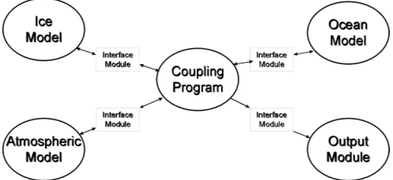
The CIOM is a framework for implementation of ice forecasting models. It is aimed at facilitating sharing of new developments and handling various input data formats. The approach of CIOM is based on encapsulating the various components of ice-ocean models in modules with standard interfaces. Thus modules can be shared and exchanged with relatively small effort. The framework of CIOM, as illustrated in Fig. 1, consists of an Ice Module, Ocean Module, and an Atmosphere Module. Those modules are connected via a Control Program. The data are defined in a Master Data Structure.
Fig. 1: Schematic diagram of the Community Ice-Ocean Model. The exchange of data takes place through interface modules: Ice Interface Module, Ocean Interface Module, and Atmosphere Interface Module. Each module also has its local variables. The values stored in the Master Data Structure are copied back and forth each time a module (e.g. the Ice Module) is called. Coding of the interface modules was developed by Chave and Fissel (1996). The Control Program directs intitialization, scheduling and time stepping. The Control Program also connects to utility modules that handle some input and output
operations. The interface modules allow off-the-shelf model components to be coupled with minimal code restructuring. The design also enables inter-model data exchange on different grids. The output module provides a uniform file structure for analysis and visualization of the results.
Outline of the Ice Module
The new Ice Module consists of a number of subroutines, which initialize and solve the dynamics equations. The initialization subroutine, is called only once at the start of a run. The first 3 subroutines read the input files (including land mask, ice chart and Ice Module parameters). After reading the input, a subroutine is called to place particles in each grid cell and to initialize the area and thickness of each particle. Two more subroutines are next called to calculate the pressure for each grid cell, and to map the velocities from the velocity grid to the particles. The steps of program initialization are summarized as follows:
• Read ice data. This consists of area concentration and thickness of each category (1 to 10), and for each grid cell. Initial velocities are assigned to the velocity grid.
• Initialize particle information. For each cell, the number of particles belonging to each category is determined, particles are placed within the cell, and a thickness and area are assigned to each particle.
• Pressure is calculated for each cell.
• Velocities are mapped from the velocity grid to particles.
The dynamics is called at each time step, with updated wind, ocean and thermodynamics variables. The main steps follow the above discussion of the numerical approach.
IDEALIZED TEST CASES
Operation of the program is examined in this section by considering two cases of idealized geometry and environmental forcing. An initial ice cover of 0.5 m thickness and 0.95 concentration is assumed to cover an area of 80 km by 100 km, with a land boundary at the east side. The grid consists of 10 km square cells, with 50 particles per cell. The initial positions of the particles are shown in Fig. 2. The ice cover is subjected to a constant uniform wind with a westerly component of 3.5 m/s and a southerly component of 6 m/s. The water current is assumed to be zero. The values of other run parameters are:
time step 30 minutes
mean latitude (for calculating Coriolis parameter) 35 degrees
air drag coefficient 0.003
water drag coefficient 0.005
turning angles (both air and water) 0
ice strength, P* 104 Pa
Elliptical yield envelope axes ratio, e 2
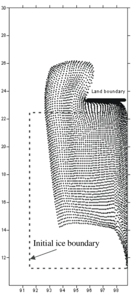
The resulting particle positions after 50 hours are shown in Fig 2. The resulting thickness, concentration, and velocity distributions are shown in Fig 3. A second test case was carried out using similar conditions to case 1, but also adding a land boundary at the northeast. The resulting particle positions are shown in Fig. 4.
The present results predict reasonable trends. The magnitude of predicted velocities and drift rates are in accordance with those of free
drift. The differences appear to correspond to the expected effects of land boundaries and the resulting internal ice pressure.
6 m/s
3.5 m/s
WIND
Land boundary
Fig. 2: Initial particle positions for the test cases.
Initial ice boundary
Fig. 3a: Particle positions after 50 hours (node numbers are shown
Fig. 3b: Pressure (P) distribution after 50 hours.
Fig. 3c: Thickness distribution after 50 hours.
CONCLUSIONS
A new Ice Module has been implemented within the framework of the Canadian Community Ice-Ocean Model (CIOM). The program includes two significant features, which meet previously established model requirements. The first feature is the use of a PIC scheme for ice advection. This reduces numerical diffusion, and particularly improves the accuracy of predicting ice edge locations. Discretizing the ice cover into a large number of particles has additional advantages. For example, thickness distribution is represented at great detail without resorting to arbitrary assumptions concerning a thickness distribution function.
The second main feature of the program is the use of the Zhang-Hibler numerical method to solve the momentum equations. That method leads to substantial improvements in the computational efficiency. Additionally, through the use of pseudo time steps, it guarantees that plastic yield conditions are satisfied.
Hibler’s viscous-plastic rheology is used in the present program since it is the most tested and accepted model. That rheology gives the ice cover a shear resistance, which is needed for the length and time scale
of interest. The Ice Module can be extended to include other plastic yield conditions such as the Mohr-Coulomb criterion.
The program was tested using idealized cases. Further testing using observations from the Gulf of St. Lawrence are currently underway.
Initial ice boundary
Fig. 4: Particle positions after 50 hours, north land barrier introduced.
ACKNOWLEDGEMENTS
The authors would like to thank S.B. Savage for valuable suggestions throughout the study. The financial support of the Program on Energy Research and Technology (PERD) is gratefully acknowledged.
REFERENCES
Chave, R and Fissel, D (1996). “Development of a control module for the Ice Ocean Community Model: implementation (draft version),” ASL Environmental Sciences Inc., Sidney, British Columbia, prepared for Ice Centre, Environment Canada, Ottawa, Ontario, March 1996. Flato, GM, and Hibler, WDIII (1992).”Modelling pack ice as a cavitating fluid,” J of Physical Oceanography, Vol. 22, pp. 626-650.
Flato, GM (1993). “A Particle-In-Cell sea-ice model,” Atmosphere-Ocean, Vol. 31, No. 3, pp. 339-358.
Flato, GM (1998). Personal communications.
Gutfraind, R, and Savage, SB (1997). “Marginal ice zone rheology: comparison of results from continuum-plastic models and discrete-particle simulations,” J. of Geophysical Research, Vol. 102, No. C6, pp.12 647-12 661.
Hibler, WDIII (1979). “A dynamic thermodynamic sea ice model,” J. Physical Oceanography, Vol. 9, No. 4, pp. 815-846.
Hopkins, MA, and Hibler, WD III (1991). “Numerical simulation of a compact convergent system of ice floes,” Annals of Glaciology, Vol. 15, pp.26-30.
Huang, ZJ and Savage, SB (1998).“Particle-In-Cell and finite difference approaches for the study of marginal ice zone problems,” Cold Regions Science and Technology, Vol. 26, No 1, pp 1-28. Hunke, EC, and Dukowicz, JK (1997).“An elastic-viscous-plastic model for sea ice dynamics”, J. Physical Oceanography, Vol. 27, No. 4, pp. 1849-1867.
Ip, CF, Hibler, WD III, and Flato, GM (1991). “On the effect of rheology on seasonal ice forecasting,” Annals of Glaciology, Vol. 15, pp.17-25.
Neralla, VR (1994). “Operational ice model at the Atmospheric Environment Service, Canada,” Proc. 4th Int. Offshore and Polar Engineering Conference, Vol. 2, pp. 473-478, Osaka, Japan, April 10-15.
Posey, PG, Preller, RH (1967).“The Polar Ice Prediction System (PIPS 2.0)-the Navy’s sea ice forecasting system,” Proc. 7th Int. Offshore and Polar Engineering Conference, Vol. 2, pp. 537-543, Honolulu, USA, May 25-30.
Savage, SB (1995).“Marginal ice zone dynamics modeled by computer simulations involving floe collisions,” in Mobile Particulate Systems, eds. E. Guazzelli and L. Oger, Kluwer Academic Publishers, pp. 305-330.
Sayed, M, Neralla, VR, and Savage, SB (1995).“Yield conditions of an assembly of discrete ice floes,” Proc. 5th Int. Offshore and Polar Engineering Conference, Vol. 2, pp. 330-335, The Hague, The Netherlands, June 11-16.
Sayed, M (1997).“Ice model development: review and work plan,” Technical Report HYD-TR-029, Canadian Hydraulics Centre, National Research Council, Ottawa, Ontario K1A 0R6.
Zhang, J and Hibler, WDIII (1997). “On an efficient numerical method for modelling sea ice dynamics,” J. Geophysical Research, Vol. 102, No. C4, pp. 8691-8702.