Channel coding for high speed links

(1)

Channel Coding for High Speed Links

by

Natasa Blitvic

B. Sc. A. Electrical Engineering, University of Ottawa, 2005

Submitted to the Department of Electrical Engineering and Computer Science in Partial Fulfillment of the Requirements for the Degree of

Master of Engineering in Electrical Engineering and Computer Science at the Massachusetts Institute of Technology

February, 2008

@2007

Author ... ...

Department of Electrical Engineering and Computer Science December 7, 2007

Certified by... ... ...

Vladimir Stoj ssista Professor f Electrical Engineering SM.I.T. _{Thesis Supervisor}

Accepted by... ... Terry P. Orlando

//" Terry P. Orlando Professor of Electrical Engineering Chairman, Department Committee on Graduate Theses

APR

0 7 2008

LIBRARIES

(2)

Channel Coding for High Speed Links by

Natasa Blitvic

B. Sc. A. Electrical Engineering, University of Ottawa, 2005

Submitted to the Department of Electrical Engineering and Computer Science in Partial Fulfillment of the Requirements for the Degree of

Master of Engineering in Electrical Engineering and Computer Science at the Massachusetts Institute of Technology

December, 2007

Abstract

This thesis explores the benefit of channel coding for high-speed backplane or chip-to-chip interconnects, referred to as the high-speed links. Although both power-constrained and bandwidth-limited, the high-speed links need to support data rates in the Gbps range at low error probabilities. Modeling the high-speed link as a com-munication system with noise and intersymbol interference (ISI), this work identifies three operating regimes based on the underlying dominant error mechanisms. The resulting framework is used to identify the conditions under which standard error control codes perform optimally, incur an impractically large overhead, or provide the optimal performance in the form of a single parity check code. For the regime where the standard error control codes are impractical, this thesis introduces low-complexity block codes, termed pattern-eliminating codes (PEC), which achieve a potentially large performance improvement over channels with residual ISI. The codes are systematic, require no decoding and allow for simple encoding. They can also be additionally endowed with a (0, n - 1) run-length-limiting property. The simulation results show that the simplest PEC can provide error-rate reductions of several orders of magnitude, even with rate penalty taken into account. It is also shown that channel conditioning, such as equalization, can have a large effect on the code performance and potentially large gains can be derived from optimizing the equalizer jointly with a pattern-eliminating code. Although the performance of a pattern-eliminating code is given by a closed-form expression, the channel memory and the low error rates of interest render accurate simulation of standard error-correcting codes impractical. This work proposes performance estimation techniques for coded high-speed links, based on the underlying regimes of operation. It also introduces an efficient algo-rithm for computing accurate marginal probability distributions of signals in a coded high-speed link.

Thesis Supervisor : Vladimir Stojanovic

(3)

Acknowledgement

The author would like to thank

Professor Vladimir Stojanovic, for his time, support, advice, and for painstakingly making her understand the meaning of practical. His breadth of knowledge and diversity of interests allowed this work on high-speed links to evolve in an admittedly unorthodox direction.

Professor Lizhong Zheng, for his dedicated interest in the project and enlivening discussions.

The Integrated Systems Group at MIT, for their friendship and skillful advice. In particular, the author is grateful to Maxine Lee, for paving the way; Ranko Sredojevic and Yan Li for their help with optimization; Fred Chen, Sanquan Song and Byungsub Kim for their knowledge of circuit design and high-speed links. This project did not have much in common with the work of Ajay Joshi, Ben Moss and Olivier Bichler, but what would life be without friends.

The author would also like to thank Her parents, for everything, and

(4)

2.2 Coding on ISI-and-AWGN-limited Systems - Symbol Error Probabilities 2.2.1 Symbol Error Probabilities in the Worst-case-dominant Regime 2.2.2 Symbol Error Probabilities in the Large-noise Regime ... 2.2.3 Symbol Error Probabilities in the Large-set-dominant Regime 2.3 Coding on ISI-and-AWGN-limited Systems - Joint Error Behavior

2.3.1 Joint Error Behavior in the Worst-case-dominant Regime . . 2.3.2 Joint Error Behavior in the Large-set-dominant Regime . . .

24 25

(5)

2.4 Codes for ISI-and-AWGN-limited Systems ... 54

2.4.1 Classical Error-Control Codes ... ... 54

2.4.2 Pattern-eliminating Codes ... . 55

2.4.3 Coding for High-speed Links ... ... 71

2.5 Practical Examples ... ... .. 75

2.5.1 Biasing the System Parameters ... 76

2.5.2 Code Performance in the Quasi-worst-case-dominant Regime . 77 2.5.3 Revisiting Previous Experimental Work . ... . 87

2.6 Summary ... ... .. 94

3 Performance Estimation of Coded High-speed Links 96 3.1 Preliminaries .... ... ... ... . . 97

3.1.1 System Model . ... ... .. . 97

3.2 Previous Work ... ... .. 99

3.3 Performance Estimation Methodology . ... 100

3.3.1 Computing the A Posteriori Signal Distributions ... . 101

3.3.2 Performance Estimation in the Worst-case-dominant Regime . 102 3.3.3 Further Use of Marginal Probability Distributions ... . 105

3.4 Efficient Computation of Probability Distributions for Coded Systems 105 3.4.1 Algorithm Description . ... ... 106

3.4.2 Generalizations and Remarks ... 117

3.5 Practical Examples ... ... 121 3.5.1 Runtime Statistics ... ... .. 122 3.5.2 Link Performance ... ... 123 3.6 Summary ... ... . ... 130 Conclusion 131 Appendix 134 References 139

(6)

Introduction

This thesis explores the benefit of channel coding for high-speed backplane or chip-to-chip interconnects, commonly referred to as the high-speed links. High-speed links are ubiquitous in modern computing and routing. In a personal computer, for instance, they link the central processing unit to the memory, while in backbone routers thou-sands of such links interface to the crossbar switch. Arising from the critical tasks they are designed to perform, high-speed links are subject to stringent throughput, accuracy and power consumption requirements. A typical high-speed link operates at a data rate on the order of 10 Gbps with error probability of approximately 10-15. Given the bandwidth-limited nature of the backplane communication channel, the ever-increasing demands in computing and routing speeds place a large burden on high-speed links. Specifically, high data rates exacerbate the inter-symbol interference (ISI), while the power constraints and the resulting complexity constraints limit the ability to combat the ISI. As a result, the system is no longer able to provide the required quality of communication. In fact, this residual ISI limits the achievable link data rates to an order of magnitude below their projected capacity [5].

Although most modern communication systems employ some form of coding as a technique to improve the quality of communication, the residual ISI severely im-pairs the performance of many such techniques. This is demonstrated in a thesis by M. Lee [4], which consists of a series of experimental results that evaluate the potential of standard error-correction and error-detection schemes for high-speed link applications. Moreover, coding schemes are also generally considered impractical for high-speed links due to the required overhead and the resulting rate penalty. Thus, most research efforts to bring more advanced communication techniques to high-speed

(7)

links have focused on improved signaling/modulation techniques and equalization [5, 16]. However, due to the previous lack of adequate theoretical and simulation frameworks, the previous conclusions regarding the benefit of coding for high-speed links are based on incomplete results and therefore remain speculative. Specifically, Monte-Carlo-based simulation techniques are not suitable for performance estimation of a coded high-speed link due to the low error probabilities, while the closed-form ex-pressions pertain to the limiting cases and may therefore not be sufficiently accurate. As a result, the most significant body of work on coding for high-speed links, [4], is purely experimental. The resulting practical constraints limit the depth of the analy-sis in [4] and further constrain the scope of the study to standard coding techniques, which may not be optimal in the high-speed link setting.

The present work addresses the issue of coding for high-speed links from a theoret-ical perspective, by abstracting the high-speed link as a general system with noise and ISI. This abstraction allows for a classification of possible error mechanisms, which enables both a deeper characterization of the behavior of different codes in a high-speed link and the development of new coding techniques adapted to these systems. The benefits of the regime classification also extend to system simulation, by allowing for more efficient simulation methods tailored for different regimes. In particular, this thesis develops the following results:

* A more complete characterization of error mechanisms occurring in a high-speed link. This enables the classification of system's operating conditions based on the dominant error mechanism as one of three possible regimes, namely, the large-noise, the worst-case-dominant and the large-set-dominant regimes. * A deeper characterization of codes for high-speed links. For instance, a

char-acterization of error mechanisms allows to identify the conditions under which standard error control codes incur little or no performance impairements due to the residual ISI. Note that these include, but are not limited to, the cases where the ISI is relatively weak compared to the noise.

(8)

* A new approach to coding under the worst-case-dominant regime where error is principally due to the occurrences of certain symbol patterns. The resulting codes, termed the pattern-eliminating codes provide the benefit of low complex-ity, allowing for simple encoding and requiring virtually no decoding.

* A theoretical framework for interpreting previously-documented experimental behaviors, such as [4] or [11, 12].

* New simulation methods for coded or uncoded high-speed links. The regime classification provides a more accurate guideline for biasing the system param-eters in simulation to capture error behaviors at low probabilities. Moreover, computational approaches that enable performance estimation without param-eter biasing are identified for each of the regimes.

* An efficient numerical algorithm for computing marginal probability distribu-tions in a coded system. The algorithm is of particular use under operating conditions that render the previous techniques impractical, either due to ex-cessive computational complexity or insufficient accuracy. Note that, since the performance of pattern-eliminating codes is given by a closed-form expression for all regimes of interest, the algorithm focuses on systematic linear block codes whose behavior is the focus of previous experimental work.

The three operating regimes are described qualitatively in Chapter 1 and quantita-tively in Chapter 2. The main body of results on coding for systems with noise and ISI, and the subsequent specialization to high-speed links, is contained in Chapter 2. The issue of system simulation for high-speed links is addressed in Chapter 3.

(9)

Chapter 1 The High-speed Link: The Reality

and the Abstraction

High-speed links typically refer to backplane or chip-to-chip interconnects that operate

at very high data rates (- 10 Gbps), low bit-error rate (~ 10-15) and with high energy efficiency. These stringent requirements arise from the critical tasks that high-speed links are designed to perform, as well as the global die-level and system-level power constraints. In a personal computer, for instance, they link the central processing unit to the memory, where ensuring an adequate speed and accuracy of the data transfer is essential. On a much larger scale, in backbone routers, thousands of such links interface to the crossbar switch. There, adequate accuracy guarantees the quality of the network traffic, the high speed reduces the number of links required to achieve the desired throughput, and high power efficiencies prevent that scaling from becoming prohibitive. In fact, the high-speed links form an integral part of many systems and their limitations thus generally have wide-ranging repercussions. This chapter begins by further describing the motivation behind the current high-speed-link research. Following the motivation, the high-speed high-speed-link is re-introduced in a more abstracted form: that of a communication system with inter-symbol interference (ISI) and additive white Gaussian noise (AWGN). The payoff of this abstraction is realized in the last section, which introduces three interference-and-noise scenarios that provide the foundation for the development of the subsequent chapters.

(10)

1.1 Motivation

The increasing demands in network and processing speeds have placed a large burden on high-speed links, as it is becoming increasingly difficult to keep up with the in-creasing data rates while maintaining the same reliability and adequately low power consumption. Referring again to the part played by high-speed links in backbone routers, [4] cites the following relevant example. Consider the result of using current technology to create a 40 Tb/s crossbar router chip. Since cross-bar router switches currently support 1 Tb/s, striving to reach the 40 Tb/s mark is a realistic goal. To achieve that throughput, 4000 of the current 10 Gb/s transceivers would have to be deployed. Since each transceiver uses a differential pair, the switch chip would need 8000 I/O pins, thus requiring the total on-chip area of 4000 mm2. The result-ing switch card would be roughly 4 meters (160 inches) wide and 2.5 meters (100 inches) long. Furthermore, since each transceiver currently dissipates 40 mW/Gb/s, the power consumption for the crossbar chip would total 1.6 kW, an unrealistically large number.

The above example illustrates the need for improved data rates and energy effi-ciencies of high-speed links. However, at higher data rates, the bandwidth-limited nature of the backplane as a communication channel coupled with signal reflections off of impedance discontinuities results in a large amount of inter-symbol interference (ISI). In these conditions, clever circuit design is insufficient to maintain adequate speed and reliability of the communication. Furthermore, the rate at which the communication channel degrades with the increasing data rates, coupled with tight power constraints, renders adequate' channel equalization impractical. The resulting uncompensated ISI, as further discussed in the following sections, becomes one of the dominant error mechanisms and limits the achievable link data rates to an order of magnitude below their projected capacity [5]. It is thus necessary to probe deeper into the communication theory and rediscover, or develop, more energy-efficient methods of ensuring adequate communication in these conditions. This thesis explores the

1

i.e. sufficient to achieve error rates on the order of 10

(11)

benefit of channel coding for high-speed links. In particular, it develops a new family of low-complexity codes, termed the pattern-eliminating codes, suitable in high-ISI regimes and provides a framework for simulation of standard error-control codes over channels with non-negligible ISI.

1.2 High-speed Link as a Communication System

The three principal error mechanisms in high-speed links, as described in [6] are in-terference, noise, and timing jitter. The interference in high-speed links is due to both the inter-symbol interference (ISI) and the crosstalk. The ISI is principally the result

of the dispersion, due to the fundamental loss mechanisms in the wire, including skin effect and dielectric loss, and the signal reflections off of impedance discontinuities. Crosstalk, which can also be considered as co-channel interference (CCI), is due to multiple signals traveling through the same backplane. The effects of both the ISI and the CCI on the received signal can be described through the convolution of the channel impulse response, sampled at symbol times, with the history of the transmit-ted symbols. Noise in high-speed links is typically small with respect to the signal magnitude. It is principally ascribed to thermal noise and transistor device noise, and is therefore modeled as additive, white and Gaussian (AWGN) with standard de-viation in the range of 3 mV down to 0.3 mV approximately, where the transmitted signal swing is + IV. The timing jitter is tied to the transmitter phase-locked loops (PLL) and the received clock data recovery (CDR) circuits. Various jitter models are available and many are overviewed in [6]. Since the ISI has been identified as the dominant error mechanism in a high-speed link [5], this thesis focuses on ISI-limited channels with AWGN.

The resulting simplified model of a typical high-speed link as a communication system is shown in Fig. 1-1. The system employs PAM2 modulation and the equivalent communication channel is discrete. The latter also includes the effects of any signal processing in the transmitter or the receiver, such as equalization or matched-filtering. Due to the practical limits of equalization in high-speed links, the equalized channel

(12)

Figure 1-1: Model of a High-speed link as a Communication System

response typically contains some amount of residual inter-symbol interference. Due to hardware complexity constraints, the detection scheme at the receiver is a blind application of the symbol-by-symbol maximum a posteriori (MAP) detection [3] for channels without ISI, rather than a more complex sequence detection scheme, such as [26], developed for channels with ISI.

Concerning notation, it is convenient to denote the received signal at some time index i as YI and represent it as the sum of a signal component Zi and the noise component Ni. Note that, throughout this thesis, upper-case notation is used to represent random variables, while the lower-case notation denotes the corresponding realizations and other deterministic quantities. The exception to this rule is the length of the channel response, denoted by L in order to be distinguished more easily from the ubiquitous time index i. Thus, for a channel of length L, the signal component

Zi is given as the sum of the current symbol and the L - 1 previously2 transmitted symbols, weighted by the channel coefficients. The value z such that when Z = z

the signal suffers no ISI is referred to as the signal mean, despite the fact that for constrained (coded) symbols z may not equal the expectation of the random variable

Zi.

Given a sequence of transmitted symbols Xi, .. , Xi-L+ E {--1, 1}, where Xi is transmitted last, and some equivalent channel response of length L specified by the coefficients ho, ... hL-1 E , the corresponding Y4 is given by

L-1

Yi = Xi-khk + N (1.1)

k=O

2In case the channel also causes precursor ISI, that is, has a non-causal impulse response, the

L - 1 interfering symbols also contain "future" symbols.

(13)

Since, Yi is discrete, its marginal probability distribution is specified by the prob-ability mass function (PMF), denoted by fyi, or alternatively, by the cumulative mass function (CMF), Fy,. For a communication channel with ISI, the dependen-cies between the received symbols resulting from the convolution equation (Eqn. 2.1) imply that the set of marginal distributions fy,..., fy,,_, is typically not sufficient to specify the joint distribution fy,...,Yi+L-1. However Chapter 2, among other re-sults, describes some special circumstances under which the joint and the marginal distributions are effectively interchangeable.

1.3 Classification of Error Mechanisms in

High-speed Links

Motivated by the model of a high-speed link introduced in the previous section, this section provides a more thorough characterization of the error mechanisms in systems limited by AWGN and ISI. Typically, the dominant error mechanism is loosely defined as the most likely source of detection errors. For instance, [6] observes that the inter-symbol interference, rather than noise alone or the timing jitter, is the dominant error mechanism in a high-speed link. In the present context, however, the term takes on a more precise meaning. Specifically, the dominant error mechanism refers to an

attribute of a set of interference events which are found to be responsible for some

large proportion of the detection errors.

The concept of a dominant error mechanism is formalized in Section 2.2 of Chap-ter 2. In the meanwhile, to gain a qualitative understanding of the concept, different error mechanisms are examined through the a posteriori probability distribution of the random variable Z , defined in the present context as the probability distribu-tion of Zi condidistribu-tioned on the occurrence of an error event. More precisely, letting

P(Zi = z) denote the a priori probability of observing some signal component z of

the total received signal, the corresponding unilateral a posteriori probabilities are given by P(Z, = z Yi < 0, X = 1) and P(Zi = z I Y > O,XX = -1). In a

(14)

loose sense, the a posteriori distribution specifies the proportion of the errors that are due to each possible interference event. However, several factors jointly determine the a posteriori probability distributions and different combinations of these factors give rise to distinct scenarios or regimes. Specifically, it is clear that in a communi-cation system with noise and ISI, the nature of the main error mechanism is some factor of the magnitude of the ISI relative to the transmitted symbol power, the noise variance relative to the transmitted symbol power, and the magnitude of the ISI rel-ative to the noise variance. A more precise characterization yields the following three noise-and-interference scenarios, which enable the classification of any communication system that is principally limited by noise and ISI. They consist of the large-noise

scenario, the worst-case-dominant scenario, and the large-set-dominant scenario. In

the large-noise scenario, ISI is negligible with respect to noise and the latter dom-inates the error expression, while the error in the worst-case-dominant scenario is principally attributable to the occurrence of symbol patterns causing worst-case in-terference. The large-set-dominant scenario encompasses the remaining conditions, but also allows for a general result regarding joint error behaviors. The corresponding classification framework is at the core of the results formulated in the later chapters, which develop both codes and simulation methodologies to suit particular regimes in a system with noise and ISI.

Prior to discussing individual scenarios, note that, from the theoretical perspec-tive, the three different scenarios represent three different limiting behaviors. This view is further discussed in Chapter 2. On the other hand, from a practical stand-point, the three scenarios provide a classification framework where the boundaries are context-dependent. For instance, regarding the performance of codes optimized for a given limiting behavior3_{, the boundary of the corresponding regime is set to}

encompass the operating conditions under which such codes provide a benefit. Sim-ilarly, from the point of view of performance estimation, it is convenient to consider as large-set dominant all conditions under which the error events can be considered

3

1In _{Chapter 2, standard error correction codes are shown to perform optimally in the limit of} the large noise regime and a subcase of the large-set-dominant regime, while the pattern-eliminating codes are developed for the limit of the worst-case-dominant regime.

(15)

as statistically independent, with some sufficient accuracy.

The following discussion pertains to an arbitrary real channel of length L whose smallest-magnitude coefficient is denoted by 6. The worst-case interference incurred by the signal, that is, the maximum deviation from the signal mean in either direction, is represented by some A > 0. In other words, letting z denote the corresponding signal mean4, the random variable Zi takes values from the interval [z - A, z + A]. Also, note that the worst-case interference is lower-bounded by (L - 1)6 and that possible values of Zi occur in increments of at least 26. The quantity cs I denotes

the variance of the ISI, that is, of the random variable Zi - hoXi. The noise (AWGN)

is assumed to be independent of the signal, with zero mean and some variance a2.

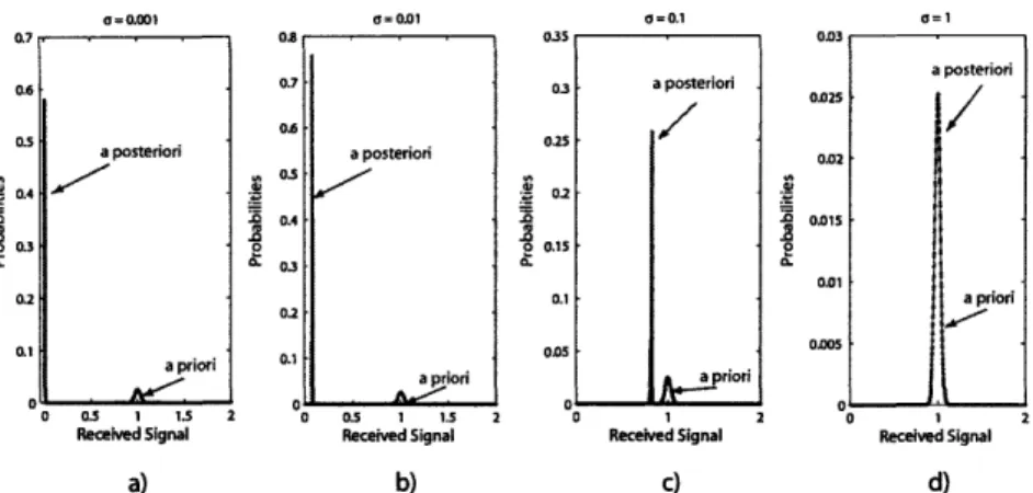
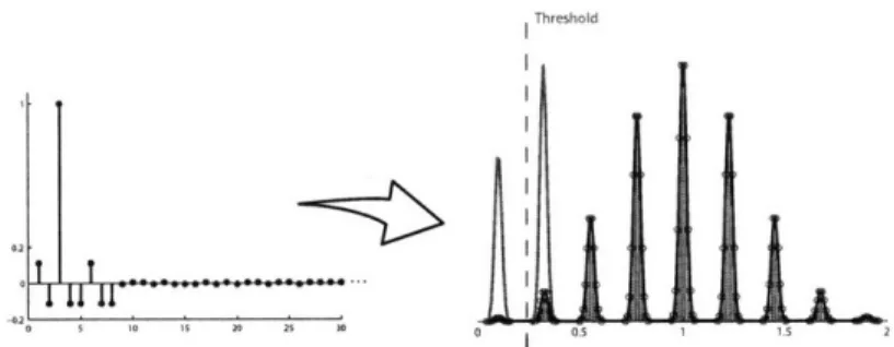
The two sets of plots of Figures 1-2 and 1-3, depicting the a posteriori probability distributions for the random variable Zi as a function of c and 6, are used in the sections that follow to exemplify and link the three scenarios. The probability dis-tributions are computed based on the decision threshold of zero, for a channel with

z = 1 and interference coefficients that take values from the set {-6, 6}, for some positive real 6. Different scenarios are obtained by controlling the value of 6 and a. For the purpose of illustration, it is also assumed that the symbol patterns are unconstrained. Thus, the a priori probabilities for the normalized interference, appro-priately shifted and scaled, follow a binomial distribution with p = 0.5. The changes in the behavior of the a posteriori probability distribution resulting from varying the channel and noise parameters are indicative of the shift in the error mechanism as the system transitions from one limiting case to another.

1.3.1 Large-noise Regime

The large-noise regime occurs when the noise variance a2 is sufficiently large relative to the variance of the ISI, ofsI. Then, conditioning on the signal variable Zi, in the

Yj = Z2 + Ni expression, provides little information about the received signal Yi and

the a posteriori symbol interference probabilities are approximately equal to the a

4

i.e. the value of the signal in the event that no ISI occurs. If the transmissions are coded, z may not equal the expectation of the random variable Zi.

(16)

.7 08 035 0.6 0.7 0.3 a posteriori 0.5 a posteriori a posteriori 0.25 0.5 0 O.4 0 0.2 0.2 0.1 0.2 . a priori .1 05 . a p iori I a prior 0 o0 D03 a posteriori 0.02S oD2 . 0,015 0005 0 _{a pior} ODOSn 0 0.5 1 1.5 2 0.5 1 2 1 2 0 1

Received Signal Received Signal Received Signal Received Signal

a) b) c) d)

Figure 1-2: A priori and a posteriori probability distributions for a channel of length L =

1000 varying noise levels - a) a = 0.001, b) a = 0.01, c) a = 0.1, d) a = 1. The system in a) operates in the worst-case-dominant regime, while d) operates in the large-noise regime. The remaining cases are large-set-dominant.

priori probabilities. The large-noise regime is illustrated in Figures 1-2 d) and 1-3 e) although, depending on the context, the setup of Figure 1-3d) could be considered large-noise as well. Note that as,2 = 10- 3 for the system of Figure 1-2 and a:s, = 0.1 for that of Figure 1-3.

The relative magnitudes of noise variance and the ISI required for the system to operate in the large-noise regime also depend on the signal mean z. For a system operating "far" from the decision threshold, a tolerable amount of ISI for the large-noise regime to apply is significantly lesser than that required for a system operating closer to the decision threshold. As an illustration, consider a system with noise of variance a2 and let 6 be the channel coefficient of smallest magnitude. If the system indeed operates in the large-noise regime, then the ratio of the a posteriori probabilities for two different ISI values will be equal to the ratio of their a priori probabilities. Now, let z be sufficiently large, so that any detection error is due to a low-probability noise event. Since cumulative probabilities in the tails of the Gaussian distribution can be approximated as

Sz2

P(N > z) . (1.2)

~ZV~ 1.2

(17)

0.9 0.8 0.7 S0.6 0 o.5 0.4 0.3 0.2 0.1 S= 0.01 C=0.1 0 0.5 1 1.5 2 0 0.5 1 1.5 2 0.5 1 1.5 2 0 2 1

Received Signal Received Signal Received Signal Received Signal Received Signal

a) b) c) d) e)

Figure 1-3: A priori and a posteriori probability distributions for a channel of length L = 10 varying noise levels - a) a = 0.001, b) a = 0.01, c) a = 0.1, d) a = 1, e) a = 4. Systems a) through c) are worst-case-dominant, while e) operates in the large-noise regime. System d) is large-set-dominant, but could be considered large-noise depending on the context.

obtained by truncating5 the corresponding asymptotic series [19], then, placing the decision threshold at zero, the ratio of the a posteriori probabilities between the signal incurring no ISI and that suffering interference of 26 in the direction of the decision threshold is given by P(Zj = zY < 0,X, = 1) P(Zi = z)P(Ni > z)

P(Zj = z - 261Y < O, X = 1)

P(Z, = z - 26)P(N, > z - 26)

z 2 P(Zi = z) (z - 26)e2T

P(Zi = z -

26)

ze

P(Zi = z) z - 26 -2z/u2+262/ 2 --

---P(Zj = z- 26)

z

As z gets larger, keeping 6 and a constant, the ratio (z - 26)/z tends to unity,

but the factor e-za/ " _{tends to zero and the ratio of the a priori probabilities is thus} not maintained. Thus, as z increases, the operating conditions move away from the

large-noise regime.

5_{The accuracy of both the asymptotic expansion and the subsequent truncation is discussed in}

Section 2.2.2 of Chapter 2.

a=0.001

0- _aý2 I Aj 2 .· e c 0

(18)

1.3.2 Worst-case-dominant Regime

The worst-case ISI occurs when a transmitted symbol pattern causes the received signal to deviate from its mean value z by the maximum possible amount A in the direction of the decision threshold. For a channel of length L defined by coefficients

ho, hi,..., hL-1, where hi,... , hL-1 cause interference, there are two possible

worst-case patterns, depending on the value of the most-recently transmitted symbol Xi:

(Xi,..., Xi-L+1) = (sign (ho), -sign (hi), -sign (h2),.. . , -sign (hL-1))

and

(Xi,... , Xi-L+1)= (-sign (ho), sign (hi), sign (h2),..., sign (hL-1))

The system effectively operates in the worst-case-dominant regime when both of the following two conditions are satisfied:

1. The signal value affected by the worst-case ISI is at some non-negative distance away from the decision threshold, i.e. the minimum decision distance is positive. 2. The noise standard deviation, u, is small relative to the channel coefficient of

least magnitude, 6.

Then, the error events are principally due to the occurrence of the worst-case ISI coupled with a noise event. The corresponding a posteriori probability distributions for the observed interference therefore assign some large probability to the worst-case event. This occurs in Figures 1-2 a) and 1-3 a- c). Note that the a posteriori probability in Figure 1-2 b) is not concentrated on the worst-case interference, but on some adjacent interference value. Thus, whether to categorize the corresponding regime as worst-case-dominant is context-dependent.

The positive distance by which the signal mean z is separated from the decision threshold affects the allowed range for the 6/a ratio. Applying the expression of Equation 1.2 for the cumulative probability in the tails of the Gaussian distribution, it follows that the allowed range for the values of 6/1 can be relaxed as the mean signal

(19)

value z moves away from the decision threshold. More precisely, the factor e-z l/" now serves to suppress the a posteriori probability of symbol patterns which do not bring the signal the closest to the error region. For large z where this expression is valid, increasing z by a factor of ac > 1 allows to reduce the 6/1 _{ratio roughly by a factor}

of 1/a.

However, for some given a, 6 and z, whether a system operates in the worst-case dominant regime is also a function of the channel length L. Since several symbol patterns can cause an identical amount of ISI, both the a priori, and therefore the a posteriori, signal probability distributions take into account this multiplicity. Thus for large L, the multiplicity can bias the a posteriori distributions away from the worst-case. As an illustration, comparing the individual plots of Figures 1-2 and 1-3 yields four pairs of systems with equal a and z, but different L. Although the 6 of the plots correponding to Figures 1-3 b-c) (L = 10) is greater than that of the systems in Figure 1-2 b -c) (L = 1000), the former operate in the worst-case-dominant regime while the latter do not.

Finally, it remains to justify the non-negativity requirement on the minimum decision distance. Placing once again the decision threshold at zero, assume that

z' = z - A < 0 where z' represents the value of the noiseless received signal Zi

when affected by the worst-case ISI. Suppose in addition that there exists another possible value of Zi, denoted by z", that is also at a negative distance from the decision threshold. More precisely, there exists some possible outcome z" such that

z' < z" < 0. Then, for sufficiently large L, conditioning on an error event may assign a larger a posteriori probability to z" than to z' simply on account of its multiplicity. An example of this occuring is depicted in Figures 1-4a)-c) below. In particular, for the system depicted in the part a) of the figure and operating in the worst-case-dominant regime, the signal mean z is reduced by 2.56 and 46 so that the worst-case interference crosses the decision threshold. The resulting a posteriori probability distributions, displayed in parts b) and c), are no longer worst-case-dominant, as the probability mass is centered on the interference values closer to the decision threshold. Alternatively, a more precise argument justifying the non-negativity requirement

(20)

is available when the noise variance is sufficiently small so that the probabilities

P(N < z') and P(N < z") are both from the tails of the Gaussian distribution. In

those conditions, the ratio of the a posteriori probabilities becomes: P(Zi = z'lY| < 0, Xi = 1) P(Z1 = z')P(Ni < -z')

P(Zj = z"1Y < O, Xi = 1) P(ZX = z")P(Ni < -z") P(Z% = z')P(Ni > z') P(Z, = z")P(Ni > z") P(Zi = z') z" 1 - e2 x -XX P (Zi = z") z' -e

Since

Iz'l

> _{Iz"j, the two ratios on the left-hand side are both less than unity. Thus,}

if z" has an equal or greater a priori probability than z', the a posteriori probability will be biased in its favor. The regime will therefore not be worst-case-dominant.

However, note that the non-negativity requirement on the minimum distance is in principle too strict. More precisely, it is possible to envision a case where z' is the only possible negative ISI value and the next-to-worst-case ISI is sufficiently removed for the above ratio to be large and for the error expression to remain dominated by the occurrence of the worst-case ISI. While this case may be of some practical importance, a simpler definition which encompasses a large number of cases is preferable for the purpose of the subsequent development.

Quasi-worst-case-dominant Scenarios

While the previous development concerns the regime where the worst-case interference is responsible for most of the error events, such a behavior is seldom observed in practice. Instead, a more common occurrence is that of a dichotomous channel. The term refers to any channel of length L whose i coefficients are more significant than the remaining ones. The notion of significance is context-dependent. For instance, it may pertain to the confidence of the channel response measurements, or, in dispersive channels, to the fact that the first 1 coefficients are typically of larger magnitude. In general, the corresponding 1 coefficients are referred to as the principal part of the

(21)

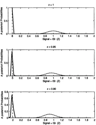
b 0.2 0.4 0.6 0.8 1 1.2 1.4 1.6 1.8 Signal+ ISI (Z) z = 0.95 5 0 - 0.2 0.4 0.6 0.8 1 1.2 1.4 1.6 1.8

A

Signal + ISI (Z) z=0.90 0 0.2 0.4 0.6 0.8 1 1.2 Signal + ISI (Z) 1.4 1.6 1.8 2

Figure 1-4: Illustrating the non-negative-minimum-distance requirement for the worst-case-dominant regime. In all three plots, a = 0.01, 6 = 0.02, L = 50 which implies that A = 1. The decision threshold is placed at zero as indicated by the dashed line, and the

corre-sponding minimum decision distance is given by z - A. The corresponding error probabil-ities Perr are included for completeness. - a)z = 1,perr = 4.5 x 10-16. The a posteriori probability of the case pattern is 0.9968, thus the regime can be considered worst-case-dominant for many practical contexts. b) z = 0.9 5,perr = 4.0 x 10-14. The symbol patterns that produce second-to-worst ISI have the largest a posteriori probability. c) z = 0.9 0,Perr = 1.5 x 10-12. The set of symbol patterns that causes the received symbol to fall into the region [-36, 36] dominates the a posteriori probabilities. The worst-case ISI, which causes the event Z = -56, is not part of this set.

Cu n S,02 IL0. 0 aO.CL U, 2 0.0 0 .1 "C 0.6 20 n 0.4 0.2 aS 0

-t'

<:

(22)

b I I---I

Respons majority

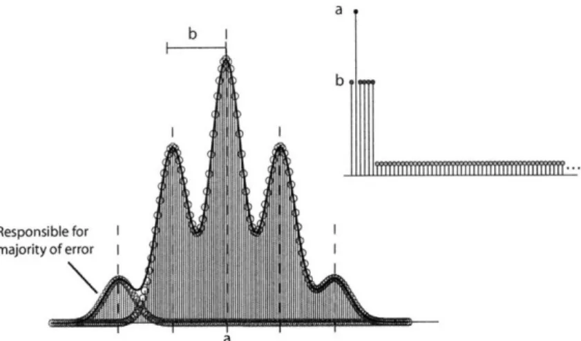
Figure 1-5: A Dichotomous Channel in the Quasi-worst-case-dominant Scenario Note that, in general, the I coefficients need not occur consecutively, nor be restricted to a specific portion of the channel.

By considering an equivalent channel of length 1, the previous characterization of the worst-case behaviors extends to worst-case interference caused by the principal part of the channel. The corresponding regime is referred to as the

quasi-worst-case-dominant regime and is illustrated in Figure 1-5 for a two-level channel. In this

example, the principal part of the channel has length 1 = 5, signal mean z = a and interference coefficients of magnitude b, while the secondary part of the channel has coefficients of some lesser, unspecified magnitude. The plot illustrates only the a

priori probability distribution of the random variable Zi and highlights the events

that aggregately dominate the a posteriori probability. The latter correspond to all the events associated with the worst-case patterns ±(-1, 1, -1, -1) formed by the principal part of the channel and producing signal values centered at a - 4b.

1.3.3 Large-set-dominant Regime

In the subsequent chapters, the large-set-dominant regime is principally considered as a default regime for all the cases that, in a given context, do not fit the two other regimes. For instance, it can be used to classify the behaviors illustrated in Figures 1-2a-b) and, depending on the context, 1-2c-d). It also applies to the

(23)

conditions of Figure 1-4, where the system does not operate in either the worst-case or quasi-worst-case-dominant regime due to the negative decision distance. Since the large-set-dominant scenario encompasses a range of possible a posteriori probability distributions, more general results regarding the error affecting any given symbol are difficult to formulate. Instead, Chapter 3 develops a numerical algorithm for computing probability distributions when a system cannot be considered to operate in one of the limiting cases.

However, an important general result regarding the large-set-dominant scenario can be formulated with respect to the joint error behaviors. Specifically, in large-set-dominant conditions that are sufficiently removed from the worst-case or quasi-worst-case scenarios, the error events on the received signals can be considered effectively in-dependent. Since the corresponding conditions pertain to joint error statistics, rather than the a posteriori error probabilities, these cases are discussed in Section 2.3.2 of Chapter 2.

1.4 Summary

The purpose of this chapter is two-fold. First, it seeks to convey the sense of ur-gency which permeates many aspects of the high-speed link research, in a race to keep up with the ever-increasing demands in speed and energy-efficiency. Second, it introduces an abstracted framework suitable for a more theoretical approach to high-speed links. Modeling a high-speed link as an ISI-limited system with additive white Gaussian noise, possible error mechanisms are categorized according to three scenarios, or regimes: the large-noise, the worst-case-dominant and the large-set-dominant. This categorization plays an important part in the subsequent chapters by providing means for a significantly more rigorous analysis than that achieved in the previous work on coded high-speed links, as well as enabling the development of new, alternative error-control methods tailored for the different scenarios.

(24)

Chapter 2 Coding for High-speed Links

Most modern communication systems employ some form of coding as a technique to improve the quality of communication. These often include redundancy-based error control codes that allow for error detection or correction, run-length-limiting codes that improve the receiver's clock recovery, or DC-balancing codes that protect the timing circuitry against capacitative coupling. While inter-symbol interference (ISI) has a limited effect on the timing properties of a code, the performance of error-control codes is significantly impaired, as demonstrated in [4]. A variety of higher-complexity techniques discussed in Section 2.1.3 combat the ISI to some extent, but few are suitable for power or complexity-constrained systems.

The developments in this chapter build on the regime classification framework de-veloped in Chapter 1 in order to further characterize the marginal and the joint error behaviors of systems with noise and inter-symbol interference. The corresponding re-sults provide conditions under which standard error-control codes perform optimally' and, otherwise, lead to a new approach to error-control coding for the worst-case-dominant or quasi-worst-case-worst-case-dominant regimes.

'That is, the conditions where the ISI has little effect on the joint error statistics and the error control suffers little or no impairement.

(25)

2.1 Preliminaries

This section overviews the basics of error-control coding and extends the previously-described high-speed link model to include coded transmissions. Previous work re-garding coding for high-speed links is overviewed as well.

2.1.1 Error-control Coding

This section briefly overviews the basic principles of error-control coding of use in Chapters 2 and 3. A more thorough treatement is available in [1] or [2].

Error-control codes codes introduce controlled redundancy in order to improve the reliability of the transmission, either through forward error correction or error cor-rection with retransmissions. Note that the corresponding stream of bits is therefore necessarily constrained. In an (n, k) binary linear block code, each n-bit codeword is

obtained through some linear combination, over the binary field F2 = {0, 1}, of the underlying k information bits. In a systematic linear block code, the k information bits appear explicitly, along with the n - k parity bits computed using a binary map.

Linear block codes over finite fields of higher orders operate on the same principle. The most celebrated example are the Reed-Solomon codes, which are extensively used in data storage and telecommunications.

Linear block codes are intuitively simple and thus commonly provide a starting point for new applications, as further discussed in Section 2.1.3. However, the concept of error-control coding also extends to the more powerful convolutional, LDPC and turbo codes.

Regarding decoding, a system can implement hard-decision decoding or soft-decision decoding. Hard-soft-decision decoding operates over a finite field and is thus decoupled from the detection problem. In soft-decision decoding, the real-valued sig-nals are used in order to make more informed decisions. Although hard-decision de-coding allows for relatively simple hardware implementations-for binary linear block codes, the setup is a simple threshold device folowed by delay and logic elements-the soft-decision decoding provides a performance benefit.

(26)

A notion of importance in linear block codes is that of Hamming distance. For any two codewords, the Hamming distance corresponds to the number of positions, out of

n, where the codewords differ. For some coodebook C, defined as the set of allowed

n-bit codewords, the minimum Hamming distance dH is defined as the minimum distance between any two codewords in the codebook. Assuming hard-decision decoding and correcting to the nearest2 _{codeword, a codeword will be decoded correctly if and only}

if there are less than [dH/2J detection errors in a codeword. The quantity LdH/2J is the error-correcting power of a code, denoted by the parameter t.

Note that in bandwidth-limited systems, an important factor of the code perfor-mance is the coding overhead. The coding overhead refers to the fact that only k bits out of the n codeword bits carry information. For a coded system operating at some signalling rate R, the equivalent information rate is thus Rk/n. When a system is severely bandwidth-limited, it can happen that an uncoded system operating at a rate of Rk/n can outperform a coded system operating at rate R. In the context of this thesis, this behavior is referred to as the rate penalty of a code.

2.1.2 System Model

The system model is that of the abstracted ISI-and-AWGN-limited system intro-duced in Chapter 1, with the addition of an encoder/decoder, as shown in Figure 2-1. Despite the fact that the depicted system implements hard-decision decoding, the de-velopments of Chapters 2 and 3 are general, unless specified otherwise. The meaning of quantities Xi, Zi, and Yj is unchanged and the convolution equation, reproduced below for convenience, remains valid.

L

Zi = XkhL-k (2.1)

k=1

In the above equation, X₁is transmitted first, XL last, and ho, ... , hL_ R are the channel coefficients. Note that, for the ease of notation, the communication channel is assumed to be causal, that is hi = 0 for indices i < 0. This is also referred

2

(27)

to as the channel causing no pre-cursor ISI. Through the remainder of the chapter, the cases where pre-cursor ISI changes the nature of the result will be discussed explicitly. Otherwise, it is to be assumed that the results hold unchanged or require trivial adjustments, such as adjustments to indexing.

Linear Block Mod Demod

(After TX/RX equalization, MF, sampling, ...)

Figure 2-1: Equivalent Channel Model

Although this chapter deals with a coded high-speed link, the development focuses on the abstracted physical layer, that is, on the behavior of the system between the encoder/modulator and decoder/demodulator blocks. In this context, a symbol still refers to the modulated version of an individual bit, rather than the full codeword. In that sense, the effect of coding is to constrain the symbol stream, while the effect of the ISI is to introduce dependencies between the corresponding received signals. Assuming blind symbol-by-symbol MAP detection, discussed in Chapter 1, and plac-ing the decision threshold at the origin, a detection error thus still refers to the union of the events {Yj < OjXi = 1} and {Yi > 0OXi = -1}. The notion of decoding for error-control codes, and the error rates resulting after error correction, is addressed through joint symbol error statistics, by considering the probability of observing more than t detection errors in a given block of n symbols.

2.1.3 Previous Work

Since coding schemes were previously considered impractical for high-speed links due to their rate penalty, most research efforts to bring more advanced communication techniques to high-speed links have focused on improved signaling/modulation tech-niques and equalization [5, 16]. Prior to Lee's S.M. thesis [4], two results [11][12] reported successful implementations of forward error correction or error detection codes for high-speed links. However, [4] was the first systematic study of the benefits

(28)

of such coding schemes. The principal results of [4], achieved experimentally through an FPGA3 implementation of encoders and decoders, are the following. First, for the link channels tested, codewords with up two 10 errors occur with sufficiently high probability. Since forward error correction schemes need to provide immunity against such events, [4] concludes that the forward error correction performance gain is not high enough to justify the hardware and rate overhead. Second, burst forward error correction codes, optimized to deal with a potentially large number of errors occur-ring within some separation, are impractical since the typical burst length is often too large to allow for a low-overhead code. Third, assuming accurate retransmissions, all the tested error detection schemes yielded an improvement in the bit error rate of five orders of magnitude or more, including the rate penalty. Since, relative to the corresponding error correction capability, error detection requires relatively low over-head, [4] recommends the implementation of error detection codes with an automated repeat request (ARQ) scheme. The feedback path required for ARQ is available in a high-speed link through common-mode back-channel signaling [7].

The principal reason why [4],[11] and [121 rely solely on experimental results is the previous lack of a suitable analytical framework as well as a lack of alternative performance evaluation techniques for coded high-speed links. While it was previously recognized that the inter-symbol interference is an important error mechanism in high-speed links [6], no previous analytical characterization of different couplings between the noise and the interference, and the resulting effect on the nature and frequency of error occurrences, is available. The previous work in performance evaluation of high-speed links is discussed in Section 3.2 of the subsequent chapter.

The general subject of communicating in ISI-dominated environments has been addressed in several different contexts. The standard approach consists of decoupling the equalization and coding. More precisely, drawing from variety of equalization techniques [3], the problem becomes that of designing an optimal equalizer to min-imize the ISI and designing optimal codes for ISI-free operation. Although this has been known to combat the bandwidth limitations to a practical degree, the

tech-3

(29)

nique suffers from the rate penalty whose effects vary with the severity of the ISI. A widely-acknowledged class of channels with severe ISI are encountered in magnetic recording. Based on the differentiation step inherent in the read-back process, mag-netic recording systems are modeled as partial response channels [20]. The partial response channels of interest in magnetic recording are integer or binary-valued, first studied in [47]. Since for real-valued channels with noise and ISI, operating in the worst-case or quasi-worst-case-dominant regime reduces the communication channel to a binary signature, the results pertaining to binary-valued partial response chan-nels are of interest for the present development. An example of such a channel is the Extended Partial Response 4 (E2PR4) channel.

A variety of communication techniques has been developed to improve the com-munication over partial response channels and other ISI-limited environments. These include decision-feedback-based techniques with coset codes [24, 25], Tomlinson-Harashima precoding [27, 28], vector coding [29], partial response maximum like-lihood [21-23], and numerous extensions of coding concepts to partial response chan-nels, where the most recent ones include [30-36] among others. However, the most relevant link to the pattern-eliminating codes introduced in this chapter is the work on distance-enhancing constraint codes for partial response channels.

The work on distance-enhancing constraint4 codes spurred from an observation [37] that a rate 2/3 (d, k) = (1, 7) run-length-limiting (RLL) code provides a coding gain of 2.2 dB on the E2PR4 channel, where the coding gain is measured with respect to the squared Euclidean distance. Shortly after, maximum-transition-run (MTR) codes were introduced in [38] and demonstrated to yield potentially large coding gains. Similarly, the last twelve years have witnessed a wealth of development in distance-enhacing constraint-codes for the partial response channels. Some of the principal results are thoroughly reviewed in [39], while the more recent contributions include [40-45] among others.

Much like the pattern-eliminating codes, the distance-enhancing constraint codes

4_{For convenience, the term constraint coding refers to any code whose sole purpose is not error} correction. Namely, such codes include RLL and MTR codes.

(30)

yield a coding gain by preventing the occurrence of harmful symbol patterns. How-ever, several fundamental differences distinguish the two types of codes. Structure-wise, the pattern-eliminating codes are systematic, while the distance-enhancing con-straint codes are not. Thus, both the proof techniques and the results differ between the two cases. More importantly, the pattern-eliminating codes are optimized to provide an improvement to the minimum decision distance, while this criterion is sec-ondary in the distance-enhancing constraint codes. Note that the distance-enhancing benefit of constraint codes has only been reported for E2_{PR4 and E}3_{PR4 channels,}

as the partial response channels of higher-orders are not binary. However, the codes may yield a benefit over a wider range of channel signatures5, a topic which remains unexplored since binary channels of arbitrary signatures are not encountered in mag-netic recording. Since distance-enhancing constraint codes are primarily designed for timing purposes, it is unlikely that their distance-enhancing potential rivals that of pattern-eliminating codes. However, a more precise comparison remains to be per-formed. Finally, due to their non-systematic nature and non-trivial decoding, the distance-enhancing constraint codes may require more hardware than the pattern-eliminating codes but a more precise characterization is needed.

Finally, note that in the worst-case-dominant or quasi-worst-case-dominant regime, the problem reduces to that of dealing with a discrete noiseless channel (DNC), first studied by Shannon [13]. The DNC is characterized by a set of allowed transmitted symbol sequences, or alternatively by their complement, that is, the set of forbiden sequences. Thus, in a sense, error-free operation is achieved on the DNC by prevent-ing the occurrence of symbol patterns from some given set. Shannon showed that the capacity C of the DNC is given by

C = lim log n(t) t-0o0 t

where n(t) denotes the number of allowed sequences of length t. Although not as ubiqutous as the noisy channel models, the DNC continues to generate interest

al-5

A channel signature of a real-valued channel response is the underlying binary channel. Channel signatures are first defined in Section 2.3.

(31)

most sixty years after the publication of [13]. For instance, [14] revisits, clarifies and further generalizes the most important theorems on the DNC, while [15] consid-ers a combinatorial approach to computing the capacity of the DNC. However, the most important body of work on the DNC relates to the development of constraint codes. Specifically, Shannon's results apply directly to most forms of constraint coding over ISI-limited channels and have therefore found extensive application in magnetic recording channels, where constraint codes are commonly used.

2.2 Coding on ISI-and-AWGN-limited Systems

Symbol Error Probabilities

This section develops general results regarding the effect of constraining the transmit alphabet on the error probabilities of individual symbols. It is important to note that the error events considered are those occurring on the symbol value, that is prior to

decoding. Analyzing the effect of a code on the systems performance after decoding

requires information about the joint error behaviors. The latter are the subject of Section 2.3. Note that the present development deals with arbitrary constraints on the transmitted sequence Xi,Xi_1,..., and thus applies to any code, including the

linear block codes and the constraint codes.

It is convenient to first consider an uncoded system and then observe what happens with the addition of a code. Following the notation of Chapter 1, consider the uncoded system characterized by zero-mean additive white Gaussian noise of variance ar2 and a channel of some finite length L. Observing the transmitted symbol Xi, suppose that a symbol error occurs with probability Perr,,,. Since the transmitted symbols are assumed to occur independently, with values drawn from the set {-1, 1} with equal probability, since the noise affecting the signal is independent of the signal and since it has zero mean, placing the decision threshold at the origin causes the symbol detection error

(32)

p,,,rr to be independent of the value of the transmitted symbol. That is,

Perr = P(Y < O|Xi = 1)P(Xi = 1) + P(Yj > OjXi = -1)P(X i = -1) (2.2a)

= P(Y < OIXi = 1) (2.2b)

for any i E Z. In addition, since the noise is white and the transmitted symbols unconstrained, the errors occuring on distinct symbols are identically distributed6_.

Thus, to simplify the exposition, all the results of this section concern the transmitted symbol at some time index i E Z and are conditioned on Xi = 1. Then, let X =

(Xi- 1,..., Xi-L+ ) be the string of L - 1 previously7 transmitted symbols.

Employing the inner product notation as a shorthand, let h = (hi,..., hL-1) and rewrite Equation 2.1 as

Y = hoXi + (X, h) + Ni.

The following expressions for the error probability are of some use in the upcoming development.

Perr = P(Y < OIX = x, Xi = 1)P(X = xjXj = 1) (2.3a)

=

Z

P (N₂< - (ho + (x,h))) P(X = xIXj = 1) (2.3b)

xE{--1,1}

L - 1

where, as previously defined, Ni - N(0, a2_{) represents the noise on the received signal.}

In addition, note that for an uncoded system,

P(X = xjXi = 1) = P(X = xlXj = -1) = 2-L+1 Vx E {-1, 1)L -1

At this point, it is convenient to distinguish between the large-noise, worst-case-dominant and large-set-worst-case-dominant scenarios. The development of all three sections is general, that is, does not rely on any a priori classification. To the contrary, it

6_{But are in general not independent unless separated by more than L symbols.} 7

Note that this notation differs from that of Section 2.3 where X = (Xi,Xi-₁,...,Xi-L+I),

that is, where vector X includes the most-recently transmitted symbol. The choice of excluding Xi simplifies the notation when conditioning on the event Xi = 1.

(33)

develops practical results that can be used to classify a system according to the three interference-and-noise scenarios in the context of its symbol error probability. The worst-case-dominant scenario is addressed first, since it follows most immediately from the previous development.

2.2.1 Symbol Error Probabilities in the Worst-case-dominant

Regime

Conditioned on Xi = 1, let xw E -1, 1 L -₁_{denote the symbol pattern that}

mini-mizes the distance to the decision threshold of the recieved signal in the absence of noise, that is,

(xw,, h) = min (z, h)

zE{-1,1}L - 1

Assuming for the time being that the channel has no coefficients of zero magnitude and that, without loss of generality, ho = 1, it follows that

xW = (-sign hi, -sign h2, .. ., -sign hL-1). (2.4)

Expanding Equation 2.3a,

Perr = P(Yi < 0X = xw, Xi = 1)P(X = x|Xi = 1)

+

j

P(Y < 0X = x, Xi = 1)P(X = xjX, = 1). (2.5) xE{-1,1}L - 1, xxwc

Let f : 0 < f < 1 denote the a posteriori probability, conditioned on Xi = 1 and on the event Yj < O0, of the L - 1 previously transmitted symbols forming the worst-case pattern x,₁ .More precisely,

P(X = xwcIY < 0,Xi = 1) = f (2.6)

The pure worst-case-dominant regime thus happens in the limit f --+ 1. However, the following development makes no assumption on the value of f. Instead, the concluding

Channel coding for high speed links