HAL Id: inria-00543659
https://hal.inria.fr/inria-00543659
Submitted on 10 Dec 2010
HAL is a multi-disciplinary open access archive for the deposit and dissemination of sci-entific research documents, whether they are pub-lished or not. The documents may come from teaching and research institutions in France or
L’archive ouverte pluridisciplinaire HAL, est destinée au dépôt et à la diffusion de documents scientifiques de niveau recherche, publiés ou non, émanant des établissements d’enseignement et de recherche français ou étrangers, des laboratoires
Assimilation of Lagrangian Data in NEMOVAR
Claire Chauvin, Maëlle Nodet, Arthur Vidard
To cite this version:
Claire Chauvin, Maëlle Nodet, Arthur Vidard. Assimilation of Lagrangian Data in NEMOVAR. [Intern report] 2010, pp.15. �inria-00543659�
Assimilation of Lagrangian Data in NEMOVAR
Claire Chauvin, Ma¨elle Nodet and Arthur Vidard INRIA/LJK, Grenoble
Contents
1 Introduction 3
2 Documentation of the observation operator 3
2.1 Assimilation of drifter float positions in the context of NEMOVAR . . . 3
2.2 Construction of the observation operator H . . . 4
2.3 Construction of an interpolation operator adapted to differentiation . . . 4
2.4 Tangent and adjoint observation operators . . . 6
2.5 An adapted implementation of grid search for Lagrangian data. . . 7
3 Reference Manual of the Lagrangian Observation Operator in NEMOVAR 7 3.1 Lagrangian observation operator modules in NEMO . . . 8
3.2 The Lagrangian data structure. . . 8
3.3 The Lagrangian observation operator . . . 10
3.4 Tangent and adjoint models of the Lagrangian Observation Operator . . . 11
4 Demonstrator for the twin experiments 12
1
Introduction
In the framework of VODA, the task 2.3 has been set up in order to develop specific Observation Operators: Assimilation of Lagrangian Data. As an introduction to this deliverable, we first recall the main objectives this task.
In the framework of the Argo program, profiling drifting floats are now routinely launched in the world’s oceans. These floats provide (among other information) data about their position, sampled every ten days, representative of their Lagrangian drift. Previous works by M. Nodet and J. Blum (Nodet 2005, Nodet 2006, Blum and Nodet 2006) have shown the interest of assimi-lating this new type of data.
The assimilation of Lagrangian-type data such as position of drifting floats is not straightforward; it involves the careful implementation of a complex, non-linear observation operator but it is of importance for an application in operational oceanography. For instance this work is useful for lo-calized experiments with surface-drifting floats: the information provided by the Lagrangian data could help to improve any operational system aiming to forecast currents for various applications with significant societal impact, such as coastal rescue or pollutant spreading. The sequence of images (pictures from satellite) provides another important source of Lagrangian data: indeed, it describes the displacement of Lagrangian structures (vortex, fronts ...). Assimilation of images is beyond the scope of this task and is targeted in the ANR project ADDISA and its follow-up GEO-Fluids, but experience gained within the VODA project will open the way to assimilation of any kind of Lagrangian data in NEMOVAR. Finally, this work could provide guidance for the design of the observational network (distribution of large-scale Argo floats / number of localized surface floats / drifting depth, and so on).
The final objective is of course to work with real data, but several issues have to be addressed before real data assimilation is feasible, the different steps are detailled in AppendixA.
2
Documentation of the observation operator
2.1 Assimilation of drifter float positions in the context of NEMOVAR
In the context of NEMOVAR, a structure of observation operator has already been set up, and the idea here is to use this formalism to implement the Lagrangian data structure. The variationnal assimilation needs several ingredients: a direct model, an observation operator that translates the observation variables into state variables, in order to construct a cost function. The iterative method used to minimize this cost function is based on a gradient method. In the incremental formulation of variationnal assimilation, the gradient of the cost function is evaluated by means of the tangent and adjoint operators associated to the model, and the observation operator. In the next sections, we present the several ingredients to assimilate Lagrangian observations: the observation operator, that needs a particular interpolation scheme, as well as the construction of its tangent and adjoint models.
2.2 Construction of the observation operator H
We assume that the floats are drifting at a fixed depth z0 in the fluid domain D ⊂ R3. A float
position X (t) ∈ R2at time t is submitted to the fluid velocity U in the following way dX dt = U (t, X (t), z0) X (0) = X0, (1) where X0the initial position of the float.
The continous variable X (t) is discretized in time with the same time step ∆t as the direct model NEMO. Let [0, T ] be the time interval, divided into N time steps, then we define the successive positions of the float with the vector (X0, . . .XN) ∈ R2(N +1). Equation (1) is approximated by
a leap-frog scheme. At each time step tk = k∆t, one needs to evaluate the velocity field at the
position Xk, which is done by an interpolation of the velocity fluid Uk discretized at tk. This
velocity, called Uk, defines the float velocity at time tk. Let I(f, X ) be the operator that interpolates
a function f defined in an appropriate space at a point (X , z0) ∈ D. This operator will be detailed
in the next subsection2.3. The discrete time scheme then writes:
• Initialization (
X0 given,
U0 = I(U0,X0).
• First time step (
X1 = X0+ ∆t U0,
U1 = I(U1,X1).
• From tk, k= 2, . . . , N : (
Xk= Xk−2+ 2∆t Uk−1,
Uk= I(Uk,Xk).
This scheme is very simple, and thus has the advantage to be differentiable (up to the differentia-tion of I w.r.t. Xk). The tangent code associated to the k-th iteration writes:
δXk= δXk−2+ 2∆t δUk−1, δUk= I(δUk,Xk) + δXk. ∂I ∂Xk (Uk,Xk). (2) Computation of δUkin (2) raises the problem of the differentiation of I with respect to Xk. This is
discussed in the next section.
2.3 Construction of an interpolation operator adapted to differentiation
The operator I is not linear in X in general, implying complicated tangent and adjoint operators. If the grid is regular, a cheap solution is to define I by mean of the eight corners Qij of the mesh
that contains X . We can express I(f, X ) by: I(f, X ) ≈
2
X
i,j=1
where aij are weighting coefficients. The tangent code of (3) writes:
δI(f, X ) = I(δf, X ) + δX .∂xI(f, X ). (4)
= 2 X i,j=1 aijδf(Qij) + 2 X i,j=1 δaijf(Qij) (5)
The first term I(δf, X ) of (4) is already implemented in NEMOVAR, in the obs inter h2d tam module. The second term, which comes from the Lagrangian formulation, requires the computa-tion of the weight’s partial derivatives with respect to X . There are five methods to evaluate the weights aij in NEMO, but among these methods, only one is totally differentiable: the method
proposed by Daget, and called de General bilinear remapping interpolation (seethe technical re-port CMGC 06 18). We recall the main idea of this algorithm here, in order to write explicitly its tangent and adjoint models. The method proposed by Daget is based on a mapping from the four points {Qij} on the square cell {0, 1}2. Computation of weights aij is equivalent to the
com-putation of the local coordinates α, β of X inside the unit cell. The relation between aij and α, β
writes:
a11 = (1 − α)(1 − β) a12 = (1 − α)β
a21 = α(1 − β)
a22 = αβ.
The associated operator A : R2 → R4defines the transformation: a= A(α, β).
By then, the relation between float position X and {Qij} writes:
X = F (α, β),
where F : R2 → R2is a non linear function depending on {Qij}:
X1 = (1 − α)(1 − β)Q111+ α(1 − β)Q121+ αβQ122+ (1 − α)βQ112, X2 = (1 − α)(1 − β)Q211+ α(1 − β)Q221+ αβQ222+ (1 − α)βQ212.
The algorithm proposed by Daget consists in finding the couple α = (α1, α2) as the solution of an
iterative process given by:
Start with a given (α1, α1). While δα is great enough, inverse the linear system:
δX = eFα(δα),
where eF is the linearization of F around (α), and update the quantities: α← α + δα.
1e-10 1e-09 1e-08 1e-07 1e-06 1e-05 0.0001 0.001 0.01 0.1 0.0001 0.001 0.01 0.1 1 H (U + hδ U ) − H (U ) − hH δ U h ♦ ♦ ♦ ♦ ♦ ♦ ♦ ♦ ♦ ♦ ♦ ♦ ♦ ♦ ♦ ♦ ♦ ♦ ♦ ♦ ♦ ♦ ♦ ♦ ♦ ♦ ♦ ♦ ♦ ♦ ♦ ♦ ♦ ♦ ♦ ♦ ♦ ♦ ♦ ♦ ♦ ♦ ♦ ♦ ♦ ♦ ♦ ♦ ♦ ♦ ♦ ♦ ♦ ♦ ♦ ♦ ♦ ♦ ♦ ♦ ♦ ♦ ♦ ♦ ♦ ♦ ♦ ♦ ♦ ♦ ♦ ♦ ♦ ♦ ♦ ♦ ♦ ♦ ♦ ♦ ♦ ♦ ♦ ♦ ♦ ♦ ♦ ♦ ♦ ♦ ♦ ♦ ♦ ♦ ♦ ♦ ♦ ♦ ♦ ♦ ♦ ♦ ♦ ♦ ♦ ♦ ♦ ♦ ♦ ♦ ♦ ♦ ♦ ♦ ♦ ♦ ♦
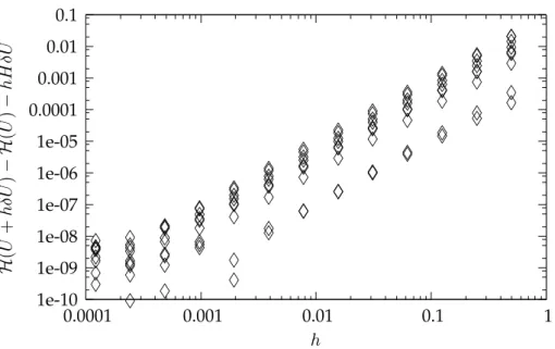
Figure 1: Validation of the tangent construction. For a given h, evaluation of H(U +hδU )−H(U )− hHδU for 18 float trajectories, after 6 days.
2.4 Tangent and adjoint observation operators The tangent model of H writes at time k:
δXk= δXk−2+ 2∆t δUk−1, δXk= eFαk(δαk), δak= eAαk(δαk), δUk= 2 X i,j=1 aijδUk(Qij) + 2 X i,j=1 δak,ijUk(Qij), (6)
where eAis the tangent model of operator A, and Uk, δUkare the direct and tangent model of the
velocity field. The adjoint model is easily deduced from the tangent one. Figure1illustrates the linear tangent hypothesis in the GYRE configuration, for 18 floats, after 6 days: for an increment of the velocity model hδU , with varying h, one observes a behaviour of the quantity H(U +hδU )− H(U ) − hHδU in O(h2).
Listing 1: Adjoint test output for the Lagrangian Observation Operator - with ORCA2 - for 18 float trajectories - after 6 days.
Routine (L) ( L * dx )ˆT W dy dxˆT LˆT W dy Rel. Mach. Status
Err. Eps.
--- --- --- ---- ---
---dia_obs_adj T1 No T profile observations
dia_obs_adj T2 No S profile observations
dia_obs_adj T3 No SLA observations
dia_obs_adj T4 No SST observations
dia_obs_adj T5 .680160300861511E+02 .680160300861511E+02 .4E-15 .2E-15 warning
For a perturbation δX on the state variable, it consists in the comparision of the two scalar products: The classical test to validate and adjoint HT of a linear operator H is:
< HδX, Y >and < δX, HTY > .
In NEMOVAR, the test is made with a particular choice of Y : Y = HδX, and we have chosen to implement the same test for the adjoint model related to (6). Listing1shows the validation of our adjoint model in the ORCA configuration. For line T1 – T5, the component of the state variable linked to the observed variable is perturbated; second and third columns show the scalar product values, forth and fifth columns are the relative error between these two scalar products, and the expected machine error. Line T5 stands for the Lagrangian Observation Operator only, for which an analyticial velocity model is given, depending on space and time coordinates. In Line T6, all the components of the state variable are perturbated, and the sum of all the scalar products with respect to each observation operator is done. In this case, the velocity field is constant, implying a different result from the Lagrangian tangent and adjoint model viewpoint: the two scalar products are different from line T5.
One task was then to develop the tangent and adjoint procedures associated to this interpola-tion method, as well as the tests of these procedures on the main test configurainterpola-tions GYRE and ORCA2 . Their implementation in NEMOVAR has required a specific application, in order to be consistant with the conventions and data structures already presents in NEMOVAR.
One aim of the development of these routines was to make the assimilation of Lagrangian Data possible for users of NEMOVAR. This has then required an implementation in the code with the respect to the philosophy of the other observation operators, in term of fortran data structures as well as interface with the user. A reference manual has also been writtenChauvin(2010).
2.5 An adapted implementation of grid search for Lagrangian data.
The specific nature of Lagrangian particles is that they move according to the model velocity field. At each time step of the algorithm, one need to find the cell Cjthat contains the particle. The actual
obs grid searchalgorithm consists in looking among all the grid cell, and is aimed to initialize the observation positions in the geographical grid. Such an algorithm is not appropriate when the positions have to be evaluated at each time step.
A way to tackle this issue is to make a quick search for particle at time tnknowing its grid cell at
time tn−1: indeed, the time step is small enough to guarantee that the particule either stays in the
same cell, or goes to a neighbor cell. In this viewpoint, the Lagrangian nature of particles allows to construct an efficient grid search.
3
Reference Manual of the Lagrangian Observation Operator in NEMOVAR
The code structure for Lagrangian Observation Operator follows the philosophy of the other ob-servation operators. Specific directories have been created in NEMO and NEMOVAR, and the modules contained therein are detailed in the next subsection. Then, a specific attention is given to the Fortran structure type obs_lag defining the Lagrangian observation objet, and to the con-struction of the Lagrangian observation operator (module obs_lag_adv).
3.1 Lagrangian observation operator modules in NEMO The following files are located in NEMO/OPA_SRC/LAG directory:
obs_lag_adv.F90 ! Update the Lagrangian observation data structure at each time step
obs_lag_def.F90 ! Definition of the Lagrangian observation type
obs_lag_read.F90 ! Read the float coordinates
obs_lagrangian.F90! Storage space for Lagrangian observations
obs_lag_write.F90 ! Write observation and model equivalent to a file
File obs_lagrangian is the equivalent of obs_profiles.F90. File obs_lag_def contains also allocation and deallocation routines of obs_lag data type objects.
As for the other observations, the Lagrangian data structure is loaded from the dia_obs_init routine of module diaobs. Three namelist parameters have been added to the namelist namobs:
ln_lag: logical flag that enables Lagrangian observation operator lagfiles: list of observation files
ln_ena_lag: Load the float observations from a feedback file, or a profile file.
For the moment, last flag ln_ena_lag has been implemented but not tested. Some problems are still present during the read of Netcdf files, written in Feedback format or not. The input file format is the following: first line contains the number of floats, and then each line contains the following fields: float number, time step, position (λ, φ, z) of the observation, and position of its model equivalent.
3.2 The Lagrangian data structure
The data structure obs lag defined below contains the general information on the Lagrangian ob-servation: the number of floats (nlag), the number of time steps of the direct model nstp, as well as other parameters such as the structure isin (tells if there is an observation of float j at time tk
for each float and each time step), counters of enabled / disabled floats (nout, kout), depth of each float (mk: constant and read from input file), beginning and end of observation for one float (fields ista and iend).
Object obs_lag contains fields called var: they correspond to the information needed for the zonal and meridional component: mesh grid index (mi and mj), observed position and its coun-terpart (vobs and vmod), as well as additional informations located in table vext (for instance float velocity at each time step...) and rext (for instance component of the matrix R). The coordi-nates of a float at time tkis contained in (var(1)%vmod(kt),var(2)%vmod(kt)).
Listing 2: obs lag derived type
TYPE obs_lag
INTEGER :: &
& nlag, & !: Number of floats
& nstp, & !: Time step of each trajectory
& nstpup,& !: Time step of each trajectory
LOGICAL, POINTER, DIMENSION(:,:) :: &
& isin !: true while the particle stays inside the domain
INTEGER, POINTER, DIMENSION(:):: &
& nout, & !: Number of outgoing float
& kout, & !: Index when outgoing float
& ista, & !: Time index for the first observation time
& iend, & !: Time index for the last observation time
& mk !: k-th grid coordinate for interpolating X data
TYPE(obs_lag_var), POINTER, DIMENSION(:) :: &
& var !: coordinates in real space
REAL(wp), POINTER, DIMENSION(:,:,:) :: & !:
& lmask !: land/ocean mask at T-, U-, V- and F-points
END TYPE obs_lag
Listing 3: obs lag var derived type
TYPE obs_lag_var
INTEGER, POINTER, DIMENSION(:,:):: &
& mi, & !: i-th grid coordinate for interpolating X data
& mj !: j-th grid coordinate for interpolation X data
REAL(KIND=wp), POINTER, DIMENSION(:,:) :: & !: coordinates in real space
& vobs, & & vmod, &
& rext !: extra variable
REAL(KIND=wp), POINTER, DIMENSION(:,:,:) :: &
& vext !: extra variable
END TYPE obs_lag_var
In NEMO, only the float velocities are used and updated during the observation diagnos-tics. They correspond to the component var(i)%vext(:,1,:) of object obs_lag_var. In NEMOVAR, other quantities as to be saved during the computation, namely the tangent vari-ables, the weighted misfit, etc. The definition of these different components is done in module lag_obspointof NEMOASSIM/VAR_SRC/LAGTAM, keeping the code structure of other observa-tion operators.
Listing 4: Lagrangian observation related global variables
INTEGER, PARAMETER :: mlagcoast = 11 ! Distance to coast
!!! mlagvelo must be equal to 1 (used in nemo) !!!
INTEGER, PARAMETER :: mlagvelo = 1 ! Velocity associated to component var
INTEGER, PARAMETER :: mlagvtan = 2 ! Tangent linear particle velocity
INTEGER, PARAMETER :: mlagberr = 3 ! Background error
INTEGER, PARAMETER :: mlagctan = 4 ! Tangent linear coordinate
INTEGER, PARAMETER :: mlagcwdt = 5 ! Weighted misfit
INTEGER, PARAMETER :: mlagvwdt = 6 ! Weighted misfit
!!! mlagdep must be equal to 1 (used in nemo) !!!
INTEGER, PARAMETER :: mlagdep = 1 ! Depth
INTEGER, PARAMETER :: mlagoerr = 2 ! Observation error
3.3 The Lagrangian observation operator
The direct lagrangian model is contained in file obs_lag_adv, which is composed of three rou-tines:
Listing 5: obs lag dev module’s header
MODULE obs_lag_adv
PUBLIC &
& obs_lag_adv_stp, &
!!---!!
!! ** Purpose : Advance Float positions at each time step: compute the
!! model counterpart of float positions
!!
!! ** Method : Update float velocity with the interpolation of U, V
!! at each float position and then
!! Explicit Euler scheme for updating positions.
!!---& obs_lag_intp, & !:
!!---!!
!! ** Purpose : Interpolate the model velocity at each float position
!! located inside the domain
!!
!! ** Method : Compute float velocity by an interpolation of U, V
!! at each float position.
!! Interpolation scheme k2dint = 3 available only
!! (single interpolation scheme that is differentiable
!! w.r.t. velocity model)
!!---& obs_lag_dom_chk !:
!!---!!
!! ** Purpose : Checks that the updated lagrangian positions belongs
!! to the domain
!!
!! ** Method : Loop on the floats positions, and check that they
!! belong to the U grid and the V grid.
!!
!! ** Action : Compute the logical field obs_lag%isin
!! as well as cell indices (mi,mj) in grids U and V.
!!---For a given time step, routine obs_lag_adv_stp computes the new float positions following a leap-frog scheme. In obs_lag_intp, float velocities are updated by mean of an interpolation of the model velocity at float positions. Finally, obs_lag_dom_chk checks and counts the floats that are still inside the domain, and computes the indices of the mesh grid that contains each float.
During the initialization of the Lagrangian data structure (in routine obs_lag_init, of module obs_lag_read), the fields mi and mj are initialized for each time step and each float: this is essential since in NEMOVAR the adjoint model is applied from nitend to nit000 with no direct model computation: the grid coordinates have to be computed once from the model equivalent of the float positions.
3.4 Tangent and adjoint models of the Lagrangian Observation Operator
Tangent and adjoint models for the assimilation of float position are implemented in the directory LAGTAMof NEMOASSIM/VAR_SRC. This directory contains the following modules:
lag_obs_inter_tam.F90 ! TL and AD model counterpart of lagrangian obs., and TL test
lag_obs_oper_tam.F90 ! Tangent and adjoint routines of the Lagrangian obs. operator
lag_obspoint.F90 ! Pointers for variable numbers in obs_lag structure
lag_obsstore.F90 ! Storage space for Lagrangian observations
Module lag_obs_inter_tam contains a set of tangent and adjoint routines associated to the bilinear remapping interpolation scheme presented in section2.3. The other routines of this module are called by the two routines presented. By then they are not mentionned for the sake of simplicity. It corresponds respectively to the third and second lines of System (6).
Listing 6: lag obs inter tam module’s header
MODULE lag_obs_inter_tam
PUBLIC &
& obs_int_h2d_init_tan, & ! TL Hor. interpolation to the observation point
!!---!! ** Purpose : Computes TL weights for horizontal interpolation to the
!! observation point, for lagrangian data.
!!---& obs_int_h2d_tan , & !
!!---!! ** Purpose : Impact of TL weights
!!---& obs_int_h2d_init_adj, &
!!---!! ** Purpose : Propagation of AD weights for lagrangian data.
!!---& lag_obs_int_h2d_adj , & !
!!---!! ** Purpose : Impact of the model on AD weights
!!---& obs_int_h2d_adj_lag , & !
!!---!! ** Purpose : Impact of AD weights on the state variable
!!---Module lag_obs_oper_tam is composed by the tangent and adjoint lagrangian observation operators, and calls the previous routines.
Listing 7: lag obs oper tam module’s header
MODULE lag_obs_oper_tam
PUBLIC obs_lag_opt_tan, &
!!---!! ** Purpose : TL position and velocity for lagrangian data
!!---& obs_lag_opt_adj, & ! Compute the AD model counterpart of lagrangian obs.
!!---!! ** Purpose : Adjoint model for Lagrangian Observation Operator
!!---& obs_lag_opt_tan_tst ! TL test
!!---!! ** Purpose : Test the tangent routine for lagrangian data.
!!---The Lagrangian Observation Operator is the only observation operator that is non linear with respect to the state variable, since the float position depends on the model velocity. The tangent operator is a linear approximation of the direct operator, and is validated in the routine that tests the adjoint model of observation operators dia_obs_adj_tst. In this routine, a fifth part has been added to test the Adjoint model of Lagrangian observation operator. It has to be underlined that here, we have implemented the test for an analytical model velocity, in order to validate the code not only for a single time step, but also for a full float trajectory.
4
Demonstrator for the twin experiments
The information of this part are available on the VODA project websitehttp://voda.gforge. inria.fr.
A
APPENDIX : Subtasks, milestones and deliverables for Task 2.3
Subtask 2.3.1: Identical twin experiments.
Identical twin experiments will be performed in the low-resolution model, in order to validate the assimilation of Lagrangian data. The main work of this subtask will be the correct formulation of the Lagrangian observation operator.
Subtask 2.3.2: Non-identical twin experiments: the representativeness error issue.
Then, the problem of the representativeness error must be addressed. Indeed, in the real ocean, Lagrangian drifting floats are subject to the full range of scales of the fluid motion, while the reso-lution of the ocean model filters the smaller scales. We will generate high-resoreso-lution observations using the high-resolution component of WP4 T4.2. Developments of subtask 2.3.1 will be then used to assimilate these pseudo data into the low-resolution data assimilation system. The prob-lem we are likely to face is the modelling of the Lagrangian trajectories into the low- resolution model. This issue could be addressed by adding new terms in the floats advection equation, e.g., stochastic noise, smaller scale parameterization. Should this approach fail, we would try instead to filter the high-resolution data before assimilation, and propose a satisfying pre-processing of the Lagrangian data. Another point of this subtask is to assess the complementarities between the Lagrangian position data, and two other types of data: temperature and salinity profiles, altimetry. At this point we will be able to optimize the observing system design in the given domain. Subtask 2.3.3: Real data assimilation.
This will be done in the framework of WP4 T4.3, using developments and expertise from the previous subtasks. The issue specifying the measurement error will have to be specifically ad-dressed. For Argo floats, errors come mainly from the wind-induced drift of the float at the sur-face of the ocean. Indeed, the floats are located by GPS, but there are some gaps in time between the arrival of the float at the surface and the moment it is first seen by the satellite. These drifts depend on the surface wind and surface currents, so that they are inhomogeneous in time and in space.
Milestone:
M 2.3 implementation of the observation operator for the general case (subT2.3.2, T0+18). Deliverables:
• D 2.3.1: Documentation of the observation operator. Demonstrator for the twin experiments. (T0+12)
• D 2.3.2: Documentation of the corrected observation operator and/or the adequate pre-processing of the Lagrangian positions. Demonstrator for the twin experiments. (T0+24) • D 2.3.3: Documentation of the modelling of real errors and the pre-processing of real data.
Demonstrator for the real data assimilation experiments. (T0+36) Demonstrators will consist of a web page accessible from the project web site. It will describe the method and show some results.
APPENDIX : Acronyms • NEMO : Nucleus for European Modelling of the Ocean. • NEMOTAM : TAM pour NEMO
• NEMOVAR : Variational Data Assimilation System for NEMO • OPA : Ocean Parall´elis´e. Direct ocean model, component of NEMO. • OPATAM : TAM for OPA 8.x
• OPAVAR : Variational Data Assimilation System for OPA 8.x • ORCA : Global grid for OPA
References
Chauvin, C. (2010), Assimilating lagrangian observations - reference manual, Technical report, VODA.