Carbon Tax Revenue and the Budget Deficit:
A Win-Win-Win Solution?
Sebastian Rausch and John Reilly
Report No. 228
August 2012
The MIT Joint Program on the Science and Policy of Global Change is an organization for research, independent policy analysis, and public education in global environmental change. It seeks to provide leadership in understanding scientific, economic, and ecological aspects of this difficult issue, and combining them into policy assessments that serve the needs of ongoing national and international discussions. To this end, the Program brings together an interdisciplinary group from two established research centers at MIT: the Center for Global Change Science (CGCS) and the Center for Energy and Environmental Policy Research (CEEPR). These two centers bridge many key areas of the needed intellectual work, and additional essential areas are covered by other MIT departments, by collaboration with the Ecosystems Center of the Marine Biology Laboratory (MBL) at Woods Hole, and by short- and long-term visitors to the Program. The Program involves sponsorship and active participation by industry, government, and non-profit organizations.
To inform processes of policy development and implementation, climate change research needs to focus on improving the prediction of those variables that are most relevant to economic, social, and environmental effects. In turn, the greenhouse gas and atmospheric aerosol assumptions underlying climate analysis need to be related to the economic, technological, and political forces that drive emissions, and to the results of international agreements and mitigation. Further, assessments of possible societal and ecosystem impacts, and analysis of mitigation strategies, need to be based on realistic evaluation of the uncertainties of climate science.
This report is one of a series intended to communicate research results and improve public understanding of climate issues, thereby contributing to informed debate about the climate issue, the uncertainties, and the economic and social implications of policy alternatives. Titles in the Report Series to date are listed on the inside back cover.
Ronald G. Prinn and John M. Reilly Program Co-Directors
For more information, please contact the Joint Program Office
Postal Address: Joint Program on the Science and Policy of Global Change 77 Massachusetts Avenue
MIT E19-411
Cambridge MA 02139-4307 (USA)
Location: 400 Main Street, Cambridge
Building E19, Room 411
Massachusetts Institute of Technology
Access: Phone: +1.617. 253.7492
Fax: +1.617.253.9845
E-mail: [email protected]
Web site: http://globalchange.mit.edu/
1
Carbon Tax Revenue and the Budget Deficit: A Win-Win-Win Solution? Sebastian Rausch* and John Reilly*†
Abstract
Bush-era tax cuts are scheduled to expire at the end of 2012, leading to interest in raising revenue through a carbon tax. This revenue could be used to either cut other taxes or to avoid cuts in Federal programs. There is a body of economic research suggesting that such an arrangement could be a win-win-win situation. The first win—Congress could reduce personal or corporate income tax rates, extend the payroll tax cut, maintain spending on social programs, or some combination of these options. The second win—these cuts in income taxes would spur the economy, encouraging more private spending and hence more employment and investment. The third win—carbon dioxide (CO2)
pollution and oil imports would be reduced. This analysis uses the MIT U.S. Regional Energy Policy (USREP) model to evaluate the effect of a carbon tax as part of a Federal budget deal. A baseline scenario where temporary payroll cuts and the Bush tax cuts are allowed to expire is compared to several scenarios that include a carbon tax starting at $20 per ton in 2013 and rising at 4%. We find that, whether revenue is used to cut taxes or to maintain spending for social programs, the economy is better off with the carbon tax than if taxes remain high to maintain Federal revenue. We also find that, in addition to economic benefits, a carbon tax reduces carbon dioxide emissions to 14% below 2006 levels by 2020, and 20% below by 2050. Oil imports remain at about today’s level, and compared to the case with no carbon tax, are 10 million barrels per day less in 2050. The carbon tax would shift the market toward renewables and other low carbon options, and make the purchase of more fuel-efficient vehicles more economically desirable.
Contents
1. INTRODUCTION ...1
2. POLICY SCENARIOS ...3
3. ECONOMY-WIDE ECONOMIC IMPACTS ...6
4. EFFECTS ON CARBON DIOXIDE EMISSIONS ...9
5. CARBON TAX REVENUE AND TAX RATES ...9
5. ECONOMIC EFFECTS BY INCOME LEVEL ... 12
6. OIL IMPORTS ... 15
7. SUMMARY ... 16
8. REFERENCES ... 17
1. INTRODUCTION
The U.S. faces a large Federal deficit and all parties recognize the need to eventually bring it under control. The recession greatly exacerbated the deficit situation by reducing tax receipts because economic activity fell and because temporary tax cuts (reduction in the payroll tax, Bush tax cut extension) were enacted. On the expenditure side, stimulatory deficit spending (e.g., the American Recovery and Reinvestment Act), automatic increases in spending (e.g., higher unemployment leading to more spending on unemployment benefits), and extension of benefits of these programs (e.g., lengthening the period of eligibility for unemployment) also contributed to the deficit.
* Joint Program on the Science and Policy of Global Change, Massachusetts Institute of Technology, Cambridge,
MA, USA.
2
These are all temporary conditions and Congressional Budget Office (CBO, 2011b) analysis indicates that with current law and return to more normal economic conditions the deficit would fall. But even with the removal of these temporary influences the debt-to-GDP ratio would rise to 77% by 2021, far above the roughly 35 to 40% that was maintained for the most of post-World War II period. CBO also notes that “current law” includes many provisions that may be changed or extended, but unfortunately most of the changes being discussed would have further negative consequences for the deficit. Examples include further extension of at least some part of the Bush tax cuts, indexing of the Alternative Minimum Tax (AMT), originally intended for only the very wealthy but now affecting many more people, or failure to follow through with Medicare reductions for physician payments.
The recognition of the long-term deficit problem was largely responsible for the agreement, as part of last summer’s effort to raise the debt ceiling, that if deficit reduction could not be
reached, automatic cuts to defense and social programs would take effect. That agreement was intended to create the incentive for both political parties to negotiate in good faith, with
Republicans particularly motivated to stave off cuts to defense and Democrats wanting to avoid cuts to social programs.
While raising taxes is never popular, a carbon tax is potentially a win-win-win solution. First, carbon tax revenue can allow revenue-neutral relief on personal income taxes, corporate income tax, or payroll taxes, or could be used to avoid or limit cuts to social programs (Medicare, Medicaid, Social Security, Food Assistance) or Defense spending. Among the revenue raising options evaluated by the CBO was a carbon tax that would start at $20 in 2012 and rise at a nominal rate of 5.8% per year, approximately 4% in real terms given the underlying inflation rate they projected. By their estimate it would raise on the order of $1.25 trillion over a 10-year period. Second, economic analysis has demonstrated the potential for a tax interaction effect whereby recycling of revenue from a carbon tax to offset other taxes could reduce the cost of a carbon policy or even under some circumstances boost economic welfare (Bovenberg and Goulder, 1996). The Bush tax cuts and other temporary tax relief measures are due to expire at the end of 2012. A carbon tax could allow their further extension. And, third, a carbon tax would lower fossil fuel use, reducing carbon dioxide emissions; and lowering oil imports.
The effects of this last “win” would spread across the energy sector. With the new
requirements for improved vehicle efficiency the higher tax-inclusive gasoline price would make fuel efficient vehicles more attractive to consumers and thus make it easier for automobile producers to sell a fleet that meets the efficiency requirements. With a more efficient fleet, even though gasoline prices would rise, the actual fuel cost of driving could fall. A carbon tax would also create support for renewable fuels and electricity. Provisions to stimulate these alternative sources have often involved tax expenditures—investment in or production of renewable energy gives companies a tax credit, thereby reducing tax revenue and aggravating the deficit. The investment and production tax credits for renewable electricity are due to expire, and with the looming deficit it would be more difficult to justify their continuation. A carbon tax would
3
continue to provide encouragement for these technologies by making dirtier technologies more expensive, and raise revenue rather than spend it.
To investigate the potential tradeoffs among different strategies for reducing the deficit we use the MIT U.S. Regional Energy Policy (USREP) model. USREP has been widely used to investigate energy and climate policy, including interactions with tax policy, and effects on economic growth, efficiency, and distribution (Rausch et al., 2010, 2011a,b; Caron et al., 2012). The version we apply here is that in Rausch et al. (2010). We find that any of several different options for using the carbon tax revenue would generate a win-win-win solution. Given that all other options for dealing with the Federal deficit require difficult tradeoffs, it would seem hard to pass up one that offers so many advantages.
2. POLICY SCENARIOS
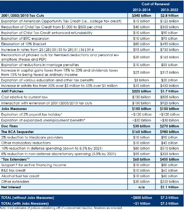
As our reference we use USREP to create a baseline scenario where the temporary payroll cuts and Bush tax cuts expire as scheduled under current law. We use estimates from the Committee for a Responsible Budget (2012) on revenue effects of these tax changes in 2013 to adjust personal income tax rates upward. 1 We include those items listed as tax cuts, AMT patches, and jobs measures shown in Table 1.
We then create several scenarios using USREP that include a carbon tax starting in 2013 at $20 per ton and rising at 4% in real terms to match the CBO assumption. CBO results are in nominal dollars, with an assumed inflation rate, and so their rate of carbon price increase is higher. USREP solves in real terms—we adjust the key revenue projections to nominal dollars using CBO assumed inflation rates to make a ready comparison. All of our scenarios enforce revenue neutrality and so the carbon tax revenue allows us to cut other taxes or to avoid
reductions to social programs. We consider two options (1) All of the carbon tax revenue, after assuring revenue neutrality, is used for tax relief or social programs (2) One half of the revenue is used to fund an investment tax credit, and any remainder, after assuring revenue neutrality, is used for tax relief.2
1
We adjusted all marginal tax rates upward proportionally.
2 There has been interest in using revenue to fund R&D. Our modeling system does not allow us to separately
identify general investment and R&D or to easily target specific types of R&D and so we implement this as a general investment tax credit.
4
Table 1. The fiscal impact of policies that expire or activate in or after 2012.
Source: Committee for a Responsible Budget (2012).
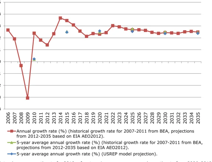
The model base year is 2006. We benchmark economic growth through the present based on historical data, and to the Energy Information Administration (EIA) 2012 Annual Energy
Outlook median forecast for the future, extending that growth rate through 2050. Figure 1 shows our projected 5-year growth rates with the EIA annual forecasts. For near term and historical years, where there is considerable inter-annual variability, our 5-year growth rates are an average. Thus, for example, our growth rate from 2006 to 2010 is near zero, and average of
5
positive growth rates in 2007 and 2010 with the recession years of 2008 and 2009. We also impose existing U.S. Corporate Average Fuel Economy (CAFE) standards, and adjust energy efficiency improvements in the model. With these changes, our emissions match history and are slightly higher in the reference case than the EIA projection. We show this comparison in Figure
4, when we discuss the impact of the carbon tax on CO2 emissions.
Note: Average growth rate for 2010 refers to a 4-year average annual growth rate from 2006–2010.
Figure 1. Baseline GDP. GDP growth rate for reference case: Model versus historic BEA and
EIA/AEO2012 projections.
For each of these two broad options we have four scenarios where we use the carbon tax revenue to cut either personal income tax rates, corporate income tax rates, payroll taxes or to offset reductions in transfer payments. 3 Transfer payments combine Social Security, Medicare, Medicaid, and other such programs. We do not distinguish among these individual programs. However, these payments end up in households with low earned income, and so the general distributional effect of this use of revenue is reflected in our results.
3
Defense cuts or using funds to avoid defense cuts are also likely to be an important part of the political discussion but we do not have a good way to value different levels of defense expenditure. Simply increasing government expenditure on defense would generally show a loss to the economy because we have no way of valuing the increased security those expenditures would bring.
-4 -3 -2 -1 0 1 2 3 4 5 2 0 0 6 2 0 0 7 2 0 0 8 2 0 0 9 2 0 1 0 2 0 1 1 2 0 1 2 2 0 1 3 2 0 1 4 2 0 1 5 2 0 1 6 2 0 1 7 2 0 1 8 2 0 1 9 2 0 2 0 2 0 2 1 2 0 2 2 2 0 2 3 2 0 2 4 2 0 2 5 2 0 2 6 2 0 2 7 2 0 2 8 2 0 2 9 2 0 3 0 2 0 3 1 2 0 3 2 2 0 3 3 2 0 3 4 2 0 3 5
Annual growth rate (%) (historical growth rate for 2007-2011 from BEA, projections from 2012-2035 based on EIA AEO2012).
5-year average annual growth rate (%) (historical growth rate for 2007-2011 from BEA, projections from 2012-2035 based on EIA AEO2012).
6
All of these scenarios, summarized in Table 2, are carefully designed to ensure that Federal tax revenues are unchanged across scenarios even though the tax rates and levels of economic activity or government payments for social programs are changing. We are interested in economic cost, environmental benefit, and oil import effects of these options. We are also interested in distributional effects: how does each scenario affect, on average, households at different income levels?
Table 2. Scenarios. Name Scenario
Ref Current law with Bush tax cuts and payroll tax cuts expiringa
CTPersInc Carbon taxb revenue used to reduce the personal income tax rates
CTCorp Carbon tax revenue used to reduce corporate tax rates
CTPayroll Carbon tax revenue used to reduce payroll taxes
CT½PersInc As in CTPersInc but ½ of revenue diverted to investment
CT½Corp As in CTCorp but ½ of revenue diverted to investment
CT½Payroll As in CTPayroll but ½ of revenue diverted to investment CTTransfers Carbon tax revenue is used to increase transfer payments CT½Transfers As in CTTransfers but ½ of the revenue is diverted to investment
a Based on estimates of revenue impacts of these taxes made by the Committee for a Responsible
Budget (2012). See Table 1.
b Revenue endogenously determined based on a carbon tax of $20 per ton rising at 4% real. To
match CBO assumptions the carbon tax is at $20 in 2012 dollars. All values in USREP are in constant 2006 dollars, and so we use the CPI estimates and projections from CBO (2011a) to adjust $20 in 2012 to 2006 dollars. For purposes of comparing revenue we inflate revenue at 1.8% to account for inflation assumptions in the CBO analysis. Data on inflation are provided in back-up tables to the main document.
3. ECONOMY-WIDE ECONOMIC IMPACTS
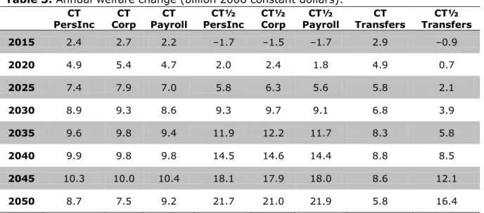
Table 3 and Figure 2 report the annual welfare change in billions of 2006 constant dollars
and as a percentage of total market consumption, respectively.4 For budget purposes and
comparison to the CBO a 10-year horizon is relevant. USREP solves at 5-year time steps and so the first solution period with the carbon tax is 2015. The results are striking in a few ways. First, when we use all of the revenue for tax relief or social programs, we see a net welfare benefit that over time rises to about 0.02%. Second, the scenarios where half of the income is used for an investment tax credit show a much different time path. Here we see initially a net welfare cost of 0.02–0.04% but this turns into a net benefit by 2025 and that benefit continues to increase over time, with the welfare benefit surpassing that in the other cases after 2030 or 2035. Third, we see the initially surprising result that in both the full and half revenue cases, in early years the use of funds for social programs shows the highest welfare result among the different uses for the carbon tax revenue. We turn to a brief discussion of these results.
4 Welfare is the change in aggregate market consumption plus change in leisure. Market consumption is the major
component of GDP (i.e. GDP = Consumption +Investment + Government + Exports–Imports. Leisure time changes because of changes in employment. We report the change as a percent of total aggregate consumption rather than consumption plus leisure because the amount of time accounted as “leisure” or non-work time is somewhat artificial, and set to represent the potential labor force, with a calibrated labor supply elasticity.
7
Table 3. Annual welfare change (billion 2006 constant dollars).
CT
PersInc Corp CT Payroll CT PersInc CT½ CT½ Corp Payroll CT½ Transfers CT Transfers CT½ 2015 2.4 2.7 2.2 –1.7 –1.5 –1.7 2.9 –0.9 2020 4.9 5.4 4.7 2.0 2.4 1.8 4.9 0.7 2025 7.4 7.9 7.0 5.8 6.3 5.6 5.8 2.1 2030 8.9 9.3 8.6 9.3 9.7 9.1 6.8 3.9 2035 9.6 9.8 9.4 11.9 12.2 11.7 8.3 5.8 2040 9.9 9.8 9.8 14.5 14.6 14.4 8.8 8.5 2045 10.3 10.0 10.4 18.1 17.9 18.0 8.6 12.1 2050 8.7 7.5 9.2 21.7 21.0 21.9 5.8 16.4
First, why are there positive net benefits in the full transfer (CT Transfer) case? Here we are seeing the tax interaction effect we noted in the introduction, originally described by Bovenberg and Goulder (1996). Use of the carbon tax revenue to cut distortionary taxes used to fund these transfers reduces the drag they place on the economy enough to more than offset the cost of the carbon tax. Thus we see the economic benefit of raising revenue through a carbon tax as opposed to increases in personal income, corporate income, or payroll taxes. We show in Table 4 the fraction of carbon tax revenue we estimate is needed to maintain revenue neutrality and is thus unavailable for other uses for the CT Transfers case. For tax scoring purposes the Joint
Commission on Taxation (JCT) can require some portion of revenue raised through indirect taxes to be retained to offset general tax losses. In most cases the requirement is that 25% of indirect tax revenue must be retained for revenue neutrality purposes (CBO, 2009). We see a varying fraction over time, averaging slight higher than the standard JCT requirement.
Table 4. Fraction of carbon revenue that is withheld to offset revenue losses from
conventional taxes. Year % 2015 30.8 2020 32.2 2025 34.0 2030 24.4 2035 21.5 2040 24.9 2045 27.3 2050 35.8
8
Second, why do the cases where half of the tax revenue is diverted to an investment tax credit show such a different pattern over time? As noted above, annual welfare is defined as
consumption (and leisure). Diverting revenue to investment reduces the amount available for current consumption, and thus lowers welfare. If used for tax cuts, the higher disposable income would lead to more consumption and investment, and the higher consumption is a contribution to current welfare. But higher investment in the investment tax credit cases leads to a higher capital stock and that makes it possible to produce more goods in succeeding years. The economy grows a bit faster, and so with this growth eventually there is more to consume and welfare then
exceeds the cases without the investment tax credit.
Third, why is welfare higher when revenue is used for social programs? This occurs because it is a transfer of income from relatively higher income households to relatively lower income households. Higher income households save a larger percentage of their income and so in these transfer cases there is more consumption and welfare is thus higher. Eventually, the reduced savings and investment reduces capital stock and the amount of goods that the economy can produce. Thus, while welfare is higher in early years when carbon tax revenue is devoted to social programs it falls below the other cases in later years.
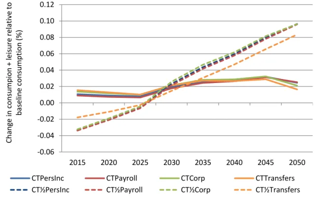
Figure 2. Welfare impacts.
While deficit considerations focus on a 10-year horizon, we have extended the analysis to 2050, with the carbon price continuing to rise at real rate of 4%, because it helps explain the differences above. Without looking over a longer horizon the results would seem to be very peculiar—why doesn’t an investment tax credit look more positive? How can using revenue for
-0.06 -0.04 -0.02 0.00 0.02 0.04 0.06 0.08 0.10 0.12 2015 2020 2025 2030 2035 2040 2045 2050 Ch an ge in c o n sumpio n + leisu re relativ e to b aselin e co n sumptio n (% )
CTPersInc CTPayroll CTCorp CTTransfers
9 2,000 3,000 4,000 5,000 6,000 7,000 8,000 2006 2010 2015 2020 2025 2030 2035 2040 2045 M illi o n m e tric to n o f carbo n dio xide
REF CTPersInc CTPayroll
CTCorp CTTransfers CT½PersInc
CT½Payroll CT½Corp CT½Transfers
EIA (AEO 2012)
social programs lead to higher welfare than other cases that cut taxes and spur the economy? With the extended horizon we see that these scenarios play out as we expect. In the long run an investment tax credit is good for the economy but in the near term more income in the hands of those who are more likely to spend it spurs consumption. A final observation is that the different ways of cutting taxes—personal income, corporate, or payroll—lead to very similar results with some slight differences over time.
4. EFFECTS ON CARBON DIOXIDE EMISSIONS
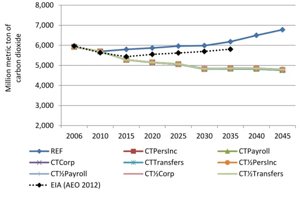
Figure 3 shows carbon dioxide emissions in the reference case without a carbon tax and in
the tax cases. The carbon tax has a significant effect on carbon dioxide emissions. The reference is very similar to recent EIA projections that show little growth in emissions through 2030/2035. After that we begin to see a pick-up in emissions as the economy continues to grow, and some of the effects of new fuel economy standards are fully realized, and then resume growth with economic activity. In the policy cases emissions are 14% below 2006 emissions in 2020, and they continue to drift down over time to about 20% below 2006 in 2050. Those cases with the investment tax credit lead to higher economic activity and somewhat higher emissions in later years but this effect is very small—about a 0.6% difference in 2050.
Figure 3: Carbon dioxide emissions over time. 5. CARBON TAX REVENUE AND TAX RATES
As we noted in the previous section and as shown in Table 4, we estimate that a significant portion of the carbon tax revenue must be retained to cover the general tax revenue penalty
10
because of erosion of the tax base due to the carbon tax. By 2050 this is over one third of the revenue. These results are for the case where we use revenue for social programs.5 Also note that the scenarios allocate fully half of the gross revenue to the investment tax credit, and then the remainder was available for tax relief or social programs. So in the cases with the investment tax credit, by 2050 there is relatively smaller share of revenue left for tax relief or social programs. This is similar to findings in Rausch et al. (2010) using the USREP model. Of course, carbon tax revenue is generally growing over time because the carbon price is increasing at an annual rate of 4% real (5.8% nominal) and emissions are falling at a much slower rate.
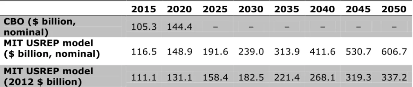
Our estimates of revenue raised by the carbon tax are very similar to those of the CBO (Table
5). As discussed above we adjust our revenue estimates to take account of inflation rates used in
the CBO report. USREP reports values in constant base year dollars (2006). We used data from CBO and their forecasted inflation rate to determine 2012 constant dollars. After 2012 we use an annual 1.6 % inflation rate, approximately the rate assumed in the CBO study (CBO, 2011b). We provide both series. The 2015 CBO revenue estimate is $105.3 billion whereas our comparable nominal dollar estimate is $8.9 billion higher. Given that we are assuming the same carbon price, this obviously reflects somewhat higher emissions in our model—less effect of abatement. By 2020 we are within $3 billion of the CBO estimate. One difference is that we begin the policy in 2013 whereas CBO assumed the policy began in 2012. Given that we are already more than halfway through 2012 as we prepare these results, it would not be plausible to assume that policy begins in 2012. While there is no reason to expect our and CBO estimates to show the same amount of abatement for a given price, they are surprisingly similar in 2020. The somewhat less abatement in 2015 may reflect our capital vintaging, which limits flexibility to abate in the short run.
Table 5. Carbon revenue.
2015 2020 2025 2030 2035 2040 2045 2050 CBO ($ billion,
nominal) 105.3 144.4 – – – – – –
MIT USREP model
($ billion, nominal) 116.5 148.9 191.6 239.0 313.9 411.6 530.7 606.7 MIT USREP model
(2012 $ billion) 111.1 131.1 158.4 182.5 221.4 268.1 319.3 337.2
Source: Congressional Budget Office (2012) “Reducing the deficit: spending and revenue options”, page 205. Inflation assumptions are based on the Consumer Price Index underlying the
projections in Congressional Budget Office (2012). For periods after 2012, we assume an annual inflation rate of 1.6%.
11
As noted, the CBO assumed the policy began in 2012 and estimated a 10-year (2012–2022) revenue of just under $1.25 trillion, a simple sum of nominal dollar revenue in each year. While we only solve every 5 years, if we linearly interpolate revenue using the 3 solution periods (2015, 2020, 2025) that span a 10-year horizon (2013–2023) we estimate the total carbon tax revenue to be about $1.5 trillion.6 One of the reasons this is higher than CBO is the different analysis period. We add in the revenue for year 2023 (estimated to be about $173 billion through our interpolation) and subtract out revenue for the year 2012 (estimate to be just under $100 billion). So that change alone accounts for about $75 billion. Of course, because we only solve every 5 years, our 10-year revenue calculation is a rough approximation. Also, we have not benchmarked out emissions forecast to that of CBO and so their estimates of emissions may differ from ours, either because of a different reference forecast or a difference in abatement for a given carbon price. However, with all these possible differences it is remarkable how close we are in terms of revenue generated.
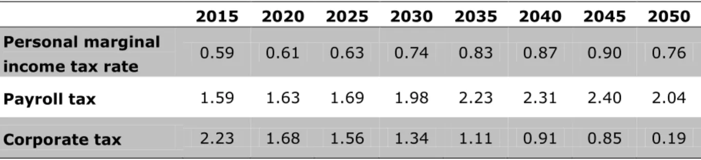
We implement the tax cuts as equal percentage point cuts in the marginal rates for each tax bracket. These tax cuts are endogenously calculated in our model to yield the revenue cost equal to the available carbon tax revenue. The percentage point cuts are given in Table 5 for cases where all the revenue is used for tax relief and in Table 6 for cases where half of the revenue goes to an investment tax credit. In 2015, the available revenue supports an approximate 0.59 percentage cut in marginal personal income tax rates, a 1.59 percentage point cut in the payroll tax, and a 2.23 percentage point cut in the corporate tax rate when 100% of the revenue is available for recycling. These percentage point cuts change over time reflecting changes in the tax base for each category and the revenue available. For the cases where half of the revenue is used for the investment tax credit, the percentage point tax cuts are smaller because less revenue is available. There are also varying effects on economic activity and therefore the tax base and the revenue needed for revenue neutrality.
Table 6. Percentage-points decrease in tax rates (assuming that 100% of carbon revenue is
available for tax recycling).
2015 2020 2025 2030 2035 2040 2045 2050 Personal marginal
income tax rate 0.59 0.61 0.63 0.74 0.83 0.87 0.90 0.76 Payroll tax 1.59 1.63 1.69 1.98 2.23 2.31 2.40 2.04
Corporate tax 2.23 1.68 1.56 1.34 1.11 0.91 0.85 0.19
6
Based on the differences in revenue in the 2 years we estimate, the average difference each year for this period is about $15.6 billion. We multiply this by 10 and add it to the CBO 10 year estimate. Since we are starting in 2013 rather than 2012, we also increase our estimate to account for the fact that our 10 year window includes 2023 and leaves out 2012—this is a nearly $100 billion difference.
12
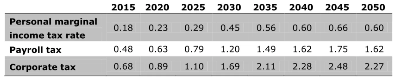
Table 7. Percentage-points decrease in tax rates (assuming that 50% of carbon revenue is
available for tax recycling), “half scenarios”.
2015 2020 2025 2030 2035 2040 2045 2050 Personal marginal
income tax rate 0.18 0.23 0.29 0.45 0.56 0.60 0.66 0.60 Payroll tax 0.48 0.63 0.79 1.20 1.49 1.62 1.75 1.62
Corporate tax 0.68 0.89 1.10 1.69 2.11 2.28 2.48 2.27
5. ECONOMIC EFFECTS BY INCOME LEVEL
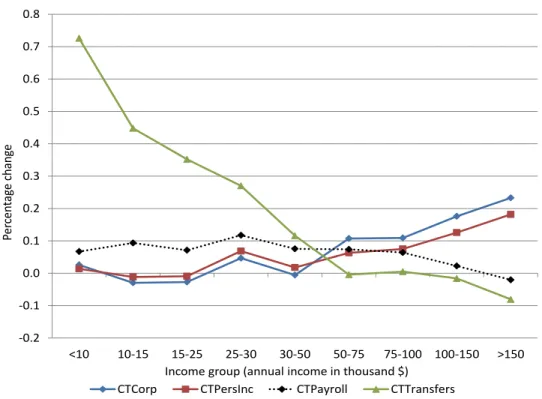
The different uses of revenue have different implications for income groups, shown for 2015 in Figures 4 and 5 and as net present value over the 2015–2050 period in Figures 6 and 7. Not surprisingly, when revenue is devoted to social programs the results are most beneficial to lower income households than in either the case where all net revenue is used for tax relief or social programs (Figure 4) or half is used for the investment tax credit (Figure 5). Households with earned income levels below $100,000 either benefit or are virtually unaffected when all revenue is used to avoid cuts to social programs. This cutoff point drops to the $25,000 to $30,000 earned income level when only half of the revenue is used in this way. The payroll tax cut has the most neutral effect across households of different incomes but is slightly progressive for the highest income households. This general result is expected given the income limitation on the payroll tax—the rate cut is less beneficial for households whose incomes exceed the limit. The income and corporate tax cases are slightly regressive in the case where all revenue is used for tax relief.
Again, this result is not surprising. Higher income households pay more taxes and hence tax cuts benefit them more. The presumed regressivity of energy taxation obtained from partial equilibrium assessments generally does not hold when distributional effects are estimated endogenously as shown in Rausch et al. (2010). This result stems from the fact that low-income households derive more of their income from social programs (e.g., Social Security) that are indexed by price level. This tends to insulate them from effects on income, whereas taxpayers who rely on earned income from labor or capital returns are affected by changes wages and returns to capital. Although as Rausch et al. (2011a) show, the range of effects within any income strata greatly exceeds the difference among income groups. Obviously, some low-income households benefit from transfers, while some do not, and expenditures on energy and other factors vary greatly among households even with the same earned income.
With the investment tax credit using half of the carbon tax revenue welfare levels are lower for all income groups in 2015, and results are generally more progressive (Figure 5). As we saw in Table 3 and Figure 2 the overall welfare levels are lower in this case and so it is not surprising that levels are lower for all households. The relative greater progressivity of the results stem from the fact that tax relief disproportionately benefits those who pay more taxes, generally higher income households. Thus, when less carbon revenue is available for tax relief, higher income households disproportionately lose the tax relief benefit, leading to the more progressive effect.
13 -0.4 -0.3 -0.2 -0.1 0.0 0.1 0.2 0.3 0.4 <10 10-15 15-25 25-30 30-50 50-75 75-100 100-150 >150 Per cen tag e ch an ge
Income group (annual income in thousand $)
CT½Corp CT½PersInc CT½Payroll CT½Transfers
Figure 4: Welfare effects by income group in 2015, all revenue used for tax relief or social
programs. Income levels are defined by earned income only, excluding transfers, and are denominated in constant 2006 dollars.
Figure 5. Welfare effects by income group in 2015, half of the revenue used for investment
tax credit. Income levels are defined by earned income only, excluding transfers, and are denominated in constant 2006 dollars.
-0.2 -0.1 0.0 0.1 0.2 0.3 0.4 0.5 0.6 0.7 0.8 <10 10-15 15-25 25-30 30-50 50-75 75-100 100-150 >150 Per cen tag e ch an ge
Income group (annual income in thousand $) CTCorp CTPersInc CTPayroll CTTransfers
14
Of perhaps more interest are the net present value effects over the 2015–2050 horizon. For this calculation we discount future benefits or costs at a 4% discount rate, and also discount future incomes by the same amount. This creates a discounted average effect over the period. The basic pattern in the cases where all revenue is used for tax relief or social programs is almost identical to the 2015 results. The overall gain to the economy grows over time, and so in general gains are higher for all income groups when summing over the whole period. The slight
exception is over the long term the corporate and personal income tax cases become a bit more regressive so that lower income households are slightly disadvantaged while higher income households benefit more. Again, the payroll tax cut is the most distributionally neutral.
In contrast, the net present value results where half of the revenue is used for an investment tax credit are quite different than the 2015 results. First the net present value results are generally beneficial. This is not surprising as we saw that the investment tax credit cases generate some welfare costs in the near term until the benefits of higher investment are realized in later years. In addition, the distributional pattern is quite different for the net present value results. They look much more similar to the cases without the investment tax credit. Rather than being mostly progressive, they are neutral for the payroll tax cut, and slightly regressive for the personal and corporate income tax cases. This result probably should not be surprising. Those with higher wages and capital returns will benefit more from the investment tax credit because it generally stimulates the economy and their earnings.
Figure 6. Net present value welfare effects by income group, all revenue used for tax relief
or social programs. Income levels are defined by earned income only, excluding transfers, and are denominated in constant 2006 dollars.
-0.2 0.0 0.2 0.4 0.6 0.8 1.0 1.2 <10 10-15 15-25 25-30 30-50 50-75 75-100 100-150 >150 Per cen tag e ch an ge
Income group (annual income in thousand $)
15
Figure 7. Net present value welfare effects by income group, half of the revenue used for
investment tax credit. Income levels are defined by earned income only, excluding transfers, and are denominated in constant 2006 dollars.
6. OIL IMPORTS
Without the climate policy USREP projects a slight increase in imports through 2030, and then a more rapid increase through 2050 (Figure 6). With the carbon tax nearly all of the increase in oil imports is avoided, with imports remaining nearly flat through 2050.
Figure 8. Oil production minus consumption, oil exports—negative number indicates
imports (1970–2006 based on EIA AEO2012, 2007–2050 model projection). -25 -20 -15 -10 -5 0 1970 1975 1980 1985 1990 1995 2000 2005 2010 2015 2020 2025 2030 2035 2040 2045 2050 Do mes ti c p ro d u cti on an d co n sum p ti on (mi lli on b ar re ls p er d ay)
Net imports (baseline)
0.0 0.1 0.2 0.3 0.4 0.5 0.6 0.7 0.8 0.9 <10 10-15 15-25 25-30 30-50 50-75 75-100 100-150 >150 Per cen tag e ch an ge
Income group (annual income in thousand $)
16
7. SUMMARY
The U.S. faces the challenge of bringing its Federal budget deficit under control. There is general recognition that to do so will likely require both difficult budget cuts and enhancements to revenue. One option for revenue enhancement suggested in an earlier Congressional Budget Office (CBO) analysis is the introduction of a carbon tax starting at $20 per ton and rising gradually over time. The CBO estimated that such a carbon tax could raise about $1.25 trillion over the 2012–2022 period. We simulated a similar carbon tax starting in 2013, given that a start in 2012 is no longer realistic. We find a similar, if somewhat higher 10-year revenue gain of about $1.5 trillion. We have slightly higher revenue at the start of the period because we find a little less abatement, and thus higher emissions. Because the period is extended we also gain from adding in revenue from the year 2023, when the carbon price and revenue is considerably higher than it would have been in 2012.
We use a reference case where the Bush tax cuts and the temporary payroll tax cut expire, as under current law. We then evaluate the carbon tax cases where the revenue from that tax allows us to avoid some of the general tax increases or to fund social programs. We consider cases where the revenue is used to avoid increasing the personal income, corporate income, and the payroll taxes. We consider a similar set of cases where the first half of the revenue is used for an investment tax credit and the remainder is used for tax cuts or social programs.
In cases without the investment tax credit, we find that this combination of a carbon tax with general tax cuts improves overall economic performance. As a result we get other benefits of the carbon tax, reduced emissions and lower oil imports, at no cost. This surprisingly positive result comes through the tax interaction effect that has been widely studied. By avoiding increases in general income taxes we avoid their drag on the economy, and the avoided drag is actually greater than the direct cost of the carbon tax. The economy thus benefits. In the cases where we apply one half of the carbon tax revenue toward an investment tax credit we see lower welfare in early years (through 2025) but then the added investment begins to offset the carbon tax cost, leading to positive effects on economic welfare. The investment tax credit leads to continued improvement in economic performance and by 2030 or 2035 welfare in these cases begins to exceed cases without the investment tax credit, and their benefit continues to grow. We also consider devoting the revenue to social programs, and somewhat surprisingly this also led to near-term gains in welfare because it effectively transferred income from wealthier households who spend less of their income. But this case is somewhat less beneficial to the economy as a whole in the long term because of less savings and investment.
We also investigate the implications for households with different income levels. Here the effects are as one might expect. Using funds for social programs benefits low income
households. Personal income and corporate income tax cuts are most favorable for wealthier households, and the payroll tax cut is fairly neutral for most households, but slightly progressive at higher income levels. When half of the revenue is used for the investment tax credit we see a more progressive effect in the short term because taxes are cut less, and wealthier households pay more in taxes, and there is less progressiveness over the full horizon of our study because
17
wealthier households ultimately benefit from the greater investment returns.
We should mention some caveats to these results. The model approach we use assumes full-employment, and at this point the economy remains in a situation of excess unemployment. While further study would be required, the current economic situation may further favor tax cuts as opposed to an investment tax credit, and especially adjustments that put more money in the hands of lower income households. The economy currently suffers from a lack of demand, and lower income households are more likely to spend than save. While saving and investment are ultimately good for the economy, in the current situation it is lack of consumption growth that appears to be holding back investment rather than a lack of funds to invest. Second, we impose absolute revenue neutrality and in our model this requires a generally larger share of revenue retained for this purpose than is required for budget scoring purposes. In general, the Joint Commission for Taxation (JCT) requires a 25% “haircut” on indirect tax revenue. Our estimate of the required haircut varies but on average is closer to 30%. Moreover, as described in CBO (2009) there are some situations where no haircut would be required. In particular, they argue that a cap and trade policy that gave away allowances to taxpaying entities would not require a haircut. In the proposals we examine, the revenue is returned to taxpaying entities via tax cuts and so this may be ruled as requiring no haircut. If so, the revenue available for tax cuts may be greater than we estimate, and thus we might see more benefit.
The country faces difficult tradeoffs in getting the Federal budget deficit under control. In our analysis of a carbon tax, we find a win-win-win situation that requires no tradeoff at all. Carbon tax revenue allows (1) cuts in other taxes, (2) benefits the economy, and (3) reduces CO2
emissions and oil imports. The tradeoffs are mainly whether we want to choose a set of measures that produce higher consumption in the near term, or a path that sacrifices some current
consumption for an investment tax credit that leads to greater benefit in later years. Given current economic conditions, changes that have more immediate benefit may be preferable, but we can hope for a compromise that yields a result that is also beneficial for the country in the longer term.
Acknowledgements
USREP was developed as a special U.S. model project within the Joint Program. We are especially grateful to funding from sponsors of this special project. We also gratefully acknowledge the support of the Joint Program on the Science and Policy of Global Change, funded grants from DOE, EPA and other federal agencies and a consortium of 40 industrial and foundation sponsors. (For the complete list see http://globalchange.mit.edu/sponsors/all).
8. REFERENCES
Bovenberg, A. L., and L. H. Goulder, 1996: Optimal environmental taxation in the presence of other taxes: general equilibrium analyses. American Economic Review 86: 985–1000. Caron, J., S., Rausch and N. Winchester, 2012: Leakage from Sub-national Climate Initiatives:
The Case of California, MIT JPSPGC Report 220, May, 34 p. (http://globalchange.mit.edu/research/publications/2286).
18
CBO, 2009: The Role of the 25 Percent Revenue Offset in Estimating the Budgetary Effects of Legislation, Economic and Budget Issue Brief, Congressional Budget Office, Washington, DC (January).
CBO, 2011a: The Budget and Economic Outlook: Fiscal Years 2011 to 2021 Congressional Budget Office, Washington, DC (January).
CBO, 2011b: Reducing the Deficit: Spending and Revenue Options, Congressional Budget Office, Washington, DC (March).
Committee for a Responsible Budget, 2012: Between a Mountain of Debt and a Fiscal Cliff. (March).
(http://crfb.org/sites/default/files/Between_a_Mountain_of_Debt_and_a_Fiscal_Cliff_5.pdf ). Rausch, S., G. Metcalf, J. Reilly, and S. Paltsev, 2010: Distributional implications of alternative
U.S. greenhouse gas control measures, The B.E. Journal of Economic Analysis & Policy,
10(2): Symposium.
Rausch, S., G.E. Metcalf and J.M. Reilly, 2011a: Distributional impacts of carbon pricing: A general equilibrium approach with micro-data for households, Energy Economics 33(1): S20–S33.
Rausch, S., G. Metcalf, J.M. Reilly and S. Paltsev, 2011b: Distributional impacts of a U.S. greenhouse gas policy: A general equilibrium analysis of carbon pricing. In: G.E. Metcalf (ed.), U.S. Energy Tax Policy, Cambridge University Press, Cambridge, 52–107.
REPORT SERIES of the MIT Joint Program on the Science and Policy of Global Change
Contact the Joint Program Office to request a copy. The Report Series is distributed at no charge.
FOR THE COMPLETE LIST OF JOINT PROGRAM REPORTS: http://globalchange.mit.edu/pubs/all-reports.php
185. Distributional Implications of Alternative U.S. Greenhouse Gas Control Measures Rausch et al.
June 2010
186. The Future of U.S. Natural Gas Production, Use, and Trade Paltsev et al. June 2010
187. Combining a Renewable Portfolio Standard with a Cap-and-Trade Policy: A General Equilibrium Analysis
Morris et al. July 2010
188. On the Correlation between Forcing and Climate Sensitivity Sokolov August 2010
189. Modeling the Global Water Resource System in an Integrated Assessment Modeling Framework:
IGSM-WRS Strzepek et al. September 2010
190. Climatology and Trends in the Forcing of the Stratospheric Zonal-Mean Flow Monier and Weare
January 2011
191. Climatology and Trends in the Forcing of the Stratospheric Ozone Transport Monier and Weare
January 2011
192. The Impact of Border Carbon Adjustments under Alternative Producer Responses Winchester February
2011
193. What to Expect from Sectoral Trading: A U.S.-China
Example Gavard et al. February 2011
194. General Equilibrium, Electricity Generation Technologies and the Cost of Carbon Abatement Lanz
and Rausch February 2011
195. A Method for Calculating Reference
Evapotranspiration on Daily Time Scales Farmer et al.
February 2011
196. Health Damages from Air Pollution in China
Matus et al. March 2011
197. The Prospects for Coal-to-Liquid Conversion:
A General Equilibrium Analysis Chen et al. May 2011
198. The Impact of Climate Policy on U.S. Aviation
Winchester et al. May 2011
199. Future Yield Growth: What Evidence from Historical
Data Gitiaux et al. May 2011
200. A Strategy for a Global Observing System for Verification of National Greenhouse Gas Emissions
Prinn et al. June 2011
201. Russia’s Natural Gas Export Potential up to 2050
Paltsev July 2011
202. Distributional Impacts of Carbon Pricing: A General
Equilibrium Approach with Micro-Data for Households
Rausch et al. July 2011
203. Global Aerosol Health Impacts: Quantifying
Uncertainties Selin et al. August 201
204. Implementation of a Cloud Radiative Adjustment Method to Change the Climate Sensitivity of CAM3
Sokolov and Monier September 2011
205. Quantifying the Likelihood of Regional Climate Change: A Hybridized Approach Schlosser et al. October
2011
206. Process Modeling of Global Soil Nitrous Oxide Emissions Saikawa et al. October 2011
207. The Influence of Shale Gas on U.S. Energy and Environmental Policy Jacoby et al. November 2011 208. Influence of Air Quality Model Resolution on
Uncertainty Associated with Health Impacts Thompson
and Selin December 2011
209. Characterization of Wind Power Resource in the United States and its Intermittency Gunturu and Schlosser
December 2011
210. Potential Direct and Indirect Effects of Global Cellulosic Biofuel Production on Greenhouse Gas Fluxes from Future Land-use Change Kicklighter et al. March 2012 211. Emissions Pricing to Stabilize Global Climate Bosetti et al.
March 2012
212. Effects of Nitrogen Limitation on Hydrological Processes in CLM4-CN Lee & Felzer March 2012
213. City-Size Distribution as a Function of Socio-economic Conditions: An Eclectic Approach to Down-scaling Global
Population Nam & Reilly March 2012
214. CliCrop: a Crop Water-Stress and Irrigation Demand Model for an Integrated Global Assessment Modeling Approach Fant et al. April 2012
215. The Role of China in Mitigating Climate Change Paltsev
et al. April 2012
216. Applying Engineering and Fleet Detail to Represent Passenger Vehicle Transport in a Computable General Equilibrium Model Karplus et al. April 2012
217. Combining a New Vehicle Fuel Economy Standard with a Cap-and-Trade Policy: Energy and Economic Impact in
the United States Karplus et al. April 2012
218. Permafrost, Lakes, and Climate-Warming Methane Feedback: What is the Worst We Can Expect? Gao et al. May
2012
219. Valuing Climate Impacts in Integrated Assessment Models: The MIT IGSM Reilly et al. May 2012
220. Leakage from Sub-national Climate Initiatives: The Case
of California Caron et al. May 2012
221. Green Growth and the Efficient Use of Natural Resources
Reilly June 2012
222. Modeling Water Withdrawal and Consumption for Electricity Generation in the United States Strzepek et al.
June 2012
223. An Integrated Assessment Framework for Uncertainty Studies in Global and Regional Climate Change: The MIT
IGSM Monier et al. June 2012
224. Cap-and-Trade Climate Policies with Price-Regulated Industries: How Costly are Free Allowances? Lanz and
Rausch July 2012.
225. Distributional and Efficiency Impacts of Clean and Renewable Energy Standards for Electricity Rausch and
Mowers July 2012.
226. The Economic, Energy, and GHG Emissions Impacts of Proposed 2017–2025 Vehicle Fuel Economy Standards in the United States Karplus and Paltsev July 2012
227. Impacts of Land-Use and Biofuels Policy on Climate:
Temperature and Localized Impacts Hallgren et al. August
2012
228. Carbon Tax Revenue and the Budget Deficit: A