Three-dimensional numerical analysis technique for interpreting monitored result of the exterior insulation basement systems (EIBS) experiment

(1)

Publisher’s version / Version de l'éditeur:

Vous avez des questions? Nous pouvons vous aider. Pour communiquer directement avec un auteur, consultez la

première page de la revue dans laquelle son article a été publié afin de trouver ses coordonnées. Si vous n’arrivez pas à les repérer, communiquez avec nous à PublicationsArchive-ArchivesPublications@nrc-cnrc.gc.ca.

Questions? Contact the NRC Publications Archive team at

PublicationsArchive-ArchivesPublications@nrc-cnrc.gc.ca. If you wish to email the authors directly, please see the first page of the publication for their contact information.

https://publications-cnrc.canada.ca/fra/droits

L’accès à ce site Web et l’utilisation de son contenu sont assujettis aux conditions présentées dans le site LISEZ CES CONDITIONS ATTENTIVEMENT AVANT D’UTILISER CE SITE WEB.

Internal Report (National Research Council of Canada. Institute for Research in Construction), 2000-09-14

READ THESE TERMS AND CONDITIONS CAREFULLY BEFORE USING THIS WEBSITE. https://nrc-publications.canada.ca/eng/copyright

NRC Publications Archive Record / Notice des Archives des publications du CNRC : https://nrc-publications.canada.ca/eng/view/object/?id=0270e70e-b26b-4579-bd8f-5a3ecd68e3ec https://publications-cnrc.canada.ca/fra/voir/objet/?id=0270e70e-b26b-4579-bd8f-5a3ecd68e3ec

NRC Publications Archive

Archives des publications du CNRC

For the publisher’s version, please access the DOI link below./ Pour consulter la version de l’éditeur, utilisez le lien DOI ci-dessous.

https://doi.org/10.4224/20386128

Access and use of this website and the material on it are subject to the Terms and Conditions set forth at

Three-dimensional numerical analysis technique for interpreting monitored result of the exterior insulation basement systems (EIBS) experiment

Maref, W.; Swinton, M. C.; Bomberg, M. T.; Kumaran, M. K.; Normandin, N.; Marchand, R. G.

(2)

http://irc.nrc-cnrc.gc.ca

T hre e -Dim e nsiona l N um e ric a l Ana lysis

Te chnique for I nt e r pre t ing M onit ore d

Re sult of t he Ex t e rior I nsulat ion

Ba se m e nt Syst e m (EI BS) Ex pe rim e nt

M a r e f , W . ; S w i n t o n , M . C . ;

B o m b e r g , M . T . ; K u m a r a n , M . K . ;

N o r m a n d i n , N . ; M a r c h a n d , R . G .

I R C - I R - 8 1 4

September 14, 2000

(3)

Three-dimensional Numerical Analysis Technique for

Interpreting Monitored Results of the Exterior Insulation

Basement Systems (EIBS) Experiment

Abstract

1

A consortium research project was initiated to determine the field performance of various thermal insulation products as applied in the exterior insulation basement system (EIBS). Initially a two-dimensional analytical tool was used to derive the thermal transmission characteristics from an array of temperature measurements monitored over a period of two years. Results immediately showed the influence of lateral heat flux between various products that differed in thermal transmission properties. Therefore, development of a three dimensional model became imperative, to resolve the order of magnitude of the lateral heat flux in the experimental set-up, and determine the actual in-situ properties of the insulation specimens.

This report gives the theoretical and numerical approaches adopted to develop a three-dimensional computer model of heat transfer. The implicit Spline Method was selected for the problem solver. The applicability of the model was verified using measured data on temperature distributions at several material interfaces. Then the model was used to estimate the effect of lateral heat flows, and to determine the in-situ thermal properties of the insulation specimens.

The report also records experimental details and presents validation results of the analytical approach.

1

The consortium included Expanded Polystyrene Association of Canada, Canadian Urethane Foam Contractors Association, Owens Corning Inc. and Roxul Inc.

(6)

Nomenclature

ρ Density [kg/m³] C Specific heat [ J/kg.K]

i

K Thermal conductivity in x direction [ W/m.K]

j

K Thermal conductivity in y direction [ W/m.K]

k

K Thermal conductivity in z direction [ W/m.K] Q Heat generation [W/m3]

t Time [s]

Subscripts

i Nodal point value j Nodal point value

T0 Initial temperature[oC]

S1, S2 and S3 Boundary surfaces

t Δ Time step [s] z and y x Δ Δ

Δ , , Step of spatial discretisation in x, y and z direction [m]

k Nodal point value s On boundary surface

(7)

Three-dimensional Numerical Analysis Technique for

Interpreting Monitored Results of the Exterior Insulation

Basement Systems (EIBS) Experiment

Background

Over the recent decades, a large proportion of basements in newly built Canadian houses have become used as a habitable space. This, combined with increased requirements for energy conservation, resulted in the development of many insulated basement systems. While thermal insulation may be placed either on the inside or on the outside of the basement wall, the material choice and the insulation placement may affect overall performance of the basement wall. Some external insulation systems, in addition to controlling heat losses, may also increase durability of the basement wall.

In this context, the Canadian thermal insulation industry, working together with the National Research Council, decided to revisit2 the design and performance of external insulation basement systems (EIBS). Over the two-year period from June 1996 to June 1998, ten expanded polystyrene (EPS), two spray polyurethane foam (SPF), two mineral fibre insulation (MFI) and two glass fibre insulation (GFI) specimens were placed on the exterior of the basement wall in an experimental building located on NRC Campus in Ottawa.

This research project involved a number of material and system issues. Material considerations involved selection of existing and new thermal insulation. These products were placed side-by-side on the basement wall to create virtual test compartments. The system considerations involved two different technical solutions to protect the

2

(8)

grade part of the EIBS. Furthermore, different conditions for surface water drainage were implemented on East and West walls of the NRC experimental basement facility.3 Because of the wide scope of the basement research, this project is reported in four parts:

1. Development of analytical tools to increase confidence in the experimental results and facilitate the analysis of the field data

2. Reporting and analyzing results obtained from the experimental basement 3. Placing the thermal and moisture performance of expanded polystyrene in

below-grade application in context of other research (state-of-the-art review to identity future research needs on the material side)

4. Reporting and analyzing the system effects in context of other research (state-of-the-art review to identity future research needs for development of basement systems)

The first part of the EIBS project is addressed in this report, which presents theoretical and numerical aspects of 3-D computer model developed as a part of integrated approach (modelling and testing). The capabilities of this model to enhance the analysis of experimental results will be demonstrated in the papers (Swinton and al) [3-7] and (Maref and al.) [8].

(9)

1. Experimental Approach

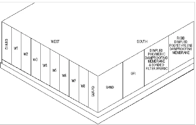
To evaluate the performance of exterior basement insulation, different materials were installed on the exterior surface of concrete basement walls. As shown in Figure 1, eight test specimens were placed side-by-side, on each of two basement walls (east and west) insulating a whole wall with approximately 76-mm thick and 2.4 m high specimens. On the interior of the wall, a 25-mm layer of expanded polystyrene (EPS) board was installed over the entire surface. At 3 vertical locations on each test wall, cut-outs were made and calibrated EPS specimens, with identical thickness, were tightly inserted. These specimens were used for determination of transient heat flux entering the wall (Bomberg and al, 1994) [9].

The monitored temperature difference across the calibrated insulation layer was used to calculate the heat flux profile into the wall on a continuous basis. Detailed analysis of heat transfer through the wall was used to assess the resulting heat flux into each exterior insulation specimen. Using this heat flux and temperature difference across the specimens, the apparent in-situ thermal resistance of the specimens was deduced.

Boundary conditions, including soil temperatures and moisture content were recorded, as well as observations of weather extremes. Four separate soil analyses were performed to characterize the soil environment, including vertical profiles of moisture content. This information was used to qualify differences in observed thermal performance of the specimens.

(10)

Figure 1. Schematic of placement of specimens on the west wall.

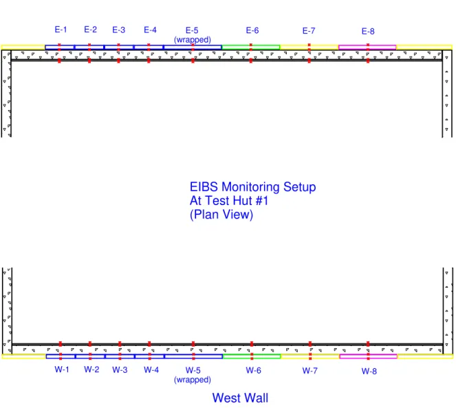
Thermocouples were placed at the boundary surfaces as well as the interfaces of each layer in the wall, in an array consisting of 16 points per test compartment. All sensors placed on the west wall are shown in Figure 2. The east wall sensors were developed in the same way.

(11)

200 mm 18 40 m m 1340 m m Soil thermocouples 1980 mm from wall at top 1370 mm from wall at bot. (locations approx.) Thermocouples in soil 150 m m 740 m m 270 m m West Wall 240 m m

Heat flux transducer (average of 5 emf's)

Heat flux transducer (average of 5 emf's) 4 Thermocouples

4 Thermocouples Heat flux transducer (average of 5 emf's) 4 Thermocouples

4 Thermocouples

Figure 2 Thermocouples and calibrated insulation specimens mounted on the West wall.

The parameters monitored in the EIBS are:

1. Surface temperatures, on both sides of the calibrated specimen, the concrete and the test specimens

2. Heat flux across the calibrated insulation specimens

3. Soil temperatures from 1 to 2 m away from the specimens, and at 5 depths 4. Interior basement air temperature (average of 4 readings)

5. Exterior air temperature (at north face, shielded from sun)

6. Relative humidity (RH) and other parameters of indoor and outdoor environments.

(12)

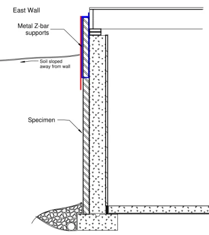
Figure 3. East Wall Configuration East Wall Specimen Metal Z-bar supports Soil sloped away from wall

Figure 3 East-Wall Configuration

Differences between the East and West wall configurations are illustrated in Figures 2 and 3 respectively. The west wall installation had a cantilevered cementitious board that covered the specimens above grade. The grade at the west wall was sloped towards the wall at a 5% grade. The east wall cementitious board was supported by metal Z-bars placed between samples and fastened directly to the concrete. The grade on the east side was sloped at 5% away from the wall.

(13)

A plan view of the arrangement of the specimens is shown in Figure 4. The samples are numbered 1-8 on each wall. Other specimens (guard specimens) consisting of either glass fiber or mineral fiber insulation were also at the extremities of each walls, as shown.

East Wall

West Wall

EIBS Monitoring Setup At Test Hut #1

(Plan View)

W-1 W-2 W-3 W-4 W-5 (wrapped) E-1 E-2 E-3 E-4 E-5

(wrapped)

W-7

W-6 W-8

E-7

E-6 E-8

(14)

The instrumentation package consisted of approximately 145 thermocouples, 2 humidity sensors, 21 calibrated insulation specimens (heat flux transducers), 4 junction boxes, and a data acquisition unit operated by a computer.

1.2 Data acquisition

The collection of data was done with an automated data acquisition and scanning system, and a high precision multi-meter to measure separate thermocouples, serial thermopiles and relative humidity sensors. All thermocouples and power signals were routed through a HP command module (HP E1406) connected to a PC 486/50. Measurements were taken every 2 minutes and averaged by the software package (HP_VEE) for 10-minute intervals for the wall thermocouples (5 readings), and 30-minute intervals for the soil thermocouples (15 readings).

1.3 Duration of the experimental program

The data acquisition system was commissioned in the spring of 1996 and monitoring started on June 5, 1996. The monitoring ended on June 5, 1998, 2 full years of monitoring.

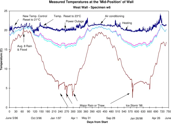
Figure 5 shows measured temperatures of indoor air, calibrated insulation specimens, concrete, and soil surface in the “mid-position” of the wall over a period of two years. The spikes in the interface between soil and the EIBS correspond to thaw periods with a heavy rainfall. Observe that these effects do not appear to affect the temperature on the concrete surface, i.e., behind the external insulation.

(15)

Measured Temperatures at the 'Mid-Position' of Wall 0 5 10 15 20 25 0 30 60 90 120 150 180 210 240 270 300 330 360 390 420 450 480 510 540 570 600 630 660 690 720 750

Days from Start

Temperature (C

)

West Wall - Specimen w6

Oct 3/96

June 5/96 Jan 1/97 Apr 1 New Temp. Control

Reset to 21°C

Aug. 8 Rain & Flood

Temp. Reset to 23°C Power Outage

Major Rain or Thaw

Air conditioning Sep 28 Jan 26/98 Ice Storm '98 Heating Apr 26 June 25 May 31

Figure 5 Temperatures across the W6 specimen measured in the mid-height position.

1.4 Experimental Data

The experimental data set contains a number of time-series records, including • indoor and outdoor air temperatures

(16)

• soil temperatures • soil moisture content

• the temperatures at each material interface in the test wall, at four levels from 50 mm above the slab to 270 mm below grade (see Figure A1 in Appendix A)

• the temperature differences in the reference insulation at three levels measured by lab-assembled heat flux transducers (Figure A2 in Appendix A)

1.4.1 Indoor & Outdoor Air Temperature Profiles

The indoor and outdoor air temperature profiles over the two heating seasons are shown in Figure 6. Data was recorded every half hour. Plotted is every 8th reading, i.e., every 4 hours.

The indoor basement air temperature was held relatively steady at 23°C, with some loss of control experienced in the shoulder seasons. The switch from heating to air-conditioning on the heat pump was manual, resulting in slight overheating of the basement on warm days in spring and fall when the heat pump was set to heating.

The outdoor temperatures show both the diurnal variations and seasonal trends following a rough sine wave. The winter of 1997 featured one very cold night, with temperatures dipping to about -30°C. Neither winters showed a sustained cold snap – each very cold evening was often followed by a thaw (temperatures climbing above 0°C). This unexpected weather pattern may have resulted in low frost penetration, as documented below.

(17)

Indoor and Outdoor Air Temperatures -30 -20 -10 0 10 20 30 40 0 30 60 90 120 150 180 210 240 270 300 330 360 390 420 450 480 510 540 570 600 630 660 690 720 750

Time (days from start)

Tem

p

erat

ure (

°C)

EIBS - Monitoring Results June 5, 1996 - June 8, 1998

June 5/96 Oct 3/96 Jan 1/97 Apr 1 May 31 Aug 29 Oct 28 Dec 27 Feb 25/98 May 26

(18)

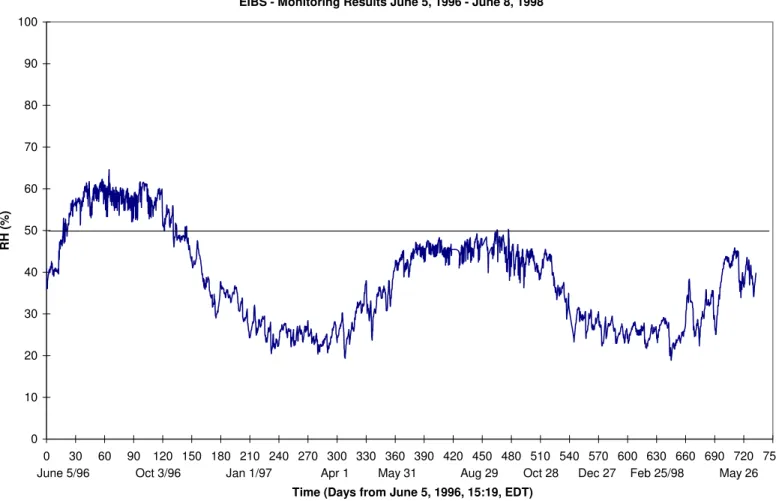
1.4.2 Indoor RH

The indoor RH was also monitored. The outdoor RH varies from dry conditions (e.g. 40%) to wet (e.g. near 100%) on a regular basis, with no significant change from season to season (plot not shown).

Indoor RH 0 10 20 30 40 50 60 70 80 90 100 0 30 60 90 120 150 180 210 240 270 300 330 360 390 420 450 480 510 540 570 600 630 660 690 720 750

Time (Days from June 5, 1996, 15:19, EDT)

RH

(%)

June 5/96 Oct 3/96 Jan 1/97 Apr 1 May 31 Aug 29 Oct 28 Dec 27 Feb 25/98 May 26

(19)

The indoor RH shown in Figure 7 shows a more important trend: the second summer had significantly lower RH in the basement than the first summer. Three possible explanations are:

1. The second summer featured a prolonged period of drought with little rainfall being recorded by Environment Canada from mid-July to late August. As a result, the soil (clay) near the hut was observed to be dry in late August when some digging took place around the hut. As well, the clay was observed to shrink away from the wall, leaving a noticeable gap between the soil and the wall.

2. A related explanation is that with the better weather in the second summer, there would have been more air conditioning (not monitored) and thus potentially more drying of interior air.

3. The sump pump controls were adjusted in January 1997, which progressively lowered the standing water in the sump from about footing height to about 0.5 m below the footing. Could this have caused less moisture to evaporate through the slab?

The potential impact of the dry summer of 1997 and of the sump pump adjustment are probably important since changes in soil moisture content and in specimen performance over these periods coincide with these events.

(20)

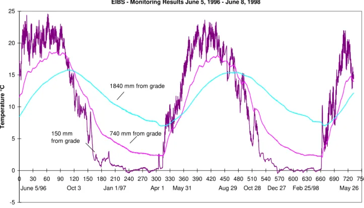
1.4.3 Soil Temperatures

Soil temperatures at three depths are plotted in Figure 8. These were measured at 150 mm, 740 mm and 1840 mm below grade, over two-year period. The shallower sensor shows the greatest variation from summer to winter, and diurnal effects can be observed. no diurnal effects can be seen at the two lower depths. The lowest depth approximates a sine wave.

Soil Temperatures Adjacent to Sample W6

-5 0 5 10 15 20 25 0 30 60 90 120 150 180 210 240 270 300 330 360 390 420 450 480 510 540 570 600 630 660 690 720 750

Time (Days from June 5, 1996, 15:19, EDT)

T e mp eratu re ° C

June 5/96 Oct 3 Jan 1/97 Apr 1 May 31 Aug 29 Oct 28 Dec 27 Feb 25/98 May 26 150 mm

from grade

1840 mm from grade

740 mm from grade

(21)

It should be noted that in both winters, the frost penetrated approximately 150 mm. The frost depth temporarily reached 270 mm in the second winter (not shown in graph). Snow cover, and repeated thaws in both heating seasons are suspected to be the cause. The mostly clay soils also contribute to shallow frost penetration. An independent temperature measurement in the second winter, 10 m from the house showed the same result. This indicates that at 2 m from the house, there is an undetectable effect on soil temperature, for this well insulated basement.

There was also relatively little variation in temperature measured over 5 locations in the soil parallel to the wall (graph not shown).

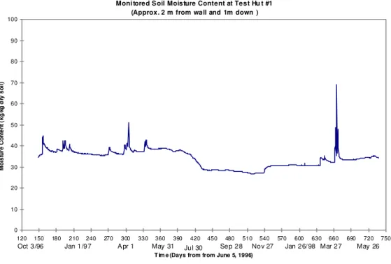
1.4.4 Soil Moisture Content

A single TDR probe (time domain reflectometry) was deployed about 2 m from the east wall and 1 m down into the ground, to monitor soil moisture content on an ongoing basis. Figure 9 presents the results of the soil moisture content monitoring over the period from October 1996 to June 1998. It shows that the soil was wet throughout the first heating season and dried substantially in the summer of 1997. The soil stayed dryer in throughout most of the second heating season than the first, until the spring thaw in 1998.

(22)

Moni tored S oil Moisture Content at Test Hu t #1 (Approx. 2 m from wall and 1m down )

0 10 20 30 40 50 60 70 80 90 100 120 150 180 210 240 270 300 330 360 390 420 450 480 510 540 570 600 630 660 690 720 750

T im e (Days from from June 5, 1996)

M o is tu re C o n ten t ( k g /k g d ry s o il)

Oct 3/96 Jan 1/97 A pr 1 May 31 _{Jul 30} Sep 28 Nov 27 Jan 26/ 98 Mar 27 May 26

Figure 9 Measured Soil Moisture Content over Two Heating Seasons

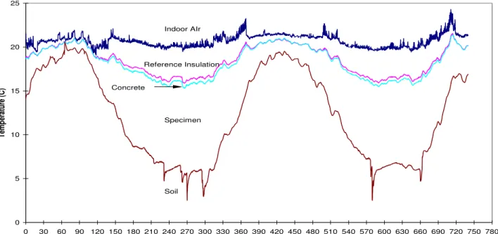
1.4.5 Temperature Profiles Through the Wall at Mid-Height

Figure 10 shows the two-year temperature record at four locations through the wall at specimen W6: the interior surface, both sides of the concrete, and the exterior surface of the specimen in contact with the soil. The inner surface of the wall is kept near 21°C, with small variations throughout the two years. Main control events such as power outages and changes from heating to air conditioning and back are evident from these temperature readings. The temperature at both sides of the concrete are quite close (concrete being a poor thermal insulator), and these vary from 15°C to 20°C, from winter to summer.

(23)

0 5 10 15 20 25 0 30 60 90 120 150 180 210 240 270 300 330 360 390 420 450 480 510 540 570 600 630 660 690 720 750 780

Days from Start

T emp erat ure ( C ) Oct 3/96

June 5/96 Jan 1/97 Apr 1 May 31

Reference Insulation

Concrete

Specimen Indoor AIr

Soil

Jul 30 Sep 28 Nov 27 Jan 26/98 Apr 26 June 25

Figure 10 Temperature Profiles at the Mid-Position of Specimen W6 on the West Wall

The lowest curve in the graph is the temperature record for the insulation/soil interface. These vary between about 5°C in winter up to a maximum of about 20°C in summer.

The periodic ‘spikes’ in this curve correspond to record events of heavy precipitation or winter thaws. The August 8, 1996 rain and flood was a 1 in 75-year event for Ottawa. During this tropical storm, the temperature at the insulation/soil interface deflected upwards, apparently due to warm rainwater moving down the wall. Such deflections were observed at the mid, low and bottom thermocouple positions during the same period, tracing the path of the water. These deflections were much less noticeable at the high position, where the soil temperature would be closer to the temperature of the moving water.

(24)

The deflections in the winter are downward because the melt water temperature is initially 0°C, which would cool the soil and insulation at the interface. In the first year, these deflections were often smaller or absent on the east wall where the ground surface was properly graded outward. The exceptions corresponded to events with driving rain from the east. In the second year, the differences between east and west were less noticeable. A final review of soil slopes near the wall revealed that by the end of the second year, most of the slopes had settled on the east wall. These were now mostly inward, as recorded in figure 11 and figure 12.

Elevation - East Wall

99.95 100.00 100.05 100.10 100.15 0 0.5 1 1.5 2 2.5

Distance from wall in m

El e vat ion i n m E1 E4 E6 E8 Average slope toward wall:

1.3% -3.0%

(25)

Elevation - West Wall 99.95 100.00 100.05 100.10 100.15 0 0.5 1 1.5 2 2.5

Distance from wall in m Ele vati on W1 W4 W6 W8

Average slope toward wall = 6.3%

Figure 12 Final Soil Elevations at the West Wall

1.4.6 Temperature Profiles at all Vertical Locations

Temperature profiles similar to the ones presented in Figure 10 are presented in Appendix B for all vertical locations on wall w6. In these graphs, it can be noted that the vertical deflections in the temperature profile at the insulation/soil interface correspond in time. This strongly suggests the downward movement of water along this interface. These temperature deflections are less apparent or non-existent at the high position for several reasons. Temperatures at this location are closer to freezing in the winter and therefore would not show the movement of water at the same temperature; soil temperatures at this location near the surface also vary more with ambient temperatures. Finally, the thermocouples in this location are covered by the cementitious board (Figure 2), so that water may not be in direct contact with the insulation specimen at this point.

(26)

With the possible exception of the lowest position (50 cm up from the slab), the concrete, which is behind the specimen, generally do not show corresponding temperature deflections during these events. This suggests that the concrete wall is either remaining dry, or less likely, that the water or moisture has heated to equilibrium by the time it reaches the concrete. The deflection of the concrete at the bottom thermocouples opens the possibility that melt-water is reaching the concrete at that point. It is also possible that the footing is being cooled by the melt-water, which in turn cools the concrete wall at that location, due to the thermal bridge of the footing. One specimen (SPF) was sealed to the footing and wall, and it did not show temperature deflections of the concrete during rain/thaw events.

1.4.7 Heat Flux Profiles

Temperature differences across the thermally calibrated insulation layer at the inner face of the wall were calculated at 4 vertical locations with thermocouple and three vertical locations with heat flux meters shown in Figures A1 and A2.

(27)

Example Heat Flux Profiles Into the Basement Wall For October 1996, January and June 1997

0 200 400 600 800 1000 1200 1400 1600 1800 2000 0 1 2 3 4 5 6 7 8 9 Heat Flux (W/m2) Ver

Figure 13 Typical Profiles of Heat Flux through the Reference Insulation at the inner face of the Wall

The smoothness or regularity of these curves attests to the fact that the seven vertical readings are consistent with one another. These weekly averaged heat flux profiles have the highest level of accuracy associated with them. Each heat flux meter reading is the result of the average of 5 EMF readings.

10 tical Dista n ce from Slab (mm) October January June

(Heat flux measured in this direction)

(28)

1.5 Analysis

Examination of preliminary results highlighted difficulties in establishing the precision of thermal testing without addressing 3-D effects. This is best illustrated by comparing W5 and W6 tested wall sections.

Table 1a. Measured temperature, heat flux and temperature difference across the insulation specimen, averaged over the week 9 to 16 December 1996.

Specimen Position W5 W6 Temperature Inside Specimen (°C) Temperature Outside Specimen (°C) Temperature Inside Specimen (°C) Temperature Outside Specimen (°C) Bottom 16.91 14.37 16.78 13.55 Low 17.38 12.30 17.44 11.67 Middle 16.82 9.60 17.14 8.49 High 15.98 5.24 16.47 4.37 Avg. temperature 16.77 10.38 16.96 9.52

Table 1b. Apparent steady-state thermal resistance of specimens W5 and W6 calculated from data shown in Table 1a.

W5 W6

Temp. difference across the wall, oK 6.39 7.44

Mean heat flux on inner surface, W/m2 4.30 4.10

Apparent R-value, (m2 K)/W 1.49 (100%) 1.81(122%)

Table 1 shows average temperature difference across the insulation layer and heat fluxes entering each of these two tested wall sections. Higher temperature of concrete (16.96 oC) behind W6 is the signal for lateral heat flow. These results are averaged over a period of one week to approximate the steady state and use the ratio between the temperature difference and the heat flux as an indicator of thermal resistance. When thermal

(29)

resistance of W5 is taken as a benchmark (100%), the ratio between W6 and W5 specimens is 122%. This result is, however, much lower than the ratio of 164 percent obtained from the initial, laboratory measurements of thermal resistance performed on specimens W5 and W6. Even if the R-value of W6 specimen was corrected for the effect of foam aging, the difference between one-dimensional estimate and the measured results is significant. This difference highlights the need for 3-D model application.

1.6 Discussion

As the test set-up involved diverse thermal insulating materials placed next to each other, the presence of lateral heat flow was inevitable. In the case of specimen W6 (closed-cell, gas-filled thermal insulating foam), some heat would be conducted laterally through the concrete wall and pass through the adjacent specimen, which has a lower thermal resistance. The lateral heat flow may explain that the ratio of estimated thermal resistance of two adjacent specimens W5 and W6, shown in Table 1, is smaller than the ratio indicated by the laboratory comparison.

To evaluate effects of lateral heat flow on the precision of the field measurements, a new task was added to the EIBS project, namely development of a 3-D model. The first question was then, how to discretise the continuous equations to arrive at the system, which is easy to solve with numerical techniques.

(30)

2. Heat Transfer Model

The aim of this study is to determine the in-situ thermal performance of basement insulation specimens placed on the exterior of the wall. We developed a method for studying the thermal behavior of different constituent layers of the wall and to assess the thermal properties of the specimens (conductivity and heat capacity).

Our work is focused on the exterior insulation of basement. We intend to analyze one wall with three components:

• First layer (interior) : reference • Second layer : concrete

• Third layer (exterior): insulation.

We consider in this study consider only the conduction heat transfer in the wall, by specifying a control volume at the outer thermocouple boundary. The comparison of our model with experiment data will validate its application.

This section specifies the model for heat transfer, based on principles of conduction heat transfer.

2.1 Analysis and Discussion

2.1.1 Method to Measure Thermal Resistance In Situ

A test method, developed at NRC during previous project (Muzychka, 1992; Bomberg and Kumaran 1994) [10-11], involves testing two materials placed in contact with each other - a reference material whose thermal conductivity and specific heat are known as a

(31)

function of temperature, and a test specimen whose thermal properties are unknown. Because of its comparative character, this method has been called a heat flow comparator (HFC). In a previous experiment involving roof insulation, the reference and tested specimens were placed in the exposure box representing a conventional roofing assembly. Thermocouples were placed on each surface of the standard and reference materials to measure temperatures, which then were used as the boundary conditions in the heat flow calculations.

The heat flux across the boundary surface between reference and tested specimen is calculated using a numerical algorithm to solve the heat transfer equation through the reference material. Imposing the requirement of heat flux continuity at the contact boundary between test and reference materials, corresponding values of thermal conductivity and heat capacity of the tested specimens are found with an iterative technique. Performing these calculations for each subsequent data averaging period will result in a set of thermal properties of the test material which, over the period of measurements, give the best match with its boundary conditions (temperatures and heat flux).

Since thermal conductivity of the specimen is a function of its temperature, the solution of the heat transfer equation is based on central finite difference calculations that include Kirchoff's potential function (integral of thermal conductivity over the range of temperature) and uses a Taylor's series to calculate heat flux through the surface. Subsequent developments improved the stability of the numerical solution and produced a user friendly computer code that includes optimization routines. This method was

(32)

documented and applied for determining the in-situ thermal resistance of roof insulation (Bomberg and Kumaran, 1994) [10]

2.1.2 Dimensional Analysis

The analysis technique for EIBS study was adapted to account for two significant differences in the test set-up:

1. The 200 mm concrete wall was interposed between the reference insulation layer and the test specimen. Analysis showed that the concrete layer modifies the heat flux leaving the reference specimen through heat storage and through heat flow up and along the concrete wall.

2. Temperatures in the soil did not vary significantly on a diurnal basis, so that a statistically valid relationship between specimen conductivity and temperature was not needed to the extent considered for the roofing specimens.

The analysis was therefore adapted to assess the heat storage effects and two dimensional heat losses through and up the wall. A second, more elaborate method was developed to assess the heat loss in the third dimension, along the wall, and to suggest what corrections to the 2-D results would be needed.

The 2-D analysis consisted of calculating the horizontal heat flux (inside to outside) and vertical heat flux (bottom to top) through all materials in the control volume defined in Appendix C. A finite difference technique was used to solve the heat transfer equations for dynamic heat flow through solids with known boundary conditions, at each point of a nodal network used to represent the materials in the control volume (see Appendix C).

(33)

Using this analysis technique, the temperature differences across the specimen and the concrete were calculated for each measurement interval. The temperature difference across the reference insulation determines the heat flux into the concrete. Finite difference analysis was used to assess the direction and magnitude of heat flux in the concrete as well as the amount of heat stored or released by the concrete. After these quantities are evaluated through the concrete, the resulting net heat flux into the specimen was assessed. Using this heat flux and a postulated thermal conductivity of the specimen, the resultant temperature differences across the specimen were calculated. The calculated temperature differences are then compared to measure results, every ten minutes. Mean errors were calculated on a weekly basis. An iterative technique was devised to minimize the mean error between calculated temperature differences and measured, by adjusting the postulated conductivity of the insulated specimen on a weekly basis.

The factor by which the conductivity was adjusted relative to lab-determine conductivity of the specimens was labeled ‘conductivity adjustment factor’. These were recorded and plotted on a weekly basis. As well as the reciprocal – the thermal resistance adjustment factors was plotted. As a final step in the analysis process, the adjustment in thermal resistance of the specimen as normalized to an initial average adjustment for October 1996 – the first period of cold weather in the monitoring period.

2.1.3 Assessment of 3-Dimensional Heat Flow

Over the course of the 2-dimensional analysis, it was noted that the temperature of the concrete (behind the specimens) differed from specimen to specimen. This raised the possibility that heat could flow through the concrete from one specimen to another, resulting in possible uncertainty in the orders of magnitude of performance assessed using the 2-dimensional analysis.

(34)

In response to this, a detailed 3-dimensional heat transfer analysis of the both the east-wall and the west wall were undertaken. The same control volume depicted in appendix C was used for the 3-D analysis, but this was extended in the third dimension along the wall, to encompass all specimens. The objective of this much more detailed analysis was to determine the order of magnitude of lateral heat flow in the concrete from one specimen to another, and to provide a correction on the 2-dimensional results for in-situ R-value of each specimen, where needed. To illustrate the result of this analysis, an example result is shown appendix D for the west wall. The angle between the actual heat flux vector and the normal direction is defined here as the heat flux angle; e.g. a zero angle denotes heat flux normal to the wall -–no lateral heat flow. The heat flow angle is plotted for the ‘top’ location (top of the control volume) in the concrete, at one point in time. A positive angle means lateral heat flow towards one end of the wall, and a negative heat flow means lateral heat flow towards the other.

The significance of this diagram is as follows. If the flow angle in the concrete behind the specimen is small, and in the same direction, then the lateral heat flow has little effect on the results. This was the case for W2, W3, W4, W5 and W8. On the other hand, specimen W6 appears to have been affected by significant lateral heat flow. Starting at the center of the specimen, the heat flow on the south side is flowing south and the heat flow on the north side is flowing north. This is thus a lateral heat drain from the specimen, causing us to underestimate its thermal performance in the 2-D analysis. With this lateral flow, specimen W7 is gaining heat from W6, but is not passing this onto W8. The 2-D analysis would overestimate its performance for this point in time, at this vertical location of the specimen.

(35)

These lateral heat flows varied according to vertical position in the specimen and with time. The results were thus integrated over full height of the specimen and over each of two heating seasons. The 3-D analysis thus confirmed the order of magnitude of performance for specimens W2, W3, W4, W5, W7 and W8. The lateral heat flows affected specimen W6 in a significant way. The 3-D analysis showed better thermal performance of the W6 specimen in than the 2-D analysis by about 10%.

The current report presents the 2-D analysis results, reported in terms of thermal resistance relative to an initial condition

2.2 State of the art of analytical techniques

There are a number of numerical models available for this kind of study.

Bhattacharya M.C. [12] and Lick W. [13] applied the improved finite-difference method (FDM) to time-dependent heat conduction problems with step-by step computation in the time domain. The finite-element method (FEM) based on variational principle was used by Gurtin M.E. [14] to analyze the unsteady problem of heat transfer. Emery A.F. and Carson W.W. [15] and Visser W [16]. applied variational formulations in their finite-element solutions of nonstationary temperature distribution problems. Bruch J.C. and Zyvoloski G. [17] solved the transient linear and non-linear two-dimensional heat conduction problems using the finite-element weighted residual process. Rources V.E. and Alarcon E. [18] presented a formulation for a two-dimensional isotropic continuous solid using the boundary integral equation method (BIEM) with a finite-difference approch in the time domain. Chen et al [19] successfully applied a hybrid method based on the Laplace transform and the FDM to transient heat conduction problems.

(36)

The disadvantages of these methods are the complicated procedure, need for large storage and long computation time. Wang et al [20] used the implicit spline method of splitting to solve the two and three-dimensional transient heat conduction problems. The method is applied to homogeneous and isotropic solid.

A cubic spline method has been developped in the numerical integration of partial

differential equations since the pioneering work of Rubin and Graves [21], and Rubin and Khosla [22]. This method provides a simple procedure, small storage, short computation time, and a high order of accuracy. Furthermore, the spline method has a direct

representation of gradient boundary condition.

In this study, an implicit spline method is used for solution of three-dimensional transient heat conduction problems for a non-homogeneous medium.

2.2.1 General principal

Heat propagation in a solid medium is governed by the heat conduction equation:

( )

_{( )}

) 1 2 ( , , , − + ∇ ∇ = ∂ ∂ t X Q t X T t t X T C λ ρ With:

X (x,y,z): coordinates in the 3 directions. T (X, t): temperature at time t. [K] λ : thermal conductivity. [W/m.K]

(37)

ρ : density. [kg/m3

]

C: heat capacity. [J/kg. K]

Q (X, t): internal heat generator per unit of volume. [W/m3]

Some assumptions are considered: • thermal conductivity is constant,

• no chemical reaction, no dissipation of internal energy in the wall, e.g. no phase change inside the wall,

• homogeneous isotropic medium (concrete, insulation).

Taking into the account the hypothesis, equation (2-1) is reduced to:

⎟⎟ ⎠ ⎞ ⎜⎜ ⎝ ⎛ ∂ ∂ + ∂ ∂ + ∂ ∂ = ∂ ∂ ∇ = ∂ ∂ 2 2 2 2 2 2 2 z T y T x T a t T or T a t T (2-2) where

[

m /2 s

]

C a ρ λ

= : thermal diffusivity of the medium

This equation, with suitable boundary and initial conditions, represents the temperature distribution at any time and at any point in the volume, under consideration.

(38)

In real situations, temperature-dependent coefficients

(

λ,ρ,C

)

should be taken into account. The temperature dependence of heat capacity and thermal conductivity has an important effect on heat transfer in high-temperature processes. Such temperature-dependent coefficient lead to non-linear heat-conduction problems.

The finite-difference techniques are suitable for this kind of problems, because it conserves a good physical significance to the different parameters whose it appears.

Finite-difference method used classically to solve heat transfer equations, results in one spatial discretisation and one temporal discretisation. This method is practically the only method applicable to non-linear problems.

The electric analogy can help for clarification of good representation of problem of conduction heat transfer.

2.2.2 Definition of the analogy “Thermal phenomena/electric phenomena”

There is taken essentially into correspondence between electric and thermal variables whose we are summarizing in the table 1 (Maref, 1992) [23]:

Table 1: The Thermal / Electric analogy

Thermal variables Electric variables

Temperature Potential

Heat flux Intensity

Thermal conductivity Electric conductance

(39)

2.2.3 Application of the electric analogy to the 1-D conductive model

The electric analogy leads, after spatial discretisation of the problem (nodal method), to an electrical network. This discretisation handles the different spatial variables and permit to transform the partial differential equations to algebrair-differencial equations.

Figure 14: 1-D conductive Model of homogenous wall and its equivalent electric network With ⎪ ⎪ ⎩ ⎪ ⎪ ⎨ ⎧ = = = = = = = = Δ = = = Δ = − − R K K K R R R R x R R R C x C n n n n S S m i / 1 . ... ... .. ... ... 2 / 2 / . . , 1 23 12 , 1 23 12 2 1 λ ρ Where ⎪ ⎪ ⎩ ⎪ ⎪ ⎨ ⎧ Δ ce Conduc K j node the and i node the between ce sis R m tion discretisa spatial of step x K kg J material of capacity heat C j i j i m tan : tan Re : ) ( : ) . / ( : , ,

(

)

tion discretisa temporal the is t where t n t time at i node at e temperatur a be T Let _in Δ Δ + = + , , θ θ

(40)

(

)

(

)

⎪ ⎩ ⎪ ⎨ ⎧ ≤ ≤ − + − = ⎟⎟ ⎠ ⎞ ⎜⎜ ⎝ ⎛ ∂ ∂ ₊ ₊ + + + + − − + 1 0 1 1 , 1 , 1 θ θ θ θ θ θ n i n i i i n i n i i i n i i K T T K T T t T C (2-3) 2.2.4 Finite-Difference Method

The KIRCHOFF law is written for each node i, at time step Δt:

( )

n 1 t, for 1 (Implicitscheme)

t= + Δ θ =

(

)

(

)

(

1 1 1 1 , 1 1 1 , 1 1 + + + + + + − − + ₋ ₌ ₋ ₊ ₋ Δ n i n i i i n i n i i i n i n i i T T K T T K T T t C

)

(2-4)

2.2.5 Construction of Thermal Conductivity Matrix

KIRCHOFF law applied to the discretised system permit to write the conductivity Matrix [A]. (Mokhtari A.M., 1988) [24].

Note: We have chosen the convention: concerning the interior node location of the wall: The origine (node (0,0,0)) is located at the north, innermost corner of the wall with 1 to n, both for the east and west wall.

(41)

2.2.5.1 Boundary condition 2.2.5.1.1 First kind (Dirichlet)

Figure 15

A temperature applied over the wall surface characterized the boundary condition of the first kind. The energy balance at the node 1 is written as:

(

)

(

) (

1 1 1 2 1 1 1 1 1 1 1 + − =₂ + − + + + − + Δ n n n n se n n T T K T T K T T t C

)

(2-5) Then ⎟ ⎠ ⎞ ⎜ ⎝ ⎛ ₊ Δ − = + ⎟ ⎠ ⎞ ⎜ ⎝ ⎛ ₊ Δ − + + +1 1 1 1 2 1 1 1 2 3 sen n n n KT T t C KT T K t C (2-6) With:

( )

K A K t C A R K = ⎟ ⎠ ⎞ ⎜ ⎝ ⎛ ₊ Δ − = = 2 , 1 3 1 , 1 1 1

(42)

2.2.5.2 Thermal Balance at the Current Node Ti - 1 Ti Ti + 1 Figure 16 n i i n i n i i n i T t C KT T t C K KT Δ − = + ⎟ ⎠ ⎞ ⎜ ⎝ ⎛ Δ + − + + + + − 11 1 1 1 2 (2-7) With:

( )

(

i i

)

K A K t C i i A i = − ⎟⎟ ⎠ ⎞ ⎜⎜ ⎝ ⎛ + Δ − = 1 , 2 ,

2.2.5.3 Thermal Balance close by two layers

T T T T

φ φ

(43)

Assuming a perfect contact , φ12 = φ21, the following equation are obtained:

(

)

(

1

)

' 2 2K T_i −T_c = K T_c −T_i₊ ' 1 ' K K T K KT T i i c + + = + (2-8) At node i

(

1 1

)

(

1 1 1 1 2 + + + + − + − + − = ⎟⎟ ⎠ ⎞ ⎜⎜ ⎝ ⎛ ∂ ∂ _n i n c n i n i n i i K T T K T T t T C

)

(2-9)

After rearranging, equation (2-9) is reduced to

1 1 ' ' 1 ' ' 1 1 1 2 3 + + + + − + ⎟⎟ ⎠ ⎞ ⎜⎜ ⎝ ⎛ + + ⎟⎟ ⎠ ⎞ ⎜⎜ ⎝ ⎛ + + − = ⎟⎟ ⎠ ⎞ ⎜⎜ ⎝ ⎛ ∂ ∂ n i n i n i n i i T K K K K T K K K K K KT t T C 1 2 ' 1 1 ' ' 1 ' ' 1 1 3 ' 2 + + + + + + + + ⎟⎟ ⎠ ⎞ ⎜⎜ ⎝ ⎛ + + − + = ⎟⎟ ⎠ ⎞ ⎜⎜ ⎝ ⎛ ∂ ∂ _n i n i n i n i i T K T K K K K K T K K KK t T C (2-9 bis) At node i+1 Posing factor Interface as K K K K E_i ' ' + − =

We rewrite the balance at node i and i+1 function of the interface factor. At node i

(

)

[

(

)

(

)

1

]

1 1 1 1 1 1 2 + ₊+ + − + ₋ ₌ ₊ ₋ ₊ ₋ Δ n i i n i i n i n i n i i T E T E T K T T t C (2-10) At node i+1

(44)

(

)

[

(

)

(

)

1

]

1 1 1 1 ' 1 1 1 1 2 + − + + + + + + − = + − + + Δ n i n i i n i i n i n i i T T E T E K T T t C (2-11) Note:

(

Ei

)

K

(

Ei K' 1+ = 1−

)

(2-12)

2.2.5.4 Thermal Balance at the last node The equation will be written as:

⎟⎟ ⎠ ⎞ ⎜⎜ ⎝ ⎛ + Δ − = ⎟⎟ ⎠ ⎞ ⎜⎜ ⎝ ⎛ + Δ − + + + −11 ' 1 ' 1 ' 2 3 n i _in _sin i i n i T K T t C T K t C T K (2-13)

For the first kind of thermal link, 7 nodes (4 in the first layer and 3 in the second) will represent the thermal conductivity Matrix for discretised system.

[ ]

(

)

(

)

(

)

(

)

(

) ( )

( )

(

)

(

)

(

)

(

)

⎟⎟ ⎟ ⎟ ⎟ ⎟ ⎟ ⎟ ⎟ ⎟ ⎟ ⎟ ⎟ ⎟ ⎟ ⎟ ⎟ ⎟ ⎟ ⎟ ⎠ ⎞ ⎜⎜ ⎜ ⎜ ⎜ ⎜ ⎜ ⎜ ⎜ ⎜ ⎜ ⎜ ⎜ ⎜ ⎜ ⎜ ⎜ ⎜ ⎜ ⎜ ⎝ ⎛ Δ − − Δ − − + − Δ − + − Δ − − Δ − − Δ − − Δ − − = t C k k k t C k k k E k t C E k E k t C E k k k t C k k k t C k k k t C k A / 3 / 2 2 / 1 1 / 2 / 2 / 2 / 3 2 ' ' ' 2 ' ' ' 2 ' 2 1 ' 1 1 1 1 1 1

(45)

3. Heat conduction in Three Dimensions

3.1 Thermal conductance

Figure 5 shows a cell (i, j, k) with the side lengths Δx , Δy and Δzi j k. There are six

adjacent cells. The figure shows the cell (i, j, k+1) located directly above.

The heat flow Qi, j, k + 1(W) from cell (i, j, k) to cell (i, j, k+1) is given by the conductance

multiplied by the temperature difference between these two cells:

(

T T

)

( )

W

K

Q_i_,_j_,_k₊₁_/₂ = _i_,_j_,_k₊₁_/₂ _i_,_j_,_k − _i_,_j_,_k₊₁ (3-1)

Where Ki, j, k+1/2, (W/K), is the conductance between two cells (i, j, k) and (i, j, k+1). The

other five heat flows pertaining to cell (i, j, k) are calculated in the same way.

Δzk

Δyj

Δxi

Ti, j,k + 1

Ti, j,k

(46)

Ti– 1, j, k Ti, j, k Ti + 1, j, k Ti, j, k + 1 Ti , j +1, k Ti, j, k - 1 Ti, j -1, k Rj-1 Rk Rk+1 Ri Ri+1 Rj+1 Figure 19

The conductance Ki, j, k+1/2, (W/K), between the two cells (i, j, k) and (i, j, k+1) is

calculated as:

(

) (

)

(

W K r z z y x K k j i k j i k k j i k j i k j i / 2 2 _, _, ₁ , , 1/2 1 , , 2 / 1 , , + + + + + Δ + Δ

)

Δ Δ = λ λ (3-2)

Where λi, j, k , (W/(m.K)), is the thermal conductivity at cell (i, j, k). The conductance

refers to the total heat flow through the area Δx Δyi j. The first term in the denominator is

the thermal resistance in the z-direction for half of the cell (i, j, k), The second term being the resistance for half of cell (i, j, k+1). The third term, ri, j, k+1/2, is an optional additional

(47)

thermal resistance at interface between the two cells (i, j, k) and (i, j, k+1). We assume a perfect contact; that this resistance is equal to zero.

Equation (3-2) is valid for all internal cells (an internal cell has at least one cell on each side). For boundary cells, the equation is modified in the following way. Consider cell (1, j, k) that lies at the boundary. The conductance, which couples the temperature Ti, j, k with

a boundary temperature is:

(

)

(

W K x z y K k j i k j k j / 2 ₁_, _, , , 2 / 1 λ Δ

)

Δ Δ = (3-3)

3.2 Heat flows

An energy balance is calculated for each cell. The total heat flow to cell (i, j, k) from the six adjacent cells is put in the variable Hi, j, k (W):

(

)

(

)

(

)

(

)

(

1 , , 1 1 , , 2 / 1 , , 1 , , 1 1 , , 2 / 1 , , 1 , , 1 , 1 , , 2 / 1 , 1 , , 1 , 1 , , 2 / 1 , 1 , , 1 , , 1 , , 2 / 1 1 , , 1 , , 1 , , 2 / 1 , , + + + + + + − − + + + + + + − − + + + + + + − − − + − + − + − + − + − = n k j i n k j i k j i n k j i n k j i k j i n k j i n k j i k j i n k j i n k j i k j i n k j i n k j i k j i n k j i n k j i k j i k j i T T K T T K T T K T T K T T K T T K H

)

(3-4)

The increase of the energy for an internal cell during time-step Δt is given by the energy balance below.

(

)

i jk n k j i n k j i k j i k j i H T T z y x t C , , , , 1 , , , , _Δ _Δ _Δ ₋ ₌ Δ + (3-5)

, (J/m3K), is the volumetric heat capacity. Where Ci, j, k

(48)

(

) (

)

(

, , 1/2 , , 1/2

)

, 2 / 1 , , 2 / 1 , , , 2 / 1 , , 2 / 1 , , 1 , , , , + − + − + − + − + − + − = − Δ Δ Δ Δ k j i k j i k j i k j i k j i k j i n k j i n k j i k j i k j i Q Q Q Q Q Q T T z y x t C (3-6)

The advantage of the introducing the Hi, j, k variable is that less data need to be collected

in computer memory.

The arrays that are needed in the three-dimensional case are normally eight:

2 / 1 , , , 2 / 1 , , , 2 / 1 2 / 1 , , , , 2 / 1 , , , 2 / 1 , , , ,jk i jk i+ jk i j+ k i jk+ i+ jk i j+ k i jk+ i C K K K Q Q Q T

variable gives instead six three dimensional arrays: Introducing the Hi, j, k k j i k j i k j i k j i k j i k j i C K K K H T_, _, _, _, ₊₁_/₂_, _, _, ₊₁_/₂_,_, _, _, ₊₁_/₂ _, _,

Three of the products (conductance multiplied by temperature difference in Eq. (3-4)) have to be calculated at each time step. This may save almost half the computer time compared with the direct use of Eq. (3-4). The following procedure, which is used for all internal cells (i, j, k), illustrates this (Blomberg, 1996) [25]. Three local variables, Q , Qx y

and Qz, are introduced in order to decrease the number of arithmetic operations. The heat

flows from the three cells “upstream” (i+1, j, k), (i, j+1, k), and (i, j, k+1) to cell (i, j, k) are put in variables:

(

)

(

i jk i jk

)

k j i k j i k j i k j i k j i k j i k j i T T K Q T T K Q T T K Q z y x , , 1 , , 2 / 1 , , , , , 1 , , 2 / 1 , , , , , 1 , , 2 / 1 − = − =

)

− = + + + + + + (3-7)

The change in heat for the cells “upstream” is directly made as

z y x Q H H Q H H Q H H n k j i n k j i n k j i n k j i n k j i n k j i − = − = − = + + + + + + + + + 1 , , 1 1 , , , 1 , 1 , 1 , , , 1 1 , , 1 (3-8)

(49)

z y x Q Q Q H H_in_,+_j1_,_k = _in_,_j_,_k + + +

The final equation for the new temperature becomes:

1 , , , , , , 1 , , + + Δ Δ Δ Δ + = n k j i k j i k j i n k j i n k j i H z y x C t T T (3-9)

The time-step Δt for cell (i, j, k) is determined using the following stability criterion:

k and j i all for K z y x C t i,j,k i j k , ,

∑

Δ Δ Δ Δ p (3-10) where 2 / 1 , , 2 / 1 , , , 2 / 1 , , 2 / 1 , , , 2 / 1 , , 2 / 1 + − + − + − + + + + + =

∑

K Ki jk Ki jk Ki j k Ki j k Ki jk Ki jk (3-11)

This criterion must be satisfied for cells (i, j, k). The smallest stable time-step obtained is used for all cells to guarantee stability.

4. Computational algorithm

Real heat transfer processes take place in three-dimensional patterns. Three-dimensional effects should be accounted for as much as possible in the analysis of heat-conduction problems. However, the solution of three-dimensional problems requires a considerable computational work.

The difficulties involved in shifting from one-dimensional to two-dimensional problems are compounded when one attempts to solve three-dimensional problems. This results in an increase in the computation time of more than an order of magnitude, as compared with the two-dimensional case.

However, in such cases, because of three-dimensionality and stability, additional difficulties are normally encountered. Care should therefore be exercised in choosing an

(50)

appropriate finite difference scheme, since the number of operations involved may be beyond reasonable limits.

The numerical stability of the finite difference scheme is also a problem in the case of two or more dimensions. This, however, applies only to very simple computational procedures.

The calculation of , with known, requires a number of arithmetic operations proportional to the number of unknown quantities. Therefore, the explicit scheme cannot be optimal, and it is stable only with very limitations on time steps. The application of explicit procedure to two-dimensional and multidimensional problems may often not be practical, because of the very severe limitations on the time steps. However, two methods of resolution are considered: Splitting-step method and Spline method.

1 , , + n k j i θ n k j i, , θ

4.1 Splitting-step method.

Difference procedures based on fractional steps have been used to solve multidimensional problems. The procedures combine the advantages of explicit and implicit schemes: they are certainly stable, and the transition from one step to the next requires a number of arithmetic operations proportional to number of the grid points. The economy of different procedures based on the fractional-step method results from the fact that the multidimensional problems can be reduced to one-dimensional cases, with the later being solved by the factorization method. It is known as the splitting-step method. Consider a three-dimensional problem written in operator form as

T L T L T L t T z y x + + = ∂ ∂ (4-1)

(51)

Where are the differential operators z L and y L x L ,

(

)

x T t z y x k x T L_x ∂ ∂ ∂ ∂ = ₁ , , ,

(

)

y T t z y x k y T L_y ∂ ∂ ∂ ∂ = ₂ , , , (4-2)

(

)

z T t z y x k z T L_z ∂ ∂ ∂ ∂ = ₃ , , ,

The solutions T

(

x,y,z,t

)

is sought inside the parallelepiped 0≤x≤l_x, 0≤ y≤l_y,

z l

z≤

≤

0 , with the boundary conditions

(

x y z t

)

(

x y z t

)

T , , , _Γ =φ , , , (4-3)

0 =

t

In addition, the temperature distribution in the parallelepiped at the initial time is known:

(

x y z

)

(

x y z t

)

T , , ,0 =ψ , , , (4-4)

(

x y z t T , , ,

)

is to be determined for tf0. J l x= _x Δ ,

For the numerical solution of eqs. (4-1)-(4-4), a difference grid using steps

I l y= _y

Δ , Δz=l_z K and is taken for variables x, y, z and t, respectively. The operator , , and

t

Δ

x

L L_y L_z are approximated to the second order of accuracy.

(

)

k j i k j i k j i n k j i n k j i H z y x C t T T , , , , , , 1 , , 1 Δ Δ Δ = Δ − + (4-5) And T L T L T L t T z y x + + = ∂ ∂ (4-6)

Three-dimensional numerical analysis technique for interpreting monitored result of the exterior insulation basement systems (EIBS) experiment

NRC Publications Archive

Archives des publications du CNRC

T hre e -Dim e nsiona l N um e ric a l Ana lysis

Te chnique for I nt e r pre t ing M onit ore d

Re sult of t he Ex t e rior I nsulat ion

Ba se m e nt Syst e m (EI BS) Ex pe rim e nt

M a r e f , W . ; S w i n t o n , M . C . ;

B o m b e r g , M . T . ; K u m a r a n , M . K . ;

N o r m a n d i n , N . ; M a r c h a n d , R . G .

I R C - I R - 8 1 4

September 14, 2000

Table of Contents

Three-dimensional Numerical Analysis Technique for

Interpreting Monitored Results of the Exterior Insulation

Basement Systems (EIBS) Experiment

Abstract

Nomenclature

Three-dimensional Numerical Analysis Technique for

Interpreting Monitored Results of the Exterior Insulation

Basement Systems (EIBS) Experiment

Background

1. Experimental Approach

1.2

Data acquisition

1.3

Duration of the experimental program

1.4

Experimental Data

1.5 Analysis

1.6

Discussion

2. Heat Transfer Model

2.1 Analysis and Discussion

2.2

State of the art of analytical techniques

( )

( )

( )

[

]

(

)

(

)

(

)

(

)

( )

(

)

(

)

(

)

(

)

(

) (

)

( )

( )

( )

(

)

(

)

(

)

(

)

(

)

(

)

[

(

)

(

_{( )}

_{( )}