Correctness of vehicle control systems a case study

Correctness of Vehicle Control Systems:

A Case Study

by

Henri B. Weinberg

B.S., Computer Science

Yale University, 1992

Submitted to the Department of

Electrical Engineering and Computer Science

in partial fulfillment of the requirements for the degree of

Master of Science in Electrical Engineering and Computer Science

at the

MASSACHUSETTS INSTITUTE OF TECHNOLOGY

February 1996

©

Massachusetts Institute of Technology 1996. All rights reserved.

Author ...

Certified by...

...

.

...

...

/

7

Nancy A. Lynch

Professor of Computer Science and Engineering

Thesis Supervisor

Accepted by ...

Chairma

rederic R. Morgenthaler

e on Graduate Students

. OFASSAGHUSETS INSTOLO UiE

OF TECHNOLOGY

APR

111996

LIBRARIES

Correctness of Vehicle Control Systems: A Case Study

by

Henri B. Weinberg

Submitted to the Department of Electrical Engineering and Computer Science on February 5, 1996, in partial fulfillment of the

requirements for the degree of

Master of Science in Electrical Engineering and Computer Science

Abstract

A hybrid system is one in which digital components and analog components

inter-act. Typical examples of hybrid systems are real-time process-control systems such as automated factories or automated transportation systems, in which the digital components monitor and control continuous physical processes in the analog compo-nents. The computer science community has developed formal models and methods for reasoning about digital systems, while the control theory community has done the same for analog systems. However, systems that combine both types of activity appear to require new methods. The development and application of such methods is an active area of current research.

One of the formal tools that has been developed is the hybrid I/O automaton (HIOA) model [1]. In this case study, we show how this model can be used to spec-ify and verspec-ify part of an automated transportation system - a vehicle deceleration maneuver. We investigate how techniques such as automata composition, invariant assertions, and simulation mappings can be applied to systems of communicating dig-ital and analog components. The purpose of the case study is to test the applicability of these computer science based techniques to the area of automated transit. In par-ticular, we are concerned that HIOA techniques express hybrid systems faithfully and that they allow clear and scalable proofs of significant properties of these systems.

In the deceleration maneuver, digital controller slows a train to a target velocity range within a given distance. We examine four versions of the deceleration maneuver, each with a different model of the communication between controller and train: plain, delay, feedback, and feedback with delay. For each case we give a model of the non-controller portion of the system, define correctness of a non-controller, give an example of a correct controller, and prove that it is correct. This case study contains full proofs of the correctness of the various controllers. However, some of the proofs are only sketched, when similar formal proofs appear in other chapters.

Thesis Supervisor: Nancy A. Lynch

Acknowledgments

Thesis supervisor seems a title too antiseptic for Nancy Lynch who gave so generously of herself in the effort to produce this thesis. I have grown and learned under her guidance more than these pages can tell. She and the members of her Theory of Distributed Systems group provided the friendly and stimulating environment that fostered my work. I am especially grateful to Victor Luchangco, Anna Pogosyants, and Rainer Gawlick for their daily advice, support, and friendship.

My research is supported in part by a National Science Foundation graduate fellowship.

I would like to thank my family - _{my parents, Emil and Caroline, my brothers,} Misha and Peter, and above all, my wife, Meg - for their unswerving belief in me.

Contents

1 Introduction 15

2 Model: Hybrid I/O Automata 21

2.1 Trajectories . . . . 21

2.2 Hybrid I/O Automata ... 23

2.3 Hybrid Executions ... 24

2.4 Hybrid Traces ... 26

2.5 Simulation Relations ... 26

2.6 Parallel Composition and Hiding . ... . 27

2.7 Standard HIOA Notation ... 28

2.8 MMT Specifications ... 29

3 Deceleration Case 1: No Delay and No Feedback 37 3.1 Param eters . . ... .. . .. .. .. ... .. .. .. . ... .. .. . 38

3.2 The TRAIN Automaton ... 39

3.3 Properties of TRAIN . ... . . ... 39

3.4 Definition of Controller Correctness . ... 42

3.5 Example Controller: ONE-SHOT ... 43

3.6 Correctness of ONE-SHOT ... 45

3.6.1 Tim eliness . . . 46

3.6.2 Safety . . . .. . 50

4 Deceleration Case 2: Delay and No Feedback 53 4.1 The BUFFER Automaton ... 53

4.3 4.4 4.5

Parameters, Revisited ...

Example Controller: DEL-ONE-SHOT . . . .

Correctness of DEL-ONE-SHOT ...

4.5.1 Non-Violation ... 4.5.2 Timeliness and Safety ...

5 Deceleration Case 3:

Feedback and No Delay

5.1 The SENSOR-TRAIN Automaton ... 5.2 Properties of SENSOR-TRAIN ...

5.3 Definition of Controller Correctness, Revisited 5.4 Parameters, Revisited.. ...

5.5 Example Controller: ZIG-ZAG ... 5.6 Correctness of ZIG-ZAG ...

5.6.1 Timeliness ...

5.6.2 Safety . . . .

6 Deceleration Case 4:

Delay and Feedback

6.1 The ACC-BUFFER Automaton ...

6.2 Definition of Controller Correctness, Revisited 6.3 Parameters, Revisited ...

6.4 Example Controller: DEL-ZIG-ZAG ...

6.5 Correctness of DEL-ZIG-ZAG . . . . 6.5.1 Non-Violation ... 6.5.2 Timeliness .. . . . . 6.5.3 Safety . . . . 7 Conclusion 55 55 56 56 57 63 . . . . 63 . . . .. .. 64 . . . . . 65 . . . . 66 . . . . 67 . . . . 69 . . . . 69 . . . . 73 77 . . . . 78 . . . . . 79 . . . . 79 . . . . 80 . . . . . 82 . . . . 82 . . . . . 84 . . . . 88

List of Figures

3-1 Overview of Basic Deceleration Model . . . .

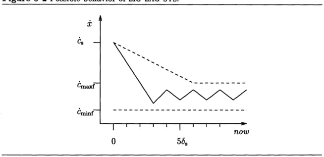
3-2 Example Execution of ONE-SHOT-SYS . . . . Overview of Delay Deceleration Model . . . . Comparison of ONE-SHOT-SYS and DEL-ONE-SHOT-SYS.. Overview of Simulation Mapping . . . . 5-1 Overview of Feedback Deceleration Model . . . . 5-2 Possible behavior of ZIG-ZAG-SYS. . ...

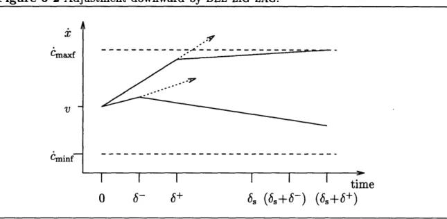
Overview of Feedback with Delay Deceleration Model . . Adjustment downward by DEL-ZIG-ZAG . . . . .

Adjustment upward by DEL-ZIG-ZAG . . . . .

4-1 4-2 4-3 . . . . . 37 . . . . . 45 6-1 6-2 6-3 . . . . . 63 . . . . . 68 . . . . . 78 . . . . . 81 . . . . . 82

List of Tables

The SKEW-TIMER automaton. ... The PING-PONG MMT-specification . ... The hybrid(PING-PONG) automaton.. . . . . The TRAIN automaton ...

The ONE-SHOT automaton (MMT-specification) 4.1 The BUFFER automaton. . ...

5.1 The SENSOR-TRAIN automaton. . ... 5.2 The ZIG-ZAG automaton. . ... 6.1 The ACC-BUFFER automaton.

2.1 2.2 2.3 3.1 3.2 . . . . 30 . . . . 33 . . . . 34 . . . . 40 . . . . . 44 . . . . . 64 . . . . . 67

Chapter 1

Introduction

A hybrid system is one in which digital components and analog components inter-act. Typical examples of hybrid systems are real-time process-control systems such as automated factories or automated transportation systems, in which the digital components monitor and control continuous physical processes in the analog compo-nents. The computer science community has developed formal models and methods for reasoning about digital systems, while the control theory community has done the same for analog systems. However, systems that combine both types of activity appear to require new methods. The development and application of such methods is an active area of current research.

One of the formal tools that has been developed is the hybrid I/O automaton model [1]. In this case study, we show how this model can be used to specify and verify part of an automated transportation system - a vehicle deceleration maneuver. We investigate how techniques such as automata composition, invariant assertions, and simulation mappings can be applied to systems of communicating digital and analog components. The purpose of the case study is to test the applicability of these computer science based techniques to the area of automated transit. In particular, we are concerned that HIOA techniques express hybrid systems faithfully and that they allow clear and scalable proofs of significant properties of these systems.

Formal Framework

The hybrid I/O automaton model is an extension of the timed I/O automaton model of [2, 3, 4, 5] inspired by the phase transition system model of [6] and the similar hybrid system model of [7]. A hybrid I/O automaton (HIOA) is a (possibly) infinite

state labeled transition system. The states of a HIOA are the valuations of a set of variables. Certain states are distinguished as start states. The transitions of a HIOA are of two types: continuous and discrete. A HIOA's discrete transitions are labeled with actions. Both the variables and the actions of a HIOA are partitioned into three categories: input, output, and internal. A hybrid execution of a HIOA is a sequence of transitions that describes a possible behavior of the system over time. A hybrid trace of a HIOA is the externally visible part of an execution (i.e. the non-internal part).

We say that one HIOA implements a second, more abstract HIOA if the traces of the first are included in those of the second. This captures the notion that the implementation HIOA has no external behavior that isn't allowed by the specification HIOA. When two HIOAs are composed in parallel, they synchronize on shared in-put/output actions and shared inin-put/output variables. Under certain easily checked conditions, the parallel composition of two HIOAs is itself a HIOA. An important property of HIOA's is substituitivity: in a system composed of HIOAs, substituting implementations of the components yields an implementation of the entire system.

As has been the case in previous work with timed I/O automata, most of the proofs in this HIOA based case study use invariant assertions and simulations. An assertion is a predicate on states; an invariant assertion is one that is true in every reachable state. Invariant assertions are usually proved by induction on the length of an execution. A simulation is a mapping between states of two HIOA that can be used to show that that one HIOA implements another. The proof that a given mapping is a simulation is another form of induction on the length of an execution of the implementation; the induction matches individual steps in the implementation with corresponding steps or sequences of steps in the specification. Even proofs of timing properties can be performed using these techniques; the key idea is to build timing information into the state where it can be tested by assertions.

This type of formalism has several benefits. First, the inductive structure and styl-ized nature of the proofs makes them easy to write, check, and understand. In some cases, this structure has allowed the proofs to be checked using automated theorem proving techniques. Second, the implementation relation allows the description of a system at different levels of abstraction. Assertions proved on the high level models extend to the lower level models via the simulation mapping. This hierarchy helps manage the complexity of the overall specification and it helps simplify the proofs because assertions are usually easier to prove on the more abstract models. Third and finally, the methods are not completely automatic. They require the user to supply

invariants and simulations, which serve as useful documentation of the system. In an exploratory work such as this case study, the insight gained through a manual process is particularly useful because it may lead to developments in the underlying models and methods.

The Deceleration Maneuver

Typical examples of automated transportation systems include the Raytheon Per-sonal Rapid Transit System and the California PATH project [8, 9, 10]. In these hybrid systems, a number of computer controlled vehicles share a network of tracks or highways. The digital part of the system is the computer vehicle controller and the analog part of the system is the vehicle, its engine, the guideway, and so forth. In [8] the control of the transportation system is described hierarchically. The higher levels of such a hierarchical system coordinate and determine strategy while the lowest level performs specific maneuvers.

This case study focuses on a single maneuver: the task of decelerating a vehicle to a target speed within a certain distance. Such a maneuver might be invoked, for example, when a vehicle is approaching an area whose maximum allowable velocity is lower than the vehicle's current velocity. We model a vehicle and its controller as two communicating HIOAs. We do not model the invocation of the maneuver nor do we investigate either complex vehicle physics or complex control schemes. Instead we have considered four variations on the communication between vehicle and controller. The four variations arise from the inclusion or exclusion of two parameters: feedback and delay. The first case is the simplest: no feedback and no delay. The second case introduces a communication delay between the controller and the vehicle. The third case introduces feedback without delay; the vehicle periodically sends sensory information to the controller. The fourth case involves both feedback and delay. For each case, we give a formal specification of what it means for a controller to correctly implement the deceleration maneuver, then we give an example implementation of such a controller and formally verify that it correctly implements the maneuver.

Related Work

This case study is part of a long-term project in the M.I.T. Theory of Distributed Systems research group on modeling, verifying, and analyzing problems arising in

automated transit systems. A survey of the project appears in [11]. The case study, [12, 13], examines the train and gate problem from traditional railroad control. In [14], the author uses abstraction to relate continuous and discrete control of a vehicle maneuver. Safety systems for automated transit are examined in [15].

The development of models and verification methods for timing-based systems is an active research area within computer science. The timed I/O automaton model is similar, for example, to a model of Alur and Dill [16], to one of Lamport [17] and to one of Henzinger, Manna and Pnueli [18]. In contrast to those formalisms, the development and use of the timed I/O automaton model has focused on compositional properties [19], implementation relations [20], and semi-automated proof checking [21] with less emphasis on syntactic forms, temporal logics, and fully automatic analysis. Just as timed I/O automata have been extended to hybrid I/O automata to treat hybrid systems, so have other real-time models. For example, the timed transition system model of [18] is extended to the phase transition system model in [6]. Phase transition systems are analogous to hybrid I/O automata: their transitions correspond to our discrete steps; their activities correspond to our trajectories. The hybrid system model of [7] is similar to the phase transition system model except that it includes synchronization labels that correspond to our actions. This allows a notion of parallel composition in the hybrid system model. The hybrid system model differs from the HIOA model because it has no input/output distinction on either labels (actions) or variables.

The methods of invariant assertions, abstraction mappings, forward and backward simulations, history and prophecy variables are used in many places in computer science. We will not attempt to attribute all these notions. An overview of these methods, for untimed and timed systems, appears in [22, 2, 3].

Roy Johnson and Steve Spielman at Raytheon are leading the design and develop-ment of a prototype advanced personal rapid transit system, based partly on concepts developed by Dr. Edward Anderson of the Taxi2000 Corp. Prof. Shankar Sastry and his colleagues at Berkeley have studied intelligent highway systems [8, 9, 10] and spe-cific scenarios that arise therein. For example, they have considered equipping cars with "smart" cruise controls that can adapt to other cars in the vicinity [9]. Another project involving formal modeling of train control systems, using some computer sci-ence techniques, was carried out by Schneider and co-workers [23]. Their emphasis was on the use of an extension of Dijkstra's weakest-precondition calculus to derive correct solutions. Other case studies in modeling hybrid systems include two

analy-ses of steam boiler controllers - one using timed I/O automaton methods [24] and another using the automated proof checker PVS [25] - and a project using a variety of techniques to model and verify controllers for aircraft landing gear [26].

Outline

In Chapter 2 we give a complete but terse treatment of the HIOA model and the notational conventions used in this case study. In Chapters 3, 4, 5, and 6, we present a succession of different variations on the deceleration maneuver: no delay and no feedback in Chapter 3; delay and no feedback in Chapter 4; feedback and no delay in Chapter 5; and both feedback and delay in Chapter 6. We conclude in Chapter 7.

Chapter 2

Model: Hybrid I/O Automata

The hybrid I/O automaton model [1] is based on the timed I/O automaton model of [2, 3, 4, 5], but includes more explicit treatment of continuous behavior. To make this report self contained, this chapter gives a complete but terse treatment of the HIOA model with an emphasis on those aspects used in subsequent chapters. The presentation is based on [1] and [27].

The chapter is organized as follows. We begin by introducing the notion of a trajectory; trajectories are functions that represent the continuous evolution of state. We proceed to define hybrid I/O automata (HIOA) and their executions and traces. Next, we define a simulation relation between a pair of HIOAs and the operations of composition and of action and variable hiding. We conclude by presenting two notational forms for automata: standard and MMT-specifications.

2.1

Trajectories

Throughout this chapter, we fix a time axis T, which is a subgroup of (R, +), the real numbers with addition. In subsequent chapters we use T = R exclusively, but the model permits T = Z and the degenerated time axis T = {0}. An interval I is a convex subset of T. We denote intervals as usual: [t=, t2] = t E T I t1

<

We assume a universal set V of variables. Variables in V are typed, where the type of a variable, such as reals, integers, etc., indicates the domain over which the variable ranges. Let Z C V. A valuation of Z is a mapping that associates to each variable of Z a value in its domain. We write Z for the set of valuations of Z. Often,

valuations will be referred to as states.

A trajectory over Z is a mapping w : I -- Z, where I is a left-closed interval of T with left endpoint equal to 0. With dom(w) we denote the domain of w and with trajs(Z) the collection of all trajectories over Z. We say w is an I-trajectory if it is a trajectory with domain I. If w is a trajectory then w.ltime, the limit time of w, is the supremum of dom(w). Similarly, define w.fstate, the first state of w, to be w(0), and if dom(w) is right-closed, define w.lstate, the last state of w, to be w(w.ltime). A trajectory with domain [0, 0] is called a point trajectory. If s is a state then define

p(s) to be the point trajectory that maps 0 to s.

For w a trajectory and t E TVo, we define w < t = w[ [0, t] and w <1 t = w[ [0, t). (Here [ denotes the restriction of a function to a subset of its domain.) Note that w < 0 is not a trajectory. By convention, w < oo = w < oo A w. Similarly we define, for w a trajectory and I a left-closed interval with minimal element 1, the restriction w t I to be the function with domain (I n dom(w)) - 1 given by w t I (t) A w(t + 1). Note that w t I is a trajectory iff I E dom(w).

If w is a trajectory over Z and Z' C Z, then the projection w I Z' is the trajectory over Z' with domain dom(w) defined by w I Z' (t)(z) A w(t)(z). The projection operation is extended to sets of trajectories by pointwise extension. Also, if w is a trajectory over Z and z E Z, then the projection w I z is the function from dom(w) to the domain of z defined by w I z (t) A w(t)(z).

If w is a trajectory with a right-closed domain I = [0, u], w' is a trajectory with domain I', and if w.lstate = w'.fstate, then we define the concatenation w ^ w' to be the trajectory with domain I U (I' + u) given by

Sw' (t) w(t) if t E I, w'(t - u) otherwise.

We extend the concatenation operator to a countable sequence of trajectories: if wi is a trajectory with domain Ii, 1 < i < oo, where all Ii are right-closed, and if wi.lstate = wi+l.fstate for all i, then we define the infinite concatenation, written wl ^ w₂ " w₃..., to be the least function w such that w(t +

>j

for all t E Ii.

A trajectory w is closed if its domain is a (finite) closed interval and full if its domain equals T>o. For W a set of trajectories, Closed( W) and Full( W) denote the subsets of closed and full trajectories in W, respectively. Trajectory w is a prefix of

trajectory w', notation w < w', if either w = w' or w' = w ^ w", for some trajectory w". With Pref(W) we denote the prefix-closure of W: Pref(W) - _{{w I 3w' E W :}

w < w'}. Set W is prefix closed if W = Pref(W). A trajectory in W is maximal if

it is not a prefix of any other trajectory in W. We write Max(W) for the subset of maximal trajectories in W.

2.2

Hybrid I/O Automata

A hybrid I/O automaton (HIOA) A = (U, X, Y, in, Eint, lotst , 7, E), W) consists of the following components:

* Three disjoint sets U, X and Y of variables, called input, internal and output variables, respectively.

Variables in E = U U Y are called external, and variables in L X U Y are called locally controlled. We write V _ U U L.

* Three disjoint sets F"i, Eint, Eout of input, internal and output actions, respec-tively.

We assume that Ein _{contains a special element e, the environment action, which} represents the occurrence of a discrete transition outside the system that is un-observable, except (possibly) through its effect on the input variables. Actions in eext _ Fin U out are called external, and actions in Etoc _ 3int U jout are

called locally controlled. We write E C_{I "}

_U

E

Init (start states closed under change of input variables) Vs, s' E V: s E A srL = s'[L s' E

* A set D C V x E x V of discrete transitions satisfying D1 (input action enabling)

Vs E V, a E in _{3s' E V: s s'} D2 (environment action only affect inputs)

Vs, s' E V : s -- s' == sL = s'rL

D3 (input variable change enabling)

Here we used s -!- s' as shorthand for (s, a, s') E D. * A set W of trajectories over V satisfying

T1 (existence of point trajectories)

Vs E V: p(s) e W

T2 (closure under subintervals)

Vw E W, I left-closed, non-empty subinterval of dom(w): w t I E W

T3 (completeness)

(Vt E To: w t [0, t] E W) 0 w E W

Axiom Init says that a system has no control over the initial values of its input

variables: if one valuation is allowed then any other valuation is allowed also.

Axiom D1 is a slight generalization of the input enabling condition of the (clas-sical) I/O automaton model: it says that in each state each input action is enabled, including the environment action e. The second axiom D2 says that e cannot change locally controlled variables. Axiom D3 expresses that, since input variables are not under control of the system, these variables may be changed in an arbitrary way after any discrete action. The three axioms together imply the converse of D2, i.e., if two states only differ in their input variables then there exists an e transition between them. Axioms D1-3 play a crucial role in our study of parallel composition. In par-ticular D2 and D3 are used to avoid cyclic constraints during the interaction of two systems.

Axioms T1-3 state some natural conditions on the set of trajectories that we need to set up our theory: existence of point trajectories, closure under subintervals, and the fact that a full trajectory is in W iff all its prefixes are in W.

Notation Let A be a HIOA as described above. If s E V and l E L, then we write s -~-+ 1 iff there exists an s' E V such that s -' s' and s' [L = 1. In the sequel, the components of a HIOA A will be denoted by VA, UA, EA, EA, etc. Sometimes, the

components of a HIOA Ai will also be denoted by Vi, Ui, Ei, Oi, etc.

2.3

Hybrid Executions

A hybrid execution fragment of A is a finite or infinite alternating sequence a = w0alwla2w2 .• , where:

1. Each wi is a trajectory in WA and each a2 is an action in EA-2. If a is a finite sequence then it ends with a trajectory.

3. If wi is not the last trajectory in a then its domain is a right-closed interval and wi.lstate -LA wi+l.fstate.

An execution fragment records all the discrete changes that occur in the evolution of a system, plus the "continuous" state changes that take place in between. The third item says that the discrete actions in a span between successive trajectories. We write h-frag(A) for the set of all hybrid execution fragments of A.

If a = woalwza2w2 ... is a hybrid execution fragment then we define the limit time of a, notation a.ltime, to be Ei wi.ltime. Further, we define the first state of a, a.fstate, to be wo.fstate.

We distinguish several sorts of hybrid execution fragments. A hybrid execution fragment a is defined to be

* an execution if the first state of a is an initial state,

* finite if a is a finite sequence and the domain of its final trajectory is a right-closed interval,

* admissible if a.ltime = oo00,

* Zeno if a is neither finite nor admissible, and

* a sentence if a is a finite execution that ends with a point trajectory.

If a = woalwi ... a,w, is a finite hybrid execution fragment then we define the last state of a, notation a.lstate, to be w,.lstate. A state of A is defined to be reachable if it is the last state of some finite hybrid execution of A.

A finite hybrid execution fragment a = woalwla2w2 ... "anw and a hybrid

execu-tion fragment a' = oa'lw'l a' w' .. of A can be concatenated if w, ^ w, is defined and a trajectory of A. In this case, the concatenation a ^ a' is the hybrid execution fragment defined by

ah

a

A variable v of a HIOA A is called continuous if v is not modified by any discrete steps of A and for all trajectories w of A, w I {v} is a continuous function. Let

a = woalwia2w2 ... be a hybrid execution fragment of A. Then we define a I {v} as

follows:

a I {v}

=

(wo I

{V})

' (WI 1

{v})

' (W2 I

{V})

...

The following theorem is simple to prove.

Theorem 2.3.1 If v is a continuous variable of HIOA A and a is an execution

fragment of A, then a 1 {v} is a continuous function.

2.4

Hybrid Traces

Suppose a = woalwla2w2 ... is a hybrid execution fragment of A. In order to define the hybrid trace of a, let

7

=

where, for a an action, vis(a) is defined equal to T if a is an internal action or e, and equal to a otherwise. Here T is a special symbol which, as in the theory of process algebra, plays the role of the 'generic' invisible action. An occurrence of T in -y is called inert if the final state of the trajectory that precedes the 7 equals the first state of the trajectory that follows it (after hiding of the internal variables). The hybrid trace of a, written htrace(a), is defined to be the sequence obtained from y by removing all inert r's and concatenating the surrounding trajectories.

The hybrid traces of A are the hybrid traces that arise from all the finite and admissible hybrid executions of A. We write h-traces(A) for the set of hybrid traces of A.

HIOA's A1 and A2 are comparable if they have the same external interface, i.e.,

U1 = U2, Y1 = Y2, n" =

Yn

A1 • A2 is defined to mean that the hybrid traces of A1 are included in those of A2: A1 • A2 _ h-traces(Ai) C h-traces(A2). If A1 < A2 then we say that A1 implements

A₂

-2.5

Simulation Relations

Let A and B be comparable HIOA's. A simulation from A to B is a relation R C VA x VB satisfying the following conditions, for all states r and s of A and B,

respectively:

1. If r E eA then there exists s E EB such that r R s.

2. If r -A r' and r R s and both r and s are reachable states then B has a finite execution fragment a with s = a.fstate, htrace(p(r) a p(r')) = htrace(a) and r' R a.lstate.

3. If r R s and w is a closed trajectory of A with r = w.fstate and both r and s are reachable states then B has a finite execution fragment a with s = a.fstate,

htrace(w) = htrace(a) and w.lstate R a.lstate.

Note that by Condition 3 and the existence of point trajectories (axiom TI), r Rs and r and s reachable implies that r rEA = s [EB.

Theorem 2.5.1 If A and B are comparable HIOA 's and there is a simulation from A to B, then A < B.

The definition of simulation given above is weaker than the one given in [1]. We have added the restriction that r and s be reachable states in Conditions 2 and 3. Theorem 2.5.1 is true with or without this restriction.

2.6

Parallel Composition and Hiding

We say that HIOA's A1 and A2 are compatible if, for i : j,

xi n

vj =

Y n

Yj

=

F"in

n

Ej

=

s7?u

n

_E

₌

_0.

If A1 and A2 are compatible then their composition A1IIA2 is defined to be the tuple A = (U, X, Y, Ein, in _{, Eut, , D, W) given by}

* U=(UlUU2)-(YUY2),X=X1UX 2 , Y=Y1 UY2

Fin =

(in

U in)

(out u "ut), "int = Fint U jnt, >out =

Eout

U

"ut

*

=

s

V

Is[Vi

681As[V

6

* Define, for i E {1, 2}, projection function wri : - Ei by 7ri(a) = a if a E Ei

and vi(a) = e otherwise. Then D is the subset of V x E x V given by

* W is the set of trajectories over V given by

w

EW

I

w

V

EW

Aw V

EW

Notation We extend the projection notation 7ri (i = 1, 2) to states, trajectories and hybrid executions in the obvious way.

Proposition 2.6.1 AiIIA 2 is a HIOA.

Theorem 2.6.2 Suppose A1, A2 and B are HIOA 's with A1 < A2, and each of A1

and A2 is compatible with B. Then A IIB < A211B.

Two natural hiding operations can be defined on any HIOA A:

(1) If S C At, then ActHide(S, A) is the HIOA B that is equal to A except that

out = Eot - S and inl t = Eit U S.

(2) If Z C YA, then VarHide(Z, A) is the HIOA B that is the equal to A except that YB = YA - Z and XB = XA U Z.

Theorem 2.6.3 Suppose A and B are HIOA's with A < B, and let SC E••t and Z CYA.

Then ActHide(S, A) 5 ActHide(S, B) and VarHide(Z, A) < VarHide(Z, B).

2.7

Standard HIOA Notation

In this section we introduce the notational conventions for defining HIOAs that are standard for this case study. An example HIOA called SKEW-TIMER described in standard notation appears in Table 2.1. The automaton SKEW-TIMER models a faulty count-down timer with an inaccurate clock. The table identifies the actions, variables, discrete transitions, and trajectories of SKEW-TIMER. We explain each of these in turn.

* The actions are classified as input, output, and internal. A set of actions may be defined by giving an action name with a parameter and a range for the parameter. The actions set-timer(x) for x E R>O are an example. We say "the action set-timer" to mean the set of related actions "set-timer(x) for x E R•o0"

* The variables are also classified as input, output, and internal. Since there are no input variables to SKEW-TIMER, that category does not appear. Variables are specified with a name and a type; an initial value is given for internal and output variables.

* The discrete transitions are specified using precondition-effect, Pascal-like code as in [28, 29]. Each set of transitions which shares an action label (or set of related action labels) is specified as one precondition-effect block. For example, the first block describes all set-timer labeled transitions. Because set-timer is an input action there is no precondition for this block - in other words, the precondition is true (see Axiom D1). The notation := is the usual Pascal assignment notation. The notation :E is similar but denotes assignment from a set. If a variable is not mentioned in the effect clause, then it is unchanged by the transition.

* The trajectories are specified as all the trajectories w that satisfy the given set of conditions. The expression w.rate denotes the projection of w onto the variable rate.

Informally, the behavior of SKEW-TIMER is as follows: it has a clock whose rate varies non-deterministically between 0 and 2; when it receives a set-timer(x) in-put action, it will later outin-put alarm when its clock says that x time has passed; however, there may be an internal fault action, which causes the timer to be non-deterministically set to any value; the togo output variable reports the time remaining until the timer expires. The variable deadline is used to encode the value of clock that will trigger the expiration of the timer.

2.8

MMT Specifications

The HIOA model is powerful; however, a useful subclass of HIOA can be specified in a convenient notation called an MMT-specification. The name "MMT" derives from the names Merritt, Modugno, and Tuttle, the authors of [30] where they present a model which corresponds to this subclass. We prefer to view it as a subclass with a particular notation, rather than as a separate formalism. This section is based on a similar exposition in [27]. We give a formal definition of an MMT-specification, of a

Table 2.1 The SKEW-TIMER automaton. Actions: Input: Output: Internal: Vars: Output: Internal: set-timer(x) for x E R>-0 alarm fault

togo E IRŽO U {oo}, initially oo clock E Rý0 , initially 0

rate E [0, 2], initially 1

deadline e R>O U {oo}, initially ooc Discrete Transitions:

set-timer(x): Eff: togo := x

deadline := clock + x

alarm:

Pre: deadline = clock

Eff: deadline := oc

togo := 00

fault:

Pre: togo

#

Eff: togo :E ]R>o

deadline := clock + togo

Trajectories:

w.rate is an integrable function for all t C dom(w)

w(t).deadline = w(0).deadline

w(t).clock = w(O).clock +

fo

if w(0).deadline = oo00 then

w(t).togo = 00

else

mapping from an MMT-specification to a HIOA, and an example MMT-specification together with its translation into standard notation.

An MMT-specification M = (A, T, bl, b,) consists of the following components: * A HIOA A with no external variables and only point trajectories.

* A task set T which is a collection of disjoint subsets of locally controlled actions of A.

* A lower bound map bl : T -+ R>-o.

* An upper bound map b. : T --+ RO.

The HIOA A specifies the behavior of the automaton which is not related to timing; its trajectories are irrelevant so we assume they are point trajectories. The remaining elements of the MMT-specification define its timing behavior. The tasks are sets of actions of A that have related timing behavior; we denote individual tasks by Ci where i ranges over an index set. The bound functions specify the timing behavior of tasks by giving a lower and upper time bound for the execution of each task. We require that for each tasks Ci E T, b1(C2) <_ b,(C). An action a is enabled in state s when for some s', (s, a, s') is a discrete step of A. A task Ci is enabled in a state if at least one of its actions is enabled. The lower time-bound on a task specifies how long the task must be continuously enabled before one of its actions can be performed. The upper time-bound on a task specifies how long the task can be continuously enabled before one of its actions must be performed. We formalize this description by describing the equivalent hybrid I/O automaton.

Let M = (A, T, b₁, bu) be an MMT-specification where and let

A = (U, X, , • , _Ein, , _{Eout , , v), W)}

and V = U X U Y. By our assumption that M is an MMT-specification we know that U = Y = 0 and W contains only point trajectories.

Then A' = hybrid(M) is a hybrid I/O automaton with the following components: * The variables of A' are the same as those of A plus the following internal vari-ables: now of type RŽO; and first(Ci ) and last(Ci) of type R U {oo} for all Ci ET.

* The start states A' are all the states s of A' where s[V E e, s.now = 0, and for each Ci E T if Ci is enabled in s [V then first(Ci) = b₁(C₂) and last(Ci) = b,(C); otherwise, first(Ci) = 0 and last(Ci) = oo.

* The discrete steps of A' are all (s, a, s') where: 1. s'.now = s.now

2. (s V, a, s'[V) ED

3. for each Ci E T

(a) If a E Ci, then s.first(Ci) < s.now.

(b) If Ci is enabled in both s[V and s' [V, and a Ci,

then s'.first(Ci) = s.first(Ci) and s'.last(Ci) = s.last(Ci).

(c) If Ci is enabled in s' [V and either a E Ci or Ci is not enabled in s[V, then s'.first(Ci) = s'.now + bi(Ci) and s'.last(Ci) = s'.now + b,(Ci). (d) If Ci is not enabled in s' [V then s'.first(Ci) = 0 and s'.last(Ci) = 00. * The trajectories of A' are exactly those trajectories w where the following hold

for all t E dom(w):

1. w(t).now = w(0).now+ t (now is a clock variable)

2. w(t) I V = w(O) I V (original variables remain unchanged) 3. for all Ci E T

(a) w(t).now < w(O).last(Ci) (time does not pass deadlines) (b) w(t).first(Ci) = w(0).first(Ci) (deadlines remain unchanged)

(c) w(t).last(C,) = w(0).last(Ci)

One difference between the exposition here and in [27], is that we do not require that the upper bound of a task be non-zero. Such a requirement would guarantee certain properties that are required in [27] but that are beyond the scope of this exposition.

A simple example MMT-specification PING-PONG appears in Table 2.2; its corre-sponding HIOA hybrid(PING-PONG) appears in Table 2.3 in standard notation. The notation PING = {ping} : [3,4], means that task PING consists of the singleton set of actions {ping} and has lower and upper time bounds of 3 and 4, respectively. Informally, the behavior of PING-PONG is as follows: it alternates performing ping

Table 2.2 The PING-PONG MMT-specification.

Actions: Output: ping and pong

Vars: Internal: count e N, initially 0

Discrete Transitions:

ping:

Pre: count is even Eff: count := count + 1 pong:

Pre: count is odd

Eff: count := count + 1 Tasks:

PING = {ping} : [3, 4] PONG = {pong} : [7, 20]

and pong output actions; it begins with a ping action after 3 to 4 time units; every ping action is followed by a pong action in 7 to 20 time units; every pong action is followed by a ping action in 3 to 4 time units.

In subsequent chapters we ignore the distinction between the MMT-specification and its corresponding hybrid I/O automaton. When possible, we will use MMT-specifications and not give the corresponding standard notation. However, we will refer in proofs to the deadline variables last(.) and first(.). These deadline variables have some useful properties:

Theorem 2.8.1 If M = _{(A, T, bt, b,) is an MMT-specification and A' = hybrid(M),} then in all reachable states s of A' and for all Ci E T the following hold:

1. s.first(Ci) 5 s.last(Ci)

2. s.now < s.last(Ci)

3. if Ci is enabled in s[V then 0 < last(Ci)

-

now < b,(Ci)

The use of deadline variables is key to the assertional proof style. To prove in-variant assertions inductively it is often helpful that the entire future behavior of the

Table 2.3 The hybrid(PING-PONG) automaton.

ping and pong count E N, initially 0 now E R>O

first(PING) E R>O U {oo}, initially 3 last(PING) E R>o U {oo}, initially 4 first(PONG) E R•0 U {oo}, initially 0

last(PONG) E R1o U {oo}, initially oo

Discrete Transitions:

ping:

Pre: count is even first(PING) < now Eff: count := count + 1

first(PING) := 0 last(PING) := oo

first(PONG) := now + 7 last(PONG) := now + 20 pong:

Pre: count is odd

first(PONG) < now Eff: count := count + 1

first(PING) := now + 3 last(PING) := now + 4 first(PONG) := 0

last(PONG) := oo Trajectories:

w.first(PING), w.last(PING), w.first(PONG), and w.last(PONG) are all constant functions for all t E dom(w)

w(t).now = w(0).now+ t

system is determined by the current state. Deadline variables encode future timing behavior in the current state. For an example see Lemma 3.6.4.

Notation All HIOAs that result from MMT-specifications have the now variable. So that we may compose these HIOAs and others that have a similar now variable, we adopt a convention for the now variable. We reserve the now identifier only for real-valued variables that begin at zero and progress linearly with time at slope exactly one - in other words, variables which represent the current time. These variables must be internal or output variables. When two automata are composed that both have now variables, we implicitly rename the variables to some other unique names but refer to both of these variables as if they were named now.

Chapter 3

Deceleration Case 1:

No Delay and No Feedback

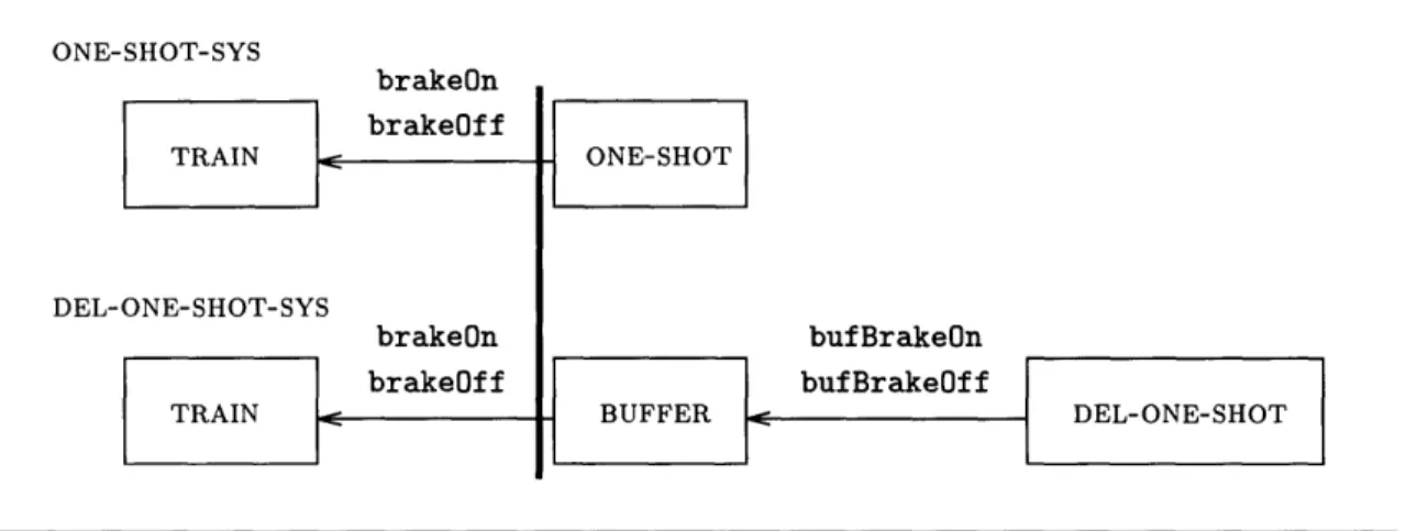
In the deceleration problem we model a computer-controlled train moving along a track. The task of the train's controller is to slow the train within a given distance. In this chapter we consider a very simple model of the train and the controller. The train has two modes, braking and not braking. The controller can instantly effect a change in the mode of the train (relaxed in Chapters 4 and 6). The controller receives no information from the train (relaxed in Chapters 5 and 6). The braking strength of the train varies nondeterministically within known bounds. We model both the train and the controller as hybrid I/O automata. Figure 3-1 illustrates the components and their communication.

In the following sections we describe the parameters of the specification, give a hybrid I/O automaton model for the train, define correctness of a controller for this train, give an example correct controller, and prove that it is correct.

Figure 3-1 Overview of Basic Deceleration Model

Sbrake0n, brakeOff

3.1

Parameters

All the parameters of the specification are constants denoted by c with some dots above it and a subscript. Dots above the constant identify the type of the constant: position (no dots), velocity (one dot), or acceleration (two dots). The dots are a purely syntactic device used to express the type of the constant; they do not represent an operation of differentiation on some function. The subscript identifies the particular

constant. Initial values of the train's position, velocity and acceleration are cs, cs, a.

The goal of the deceleration maneuver is to slow the train to a velocity in the interval

[Cminf, Cmaxf] at position cf. When the train is not braking its acceleration is exactly

zero. When the train is braking its acceleration varies nondeterministically between

[amin, amx], both negative. The range is intended to model inherent uncertainty in

brake performance. We impose the following constraints on the parameters:

1. cs < cf 2. 6s > cmaxf _ cminf > 0 3. i~ = 0 4. Emin :5 imax < 0 5. cf -- c. > 2fEX 6. < <maf--• mn--cmax - cmin

The first three constraints are self-explanatory: initial position is before final posi-tion; initial velocity is higher than target velocity range which is positive; and initial acceleration is zero. Since braking is stronger when acceleration is more negative, notice in the fourth constraint that imin is the strongest braking strength, and amax

the weakest. The fifth constraint ensures that with the weakest possible braking there is still enough distance to reach the highest allowable speed by position cf. The right

hand side of this equation uses a familiar equation for "change in distance for change in velocity" from constant acceleration Newtonian physics. To understand the sixth constraint consider that since the controller receives no sensory information from the train, it must decide a priori how long to brake. The sixth constraint ensures that

the least amount of time the controller must brake is less than the greatest amount of time that it can brake.

3.2

The TRAIN Automaton

We model the train as a single HIOA called TRAIN which appears in Table 3.1. The notation used in the table is explained in Section 2.7. The train's physical state is modeled using three variables: x, , i. As with the constants, the dots on & and i

are a syntactic device; the fact there there is a differential relationship between the evolution of these variables is a consequence of the definition of the trajectory set for TRAIN. The train accepts commands to turn the brake on or off through discrete actions brake0n and brake0ff. It stores the state of the brake in variable b. While braking the train applies an acceleration that is nondeterministic at every point but is constrained to be an integrable function with range in the interval [amin, ima]. While

not braking the train has exactly zero acceleration. The variable now represents the current time; when using assertions to reason about the timing behavior of systems, it is convenient to have an explicit state variable which records the current time.

3.3

Properties of

TRAIN

The following two lemmas and three corollaries all relate the initial state and final states of a trajectory. They establish standard facts of mechanics which we prove here for completeness. In a treatment of a system with more complex dynamics we expect that the lemmas of this section could be replaced with similar results based on whatever methods from continuous mathematics were appropriate for the specific application. We do not claim that the dynamics of TRAIN are complex or that the mathematics used in the proofs in this section is sophisticated.

In the next two lemmas we characterize the train's behavior when not braking and when braking, respectively. Below and throughout this work, if s and s' are states and x is a variable, we often write x for s.x and x' for s'.x when s and s' are understood.

Lemma 3.3.1 Let w be a closed trajectory of TRAIN whose initial and final states

are s and s', respectively, and let A = nov' - now. If b = false then the following hold:

1. i' ==O0

Table 3.1 The TRAIN automaton.

Actions: Input: brake0n and brake0ff

Vars: Output: x

E

b, a boolean, initially false

now E R>o, initially 0 Discrete Transitions: brake0n: Eff: b := true

?

:E

[amin,

imax]

if w(O).b = true then

w.. is an integrable function with range [Cmin, Cmax] else

w.J ==0

for all t E I the following hold: w(t).b = w(0).b

w(t).now = w(0).now + t

w (t).L = w (0).k + fo w(s).2 ds

w(t).x = w(O).x + fo w(s).i ds

3. x' = x+ +A

Proof: By the definitions of ± and x in TRAIN and integration. I

Lemma 3.3.2 Let w be a closed trajectory of TRAIN whose initial and final states

are s and s', respectively, and let A = nou/ - now. If b = true then the following hold:

1. & + CminA < + i <X- + maxA

Proof: We prove only the right hand side of the two inequalities; the other side is symmetric. Let z be a trajectory of TRAIN with the domain I the same as w; and let z(t).2 = imax for all t E I and z(O).i = w(O).d and z(O).x = w(O).A. Notice that

w(t).• <_ z(t).. for all t E I. Because definite integrals preserve inequalities, we know that for all t E I, w(t).. < z(t).± and w(t).x < z(t).x. Furthermore, by integration, we know that z(t).± = w(O).x + m,,xA. This establishes the first inequality. Also by integration, we know that z(t).x = w(O).x + w(O).A + ~imaxA ' _{. This establishes the}

second inequality. M

The following corollaries further describe the train's behavior during braking. The first bounds change in time by change in velocity. The second bounds change in position by change in the square of velocity.

Corollary 3.3.3 Let w be a closed trajectory of TRAIN whose initial and final states are s and s', respectively and let A = nou] - now. If b = true then the following holds:

cmin cmax

Proof: We use Lemma 3.3.2. The steps for only one side are shown:

'L < x + imaxA by Lemma 3.3.2

i•'± E< maxA subtract

c••x < 0 assumption

ax > A division

Corollary 3.3.4 Let w be a closed trajectory of TRAIN whose initial and final states are s and s', respectively and let A = noun - now. If b = true and 0 < i' then the following holds:

(&,)22 _ (2 2 - 2

2Cmin x- 2Cmax

Proof: Again, we show only the right hand side of the inequality. Let A = no] -now.

Let z be a trajectory as in the proof of Lemma 3.3.2 and let f denote the final state of z. To make the following algebra easier to read, we let i' = f.. and u' = f.x. As usual, x = s.x, ± = s.±, x' = s'.x, and ' = s'..k

x + iA + ½!maA2

I2

(Qimax < 0)

3.4

Definition of Controller Correctness

We define a brake-controller to be a hybrid I/O automaton with no external vari-ables, no input actions, and output actions brake0n, and brake0ff. A correct brake-controller is one that when composed with TRAIN, yields a HIOA whose hybrid traces satisfy the following formal axioms:

Timeliness There exists a constant t E R 0o such that for all hybrid traces if there exists a state of the trace in which now = t, then there is a state of the trace in which x = cf.

Safety In all states of all hybrid traces the following holds: X = Cf= Cminf __ •~i < maxf.

These can be stated informally as: (Timeliness) there is a length of time after which we can be sure that the train has reached cf; and (Safety) when it gets there, it has achieved an appropriate speed. The formal definitions of hybrid traces and related concepts appear in Chapter 2. Note that in (3.4) the state where x = cf can occur during time passage, i.e. within a trajectory. For convenience we call the first property the "timeliness" property and the second property the "safety" property.

26m.

(•,)2_•2

A controller which stops time before the system reaches cf is a correct controller according to the above definition. In general, one would like to avoid such vacuous correctness results. This issue is beyond the scope of our investigation, but it is treated in some depth in [1, 4, 5]. None of the of the example controllers presented in this case study stop time.

The following theorem says that the timeliness and safety properties are preserved by the implementation relation (see Section 2.4); in other words, an implementation of a correct brake-controller is itself a correct brake-controller. This theorem is not used in this chapter but rather in Chapter 4.

Theorem 3.4.1 Let B be a correct brake-controller and let A < B. Then A is also

a correct brake-controller.

Proof: By Theorem 2.6.2, A ITRAIN < B1 TRAIN. Timeliness: Let t be the constant which satisfies the timeliness property for B. We show that it also satisfies the timeliness property for A. Let a be a trace of AlITRAIN; then a is also a trace of BIITRAIN and the property holds on a by the correctness of B. Safety: Similarly. U

3.5

Example Controller:

In this section we give an example of a correct brake-controller called ONE-SHOT.

There is a broad spectrum of correct controllers from which to choose an example -from fully deterministic controllers to highly non-deterministic controllers. A fully deterministic controller would have exactly one infinite execution (ignoring e tran-sitions). We have chosen to present a controller that is highly non-deterministic:

ONE-SHOT exhibits all the possible timings of exactly one brake0n action followed by exactly one brake0ff action which a correct controller might exhibit. In other words,

ONE-SHOT exhibits all the correct braking strategies which involve exactly one appli-cation of the brake. We can imagine controllers with more non-determinism which exhibit not only behaviors with single brake applications but also behaviors with mul-tiple brake applications. We chose ONE-SHOT _{as an example for three reasons. First,}

it is easily expressed using an MMT-specification. Second, it has enough interesting behavior that the proofs of this section illustrate non-trivial proof techniques. Third and last, in Chapter 4 we use a simulation proof to show that the composition of

a similar controller and a delay buffer is an implementation of this controller. The correctness of the delayed controller then follows from the correctness of ONE-SHOT.

First we define some convenient constants:

A 1 c. - 2c .2 Cs 2amax

Cmaxf

-

Cs

The first, A, is the longest amount of time a correct controller can wait before invoking the brake. The others, B and C, are lower and upper bounds, respectively, on the amount of time a correct controller should apply the brake if it only brakes once. These constants are used as the time bounds on the tasks of ONE-SHOT.

Table 3.2 The ONE-SHOT automaton (MMT-specification)

Actions: Output: brake0n and brakeOff

Vars: Internal: phase E {idle, braking, done}, initially idle

Discrete Transitions:

brake0n:

Pre: phase = idle Eff: phase := braking brake0ff:

Pre: phase = braking Eff: phase := done Tasks: ON = {brakeOn} : [0, A]

OFF-= {brakeOff} : [B, C]

The formal description of ONE-SHOT appears in Table 3.2. The notation used in the table, called MMT-specification, is explained in Section 2.8. The controller is

called "one-shot" because it applies the brake only once. The automaton's executions

consist of three phases idle, braking, and done. It waits between zero and A time units (idle phase), then it applies the brake for at least B and at most C time units (braking phase), and then removes the brake (donephase). The ON task governs

Figure 3-2 Example Execution of ONE-SHOT-SYS 6S -Cmaxf Cminf-I I Cs _Cf

the transitions from idle to braking and the OFF task governs the transitions from braking to done.

3.6

Correctness

of

ONE-SHOT

In this section we prove the correctness of the ONE-SHOT controller. Recall that the composition of TRAIN and ONE-SHOT is called ONE-SHOT-SYS. We will present lem-mas and corollaries that establish the timeliness and safety properties for the hybrid executions of ONE-SHOT-SYS. Before giving the proof, we provide some motivation and an overview.

Figure 3-2 depicts a possible execution of ONE-SHOT-SYS. The vertical axis is velocity and the horizontal axis is position. Since the vehicle is always moving forward, the graph can be read as if time progresses from left to right. The solid line represents the actual behavior of the train in this example execution. The initial flat segment corresponds to the idle phase; the downward curve, the braking phase; and the final flat segment, the done phase. The shape of the downward curve in this execution is meant to reflect a constant deceleration, but this is the exception rather than the rule. The train's deceleration can vary nondeterministically during braking as long as it remains integrable. As achieved deceleration varies between imin and imax the curve becomes more or less steep, respectively.

The dotted lines represent upper and lower bounds that we will prove. The lower 1