Application of stochastic approximation methods to system optimization

DOCUMENT ROOM 36-412

,-

APPLICATION OF STOCHASTIC APPROXIMATION METHODS

TO SYSTEM OPTIMIZATION

DAVID J. SAKRISON

TECH N ICAL REPORT 391

JULY 10, 1962

..

MASSACHUSETTS INSTITUTE OF TECHNOLOGY

RESEARCH LABORATORY OF ELECTRONICS

CAMBRIDGE, MASSACHUSETTS

-Jtv-

The Research Laboratory of Electronics is an interdepartmental laboratory in which faculty members and graduate students from numerous academic departments conduct research.

The research reported in this document was made possible in part by support extended the Massachusetts Institute of Technology, Research Laboratory of Electronics, jointly by the U.S. Army (Signal Corps), the U.S. Navy (Office of Naval Research), and the U.S. Air Force (Office of Scientific Research) under Signal Corps Contract DA 36-039-sc-78108, Department of the Army Task 3-99-20-001 and Project 3-99-00-000; and in part by Signal Corps Contract DA-SIG-36-039-61-G14.

Reproduction in whole or in part is permitted for any purpose of the United States Government.

MASSACHUSETTS INSTITUTE OF TECHNOLOGY RESEARCH LABORATORY OF ELECTRONICS

Technical Report 391 July 10, 1962

APPLICATION OF STOCHASTIC APPROXIMATION METHODS TO SYSTEM OPTIMIZATION

David J. Sakrison

This report is based on a thesis submitted to the Department of Electrical Engineering, M. I. T., May 13, 1961, in partial fulfill-ment of the requirefulfill-ments for the degree of Doctor of Science.

(Revised manuscript received February 28, 1962)

Abstract

This report is concerned with systems whose form is fixed (either by physical lim-itations or by the choice of the system designer), but which contain a number of variable parameters. The system input, v(t), is a sample function from a stationary ergodic random process: corresponding to v(t) there is another ergodic random process, d(t), which represents the desired output for the system. The problem of interest is how to find the setting of the variable parameters which causes the actual system output, q(t), to resemble most closely (in some desired sense) the desired output, d(t).

An iterative method of solution is the approach considered here. That is, a sequence of parameter settings is generated by selecting an initial setting and then alternately observing the system performance and altering the parameter setting. For such an approach to be useful, it must be possible to show a priori that this sequence of param-eter settings converges in some meaningful sense to the setting that optimizes the sys-tem performance. We consider a particular iterative adjustment procedure and prove that, for certain forms of systems and under certain reasonable conditions on the ran-dom processes, the sequence of parameter settings generated by the adjustment proce-dure does converge to the optimum setting in the mean-square sense.

The reason for considering an iterative adjustment approach is twofold.

(i) It allows one to take as the criterion of system performance the performance function EW(dt-qt)). The error weighting function, W, is required to be convex; aside from this, it can be chosen to express the purpose of the application. This is in contrast with the usual analytic approach, which requires that W be the square of its argument.

(ii) No prior knowledge or measurement of the statistics of the random processes is required; the data are used directly.

The iterative method used here is essentially a gradient-seeking method; therefore we shall require that the performance function have a unique local minimum. This is the reason for requiring the weighting function on the error to be convex. It also places the principle restriction on the forms of systems to which the method is applicable.

TABLE OF CONTENTS

I. THE ITERATIVE APPROACH TO SYSTEM OPTIMIZATION 1

1. 1 Introduction and Statement of the Problem 1

1.2 The Iterative Adjustment Procedure 3

II. STOCHASTIC APPROXIMATION METHODS 6

2. 1 General Background 6

2.2 A Stochastic Approximation Theorem 7

2. 3 Selection of the Parameters of the Adjustment Procedure 9

III. THE DESIGN OF PHYSICAL SYSTEMS 11

3. 1 Optimization of a Nonlinear Filter 11

3. 2 Nonlinear Compensator Followed by a Fixed Linear System 19

3. 3 Bose Filter Followed by a Nonlinear No-Memory Transducer 26

3.4 The Error Criterion W(e) = I e 28

3. 5 Convexity of the Error Weighting Function and Uniqueness

of the Minimum of M(E) 30

IV. APPLICATIONS AND EXTENSIONS 31

4. 1 A More General Performance Criterion 31

4. 2 Design of a Filter when a Second Independent Channel

Is Available 32

4. 3 Compensation of a Feedback System Containing a Fixed

Linear Element 33

4.4 Simple Example - a Single Gain Setting 35

4. 5 Minimization of a Finite Time-Average Regression Function 39

4. 6 Situations in which M(x) Possesses More than One Local

Minimum 42

V. COMPUTER STUDIES AND EXAMPLES 43

5. 1 Design of a Simple Predictor 43

5. 2 Design of a Nonlinear No-Memory Filter 43

5. 3 Example: Use of the Performance Function M(x) = E{Wl[dt-q

t]Wz[dt}55

VI. SUMMARY 58 Appendix 59 Acknowledgment 73 References 74 iii 1-

I. THE ITERATIVE APPROACH TO SYSTEM OPTIMIZATION

1. 1 INTRODUCTION AND STATEMENT OF THE PROBLEM

This work is concerned with the design of systems that are optimum in a statistical sense. One has an input random process v(t) and a desired output random process d(t). In this report we shall consider only signals v(t) and d(t) which are the outputs of stationary ergodic sources. The problem then is to design a realizable system that operates on v(t) to produce an output q(t). The performance of this system is then measured by how closely (in some desired sense) the random variable qt resembles the random variable dt over the ensemble of situations encountered by the system. An example is the usual filter problem, in which v(t) = s(t) + n(t) represents a signal cor-rupted by additive noise; d(t) is then equal to the original signal, s(t). A second example is a situation in which we are given some fixed system (such as a loud-speaker or receiver circuit) that we are compelled to use. The problem then is to design a system to precede the fixed system in cascade so that, when the over-all system oper-ates on the input v(t), the output of the fixed system resembles the desired output, d(t). The usual performance criterion in such system-optimization problems is minimi-zation of the mean-square error; that is, minimiminimi-zation of

E dt-qt ] 2 .

In some applications this performance criterion is appropriate to the purpose of the application. In many applications, however, this criterion is used solely because it is the only one for which an easy analytic solution to the problem can be obtained. Here we desire to be able to deal with a more general performance criterion - minimization of the quantity

E W [ dt-qt]} (1)

in which W may be any appropriate convex weighting function on the error, d - q. In considering the system design problem we must have a convenient method for describing the system. If one is restricted to the class of linear systems, then the system may be described by its impulse response. In attempting to solve for the system that minimizes the mean-square error, an integral equation involving the impulse response is obtained; this equation, under certain conditions, can be solved

1, 2

to obtain the optimum response. In the case of the more general performance cri-terion of expression (1), no such integral equation results; in this case the impulse response is too general a description of the system to result in a problem with a tractable solution. For this reason, we might consider a fixed form for the system but leave some of the parameters free to be varied. This approach is still applicable to nonlinear systems and is, moreover, the only approach known to the author which has met with much success in the design of optimum nonlinear systems.

We shall therefore study systems that are of certain fixed forms but which contain a number of variable parameters, x, x2, ... , xk. Thus the system output, q(t), is a function of these parameters; and our problem is now to minimize the regression function

M(xl,x 2,' ... Xk) = E W[ dt-qt]}

with respect to x1, x2 .... xk. Except for the case W(e) = (e)2, there is no easy ana-lytic solution to this problem. For this reason, we turn to an iterative method of solution; that is, an initial setting of the k parameters is selected; and, by alternately observing the performance for a setting and then altering the setting, a sequence of adjustments of the parameters is made.

Such an iterative procedure is of doubtful value unless one can state beforehand that this sequence of parameter settings converges in some meaningful sense to the optimum parameter setting. Thus a major portion of this work is concerned with con-ditions that will guarantee convergence in the mean-square sense to the optimum parameter setting and with the estimation of this rate of convergence. Although the iterative procedure used here requires a fair amount of computing and yields only an approximate answer, it has two important advantages: (a) rather than being restricted to the mean-square-error criterion, it is possible for us to find the parameter setting that minimizes the mean of W(e), where W may be any appropriate convex function of the error; (b) the method does not require any prior knowledge or measurement of correlation functions or other statistics, instead the data are used directly.

The iterative adjustment procedure used here is essentially a gradient-seeking procedure. At each stage of the adjustment process an attempt is made to measure the gradient of M for the present parameter setting. This parameter setting is then changed by an amount indicated by the gradient measurement. Such a method, when used by itself, is clearly useful only in situations for which M possesses a unique minimum. For, otherwise the adjustment procedure might seek out a local minimum whose value is much greater than the true minimum of M. It should be noted that a simple problem such as adjusting the time constant of a filter for minimum mean-square error may not have a unique minimum, whether or not it does depends upon the spectra of the input signal and desired output signal. Most of the work here will be concerned with systems whose forms are judiciously selected so that the resulting performance function, M, has a unique minimum. Brief mention will be given to the multiminimum problem in section 4. 6.

One may question the advantage of being able to work with any convex weighting function on the error, as opposed to being restricted to the square of the error. In particular, Sherman3 has shown for a particular class of processes that the optimum mean-square filter (or predictor) also minimizes the expected value of any symmetric monotone weighting function on the error. However, the only member of this class of processes for which we know how to design the optimum mean-square filter (the

conditional expectation operator) is the Gaussian process, and in a given practical situation it might be quite difficult to verify the fact of whether or not the process in question is Gaussian. Moreover, as the computer study discussed in section 5. 1 has brought out, the iterative method described here does not necessarily involve a greater amount of computer time than that required to find analytically the parameter setting that minimizes the mean-square error.

1. 2 THE ITERATIVE ADJUSTMENT PROCEDURE

We now describe the iterative procedure that will be used and introduce the neces-sary notation. It is inconvenient to work with the k-tuple of parameter settings [xl,X2... Xk] as k individual quantities; hence we shall consider the parameter setting as a k-dimensional vector x. The usual inner (scalar) product

k

i=l

is denoted by [x, y], and the usual k-dimensional Euclidean norm (or length) of the vector x,

1i

(xi)2

,

is denoted by Ixl. A unit setting of the parameter xi and zero setting of the other

k - 1 parameters will be represented by the unit vector ei, i = 1, 2, . . ., k. In terms of this notation, the problem is to find the vector (or parameter setting) that minimizes the performance or regression function.

M() = E{W[dt-q x,t]}

Here, qx(t) is used to denote the output of the system with the parameter setting x. The optimum parameter setting (the one that minimizes M) is denoted by Q.

The iterative procedure used here is essentially a gradient method; that is, at the nth step of the procedure we attempt to measure the direction in which M(Xn) decreases

fastest and then change the parameter setting some amount in that direction. Such a gradient procedure is useful only in situations in which M() has a unique minimum. This imposes the principal restrictions on the classes of systems and weighting functions on the error for which the method is applicable.

We first describe the iterative adjustment in terms of sampled data (or discrete time-parameter) systems. Suppose that we have completed n - 1 adjustments in the iterative procedure; then the parameters are at the setting x n. We make the 2k obser-vations Y1 Y2 ... , y2k where

n n n

3

-r+(m-1) T 1 1 r Y =YW (t)idt-q (t)_n n x +ce m ce -n n I t=r (tn r+(2m-1) T 2 _ 1 W(t)-qx (t n x -c e _{n n-l} m

_qxn-cne1

_n t=,.+mT 'r+2kmT 2k _ 1 Yn Y Wd(t)x -xn-Cnek m W (t)n qxnck ) t=,+(2k-1) mT -k

The symbol 7 denotes the time at which the nt h iteration is started; T denotes the interval between sample times; and m denotes the number of samples used for a

.th

single observation. We form the k-dimensional vector Y whose t component is -n

2i-1 2i = y k.

Y Y = Y Y i = 1 2. k.

n n x + e x -c e. ' '

-n n-1 -n n-1

This vector Yn is a random variable, in that different intervals of data (or different sample functions) will result in different values for the observations Y , i = 1, 2, .. ., 2k.

n

Consider, however, the quantity obtained by taking the ensemble average of - Yn over

I n

the data used for the observations Yn, i = 1, 2, ... , 2k (here the quantity xn is a fixed parameter). This would also be the quantity obtained if m, the number of data samples used for each observation, was allowed to become infinite. This average, which will be denoted by Mc (n), is a difference approximation to the gradient of M(x) evaluated

n

at the setting xn with symmetric differences cn. The next parameter setting in the iterative procedure is, then,

a

x x -Y, (2)

-n+1 -n c -n' n

where (an} and (Cn} are sequences of positive numbers whose properties will be described later. The sense in which our procedure constitutes a gradient procedure should now be clear: Yn can be thought of as a difference approximation to the

c -n_n

gradient of M(x) which is subject to random variation.

The adjustment procedure has been described as being carried out in real time; this would be the case if the adjustment were being carried out on an operational system or analog thereof. Now, in order to determine something about the average system performance, we need to make measurements from a large number of different intervals of the pertinent data. In this respect, we need only require that different data be used for different iterations. Thus if the system was being simulated on a digital computer, and the observations were being made with the use of a record of

data stored in the computer, the same portion of data could be used for all 2k obser-vations needed for one iteration; the record of data would then be advanced some

amount s before making the observations for the next adjustment in the sequence. In the case of continuous time-parameter signals and systems the 2k observations used for each adjustment are made by replacing the finite sums witn finite integrals. That is, assuming that the nt h adjustment again starts at time t = T, the 2k observations

are 7+T in which _TtT n n-l 2k -1 n nek +(2k-1) Tt < 2kT

In this case, again, some time interval s is allowed to elapse before making the observations for the next adjustment.

The reader may wonder if it would not be more expedient to use only k + 1 obser-vations for the estimate of the gradient, rather than to use 2k obserobser-vations to obtain a symmetric estimate. Sacks,4 whose work is mentioned in Section II, considers this point and shows that, in the general case, when the performance function M() is not

symmetric about its minimum, the estimate of the rate of convergence is actually made faster by using 2k observations.

In Section II we are concerned with the mathematical conditions necessary for the convergence of the adjustment procedure described above. In Section III these con-ditions are related to physical requirements for two specific forms of systems. In Section IV we present some applications, and in Section V discuss several examples and computer studies.

II. STOCHASTIC APPROXIMATION METHODS

2. 1 GENERAL BACKGROUND

The iterative procedure described in Section I is an example of a Stochastic Approximation Method. In particular, it is a multidimensional extension of the Kiefer-Wolfowitz method for locating the minimum of a one-dimensional regression function by making a sequence of observations of the random variable. Assuming certain regularity properties on the function M(x) and that the variances of the Y_n were finite, Kiefer and Wolfowitz5 proved convergence in probability of the sequence {xn-0} to zero for suitable choice of the sequences an} and {Cn}. Blum6 showed con-vergence with probability 1 for a multidimensional case. Sacks made extensive esti-mates of the rates of convergence for both the single and multidimensional cases under a variety of restrictions on the function M(.). Dupac7 made estimates of the rate of convergence for the one-dimensional case for a variety of choices of the sequences {an} and {Cn}.

Now let us consider the distribution of x n. We note that our basic sample space (or probability space) is the space of sequences of data {v(t)} and {d(t)}, t = 1, 2, ... , T, where T is the time at which the (n-l)th iteration is completed. The parameter setting xn depends upon both x1 and on the data used, hence the probability distribution for xn depends on x1. Thus in referring to xn we are actually speaking of a family of random variables, xn(x1), indexed by the initial parameter setting x1. Now, in arriving at the quantity

M = E {Yn} (3)

Mc (Xn) c

n n

the averaging is over all pairs of sample sequences v(t) and d(t). In the expression

_F(l,Xn) = E {Yn _Xn(Xl)} (4)

the averaging is only over those pairs of sample sequences that could have caused a transition from the parameter setting x1 to the parameter setting xn. In both cases, x itself is considered as a parameter, although in the second case our conditioning

4-7

depends on x1 and x n. In the work cited above, it was assumed that

Mc( n) C= 1F( X1'Xn) (5)

n n

This will hold true, for example, when the data used for one iteration are independent of the data used for each preceding iteration. The condition expressed by Eq. 5 is too

restrictive for the problem at hand; hence we present an extension of the work of V

Dupac.

2. 2 A STOCHASTIC APPROXIMATION THEOREM

We state some assumptions on the regression function M() and on the processes Yn and xn(x1) which allow us to make statements about how the sequence

{([_n-0

1 2) con-verges to zero in the mean. In Section III we shall translate the assumptions made here into conditions on the physical design procedure; the implication of the statements made here to the convergence of the physical design procedure will then be more or less obvious.

We make the following assumptions:

(a) M(x) is decreasing in the direction - x for all x of interest.

(b) The gradient of M evaluated at x [written (grad M)(x)] is suitably bounded in magnitude.

We must also make some assumption on how rapidly the term

Fn(Xl) = I E{[Xn e Yn(Xn)CnMc (Xn ) ]}[ (6)

n

approaches zero; that is, roughly, how much the process depends on the information about its past that is contained in xn - . We shall assume that

an/2

Fn ) < S1 Cn/2 S1 < (7)

in which S1 is independent of x, the initial parameter setting. We shall show in Section III that inequality (7) corresponds to an extremely broad class of physical processes.

In order to make these ideas precise we make the following assumptions: (i) E{1Ynl 12 X l) < 11 E{Y nn(X)}1 2 + S S < ;

(ii) (a) K x 0 12 [ (grad M)( ),+(x-0) ],

(b) 1I (grad M)(x) || Kll x-0 1 K1 > Ko > 0;

an/2 (iii) (a) Fn(_l) = E{[xn -O YnLn) CnMc )] SC

n n/2

(b)

EIIEYE

n(Xl)}

n

1

2

_-cn

_{Mc nXn)}

_{12}J 1}

n

in which S1 < o, S2 < , and S1 and S2 are independent of x for allxl E X (see (v)). (iv) {an) and {cn} are sequences of positive numbers satisfying

o00 00 00 2 0 0 a

a 2

E (an) ' E a an~n s S (a a n/2

a n=co,

Z

(an)2 <C ~ ac <00,

(

< , and n an < 00

n=n = 1=1 n n1 n=1 n/2

7

in which an/2 and cn/2 are suitably interpolated for n odd.

(v) x is constrained to a bounded, closed, convex set X, but is free to be varied inside X. (A set X is convex ifx 1 e X, x2 e X implies ax l + (-a) x2 X for 0 < a `< 1.) Assumptions (i), (ii), and (iii) need hold only forx e X. It is assumed that X is chosen

sufficiently large that 0 X.

We now make the following statements.

STATEMENT 1: Assumptions (i)-(v) imply the convergence of 11xn(x)-.0 to zero in the mean-square sense for all x1 X. That is,

lim Ex (xl)-01 2} O for all xI X. n-Boo

We now set an = a/n cn c/nY, and thus to satisfy assumption (iv) we require 3/4 <a < 1, 1 - a <y < a - 1/2. We also require a > 1/Ko if a = 1.

STATEMENT 2: Assumptions (i)-(v) and the choice a = 1, = 1/4 imply that for all x1 E X

E fXn(Xl) 0 12) = 0(1/n1 / 2 )

(f(n) = 0(g(n)) means lim (f(n)[/[g(n)) < +oo n-Boo

Furthermore, this choice is optimum in the sense that no other choice guarantees faster convergence for all Y(x) satisfying assumptions (i)-(v), that is, for a 1, y 1/4 there exists a Y(x) satisfying (i)-(v) so that

E|xn(x)- 11' = (1/nl /2 ) for some E > 0. STATEMENT 3: Under the added restriction

a3 M X)

< Q < 0o i = 1, 2, .. , k and x E X, axi

the choice a = 1, y = 1/6 implies that for all xl E X

E lxn(x1 )- II2 = 0(1/n / 3),

and this choice is again optimum in the sense of Statement 2.

The proofs of Statements 1-3, which are given in Appendix A, follow the same V

general lines as those of Dupac. We only comment on the intuitive reasons for the different assumptions. The first assumption requires that the variance (as conditioned by xn(l)) of the norm of Y must be finite. If one wishes to think of Y as a difference measurement of the gradient of M(xn) with "noise" superimposed upon it, then assumption (i) is a restriction that the "average power of the noise" be finite. Clearly, some such restriction is necessary. Assumption (ii-a) provides that the slope of M(x)

in the direction of the optimum parameter setting never be too small; assumption (ii-b) requires that this slope never be too large in any direction. The first condition pre-vents the adjustment process from "sticking," while the second prohibits sustained oscillations of the adjustment. In considering assumption (iii), note that

n-1 a. J

n(X-l) = Yj() j +x-1 (8)

j=l j

and thus assumption (iii) is a restriction on how the process Yn may depend on its past. There is little that can be said intuitively concerning assumption (iv), except that we require

00

an

=

n=1

in order that the process be capable of reaching the optimum setting, no matter how far away from the optimum setting it may be on the nt h iteration. Concerning assumption (v), the restriction that X be bounded is not necessary at this point, but will be required when we translate assumption (iii) to conditions on the physical situation. It is neces-sary that X be convex in order that there exist a "downhill path" from all x E X to O. If 0 does not lie in X, then the process will converge to that setting in X, say 0', for which M is a minimum, provided that assumption (ii) still holds with 0 replaced by '.

2. 3 SELECTION OF THE PARAMETERS OF THE ADJUSTMENT PROCEDURE In the iterative adjustment procedure described in section 1. 2 there are several quantities that may be varied: s, the time interval that separates data used for suc-ceeding iterations; m, the number of data samples used for each measurement of Y c e; and the coefficients a and c when a a/n', cn = c/nY. The statements of

x-n n-i

the preceding section estimate the convergence of the parameter setting as

b_{bn =E} n E ([[-n(Xl)-o[2 _x )_ _{_} C 1_C 1 ₍₉₎ n

In expression (9) the rate of convergence (6, the exponent of n) is not affected by the quantities s, m, a, and c. The coefficient C does depend on these quantities, however, and a brief investigation of this dependence is in order.

In the general case there is little that can be said because there is no reasonable assumption to make concerning the dependence of the coefficient S1 upon s. For this reason, we consider the case in which the data used for each measurement of

i

Yn, i= 1 2 ... , 2k, n= 1, 2, ... are independent of the data used for all other measurements. We denote by T the time taken to make a measurement of Y , using one data sample for each of the 2k measurements Yn, i = 1 2 .... 2k. Then, from

9

expression (A-21), we have (noting that S1 = S2 = 0 for this case) 2 Fac + D a S(m) b c n Ea - 1/2 ()l1/2 1 S

in which t = nT is the time required to complete n iterations. Now if the average of m independent observations is used as a measurement of Y, i = 1, 2, ... , 2k, then

n S(m) = S/m.

If we substitute this expression for S(m) in Eq.(10) and m which minimize the coefficient of (t/T)-1/2, we find is redundant; and that the minimum is determined by

solve for the values of a, c, and that one of the three relationships

a= 1 + -1/2

2E 2E)2 2E

c4mF = DS .

(11)

(12) Of the two parameters, c and m, one may thus be fixed and the other determined by (12); the optimum value of a is always determined by (11). Since the quantities E, F, and D are unknown, the optimum values of a and c may not be determined directly. It is, however, possible to effectively estimate the values of E, F, and D during the course of the adjustment procedure and change the values of a and c to conform to the values given by Eqs. 11 and 12.8

10

(10)

and

III. THE DESIGN OF PHYSICAL SYSTEMS

3. 1 OPTIMIZATION OF A NONLINEAR FILTER

We shall now consider several system configurations whose performance can be optimized by the adjustment procedure described in Section I. The main limitation on the system configurations that we can treat is that they must yield a regression surface

or performance function, M(), which has a unique minimum satisfying assumption (ii-a). The primary result will be to establish that assumptions (i-v) of section 2. 2 are satis-fied for the given systems.

The first case that we consider is the design of a filter (or predictor or model) of the form shown in Fig. 1. The first reason for selecting this form is that it is general

in the sense that any continuous nonlinear operator whose output depends only remotely on the distant past can be approximated arbitrarily closely by the given form if a suf-ficiently large number of terms is used.9 A second reason for selecting this form is that the output of the filter depends only on the present setting of the parameters x1, x2' '... xk and not on their past history. This makes the adjustment procedure

much easier to analyze. It should be pointed out that if a good filter is already available, it may be placed in parallel with the filter of Fig. 1, and its output multiplied by a

qx (t) OD

Si(t)

= hi () V(t-r ) r = O So (t) = h(r) V(t -r) dr 0

(DISCRETE TIME PARAMETER CASE)

(CONTINUOUS TIME PARAMETER CASE)

i= I, 2, , j

.-Fig. 1. Form of the filter to be designed.

11

gain Xk+1 and added at the indicated summing point. For the parameter setting x1 = x2 = . . x. = xk = 1, the over-all filter reduces to this original filter; and hence the performance of the over-all filter must be at least as good as that of this original filter.

We desire to use the procedure described in Section I to adjust the gain coefficients xl, X2, ... , xk of the filter in Fig. 1 so that the performance function M(x) = E{W[dt-qx,t]) is minimized. Subject to the restrictions stated below, W should be chosen to be appropriate for the purpose that the filter is to accomplish. The following restrictions are sufficient to guarantee that the statements of section 2.2 apply to the adjustment procedure:

(a) v(t) and d(t) are the outputs of stationary ergodic sources and are uniformly bounded in absolute magnitude for all t with probability 1.

00

(b) I hi.(t)[ < 00; i = 12, 2 . . k. The fi(t) = fi[sl(t), s2(t), .. .s(t)] are continu-t=o

ous in sl, s2 ... , sj fori = , 2, ... k.

k )

(c) P E (x.-0) f a D x-Oi=l for x EX and D E>0.

Or, in terms of one sample function, there exists an No with the property that for N > NI _{fo 2N + 1}2Nn+ 1 E > 0, where n is the number of occurrences, -N t N, of

k

, (xi-Oi ) fi(t) >- Dx 0-e{ x e X. i=l

(d) W(e) is a polynomial in e of finite degree. (W(e) will thus possess bounded continuous derivatives.)

(e) W(e) is "strictly convex"; that is, there exists an E > 0 with the property that W[aa+(l-a)b] -< aW(a) + (-a) W(b) - Eala-bl2 for 0 a 1/2.

(f) Assumption (v) is required to hold directly; that is, our parameter adjustments are confined to a bounded, closed, convex set.

(g) Consider the random processes, d(t) and fi(t), i = 1, 2, ... , k; t may take on either discrete or continuous values. Let F1[fl(), .. ., fk(T), d(T)] be any bounded con-tinuous functional of d(r) and the fi(T), rT t. Let F2[d(), fl (r) .... fk(T)] be any bounded continuous functional on d(T) and the fi(), t + a T t + a + T, T fixed. Then we make the following requirement on the correlation between F1 and F2 for large a

iRFF2

IE{(Fl Ff 2)}I a 2 F1 F2

in which K is independent of F1 and F2. If d(t) and the fi(t) are discrete time-parameter processes, then F1 and F2 are ordinary functions instead of functionals.

t .- a -Fl[fl (r) ,', fk(),d(T)] r t Ft [f, (), ,r fk(T), d ( ,)] t+a<T < t+a+T 2- F2 a DICTION OF F2-F 2 T= t PRFnlICTION FRROR "ALLOWABLE" PREDICTION FgCpnm 2 F2

2 [I-K I LOWER BOUND ON

-F2 -a4 PREDICTION ERROR

/~~~~~/ \>4FOR LARGE a

a

PREDICTION TIME

Fig. 2. Explanation of restriction (g).

To gain an understanding of restriction (g) and appreciate its generality, the reader may wish to consult Fig. 2. The quantity F2 is obtained by some operation on the data in the interval t + a -? - t + a + T. Now let us try to predict F₂ by using some functional, F₁, on the data for T t. Note that there is a spread of a seconds between the data used for F2 and the data used for F1. Now the best (mean-square) linear pre-diction of F2 - 2, given F1, is R

1 2

RF (F1-F1) 2 2 2 1 QF1

and the mean-square error in this prediction is

13 Ua t t+a t+a+T r

Y-v-i

I I %

__ --I -fi ( fl , i = k·,

1 22 '2 2 2 F 1 F2 RF1F2 F1

Thus our requirement on R F F is only a stipulation that the data d(t) and fi(t), i = 1, 2 ... k, be such that our ability to predict some function of the future data diminish as the prediction time becomes large; in particular, the error must approach its asymptotic value at a rate of 1/a4 as a becomes large. Note that if d(7) and the fi(T), t + a - z 7 t + a + , are statistically independent of d() and the f.(7), rT t for

1 1

> a , then R - for a > a

o F1F 2 o

Restrictions (a)-(c) provide no serious limitation on our physical situation. Restriction (a) will surely be satisfied, since the output of any physical source is always uniformly bounded. Restriction (b) requires only that the memory elements h1, h2, ... h. be stable and that the fi be continuous, as all physical transducers are. Restriction (c) only requires that all the h and all the f differ from one another in the

prescribed sense. An alternate statement of restriction (c) could be that the fi are all linearly independent random variables. A proof of this statement is given in Appendix A. 5. Restrictions (a) through (c) are expressed in terms of the discrete time-parameter case; the alternate statement of these restrictions for the continuous case is obvious.

Restriction (d) is no real restriction in addition to (e), since any convex function is continuous and hence may be approximated arbitrarily closely of the finite domain of W by a polynomial. Note that restriction (e) is stronger than the usual definition of strict

convexity; it in fact requires the polynomial W to contain a non-zero quadratic term. As discussed in Appendix A. 5, this may be relaxed to the usual concept of strict con-vexity by slightly strengthening restriction (c). Restriction (e) imposes the only serious limitation on our method. Restriction (f) imposes no serious limitation on the allowable parameter settings. Restriction (g) is quite liberal for a nonperiodic random process. It should be added that the rate in restriction (g) could be reduced from (1/7 2) to (1/7 +), > 0, although this would affect the estimate of the rate of convergence as given by Statements 2 and 3. For periodic processes restriction (g) will not, in general, be satisfied. This checks with our intuition; if the frequency of the process were in

synchronism with the adjustment procedure, we would expect trouble.

We shall now prove that restrictions (a)-(g) are sufficient to guarantee that the assumptions of Section II are satisfied. The proofs are carried through mainly for the sampled-data case, with comments made at the end to indicate the extension to the continuous time-parameter case.

To show that assumptions (i) and (ii) follow from restrictions (a)-(e), we use the ergodicity of the sources to write

N k

M(_ = EW[dt-qt] =im 2Nl 1 W (t) - (13)

14

Assumption (i) now follows immediately from restriction (a) on the uniform boundedness of the sources, and from restriction (b) on the form of the filter.

To show that the upper inequality in assumption (ii) is satisfied, we use a Taylor's expansion about x = 0 to write

aM(x) a M(x)

0+ (xi-O .0 = + XT.e. (14)

~~a~~~

ax

3J i=l

where 0 < . < 1 for an arbitrary j, with j = 1, 2, ... k. Thus, the upper inequality in

1

assumption (ii) follows with

a 2M |x

kl = k sup ax ax

i,j=, 2 .... k 1 3 X X

a 2M(x)

if all the 8ax. x. i,

j

= 1, 2, ... k are bounded for all x X. To show this, we consider N k SN( = 2N + 1 d(t) - E ifi M t=-N i=l and

N

k

S 2N + 1 W" d(t) xifi(t) fi(t) f(t) t=-N i=l

The continuity of W" and the uniform boundedness of the f(t), i = 1, 2, ... k and d(t) imply the equicontinuity of SX for x E X. The Arzela-Ascoli theorem then guaran-tees the existence of a uniformly convergent subsequence Nm , and for this subsequence

2 a2

. lim S lim SN () li lim S ( (15)

ax.

8_{x N ax.ax.N}

= N

1 m-*oo m m -0 1 m m-00 m

for all x E X. However, by our assumption of ergodic sources, lim SN(x) is unique

N-0 °

with probability 1, and hence

82 1 N

r

xix M( ) = lim 2N + W d(t) xifi(t)j fi(t) f(t) (16)

t=-N i=l

with probability 1 for all x E X. But the right-hand side of Eq. 18 is bounded by restrictions (a) and (d), and we have established the upper inequality in assumption (ii).

We now turn to the lower inequality in assumption (ii). Using Eq. 13, restrictions (c), (e), and the convexity of X, we have

15

-. _ 2_ ,,,, v9

M[ (1-ac)+ao0] (1-a) M(x) + aM(O) - EDEalx-O11' for 0 a < 1/2 (17) or

M[x+a(0-x)] - M(x) M(x) - M(0) 2

MX )- - - + ¢D2EI(x_-_OJ[D 2E(x-O[ a 2EElx-Oli [D for 0 a 1/2.

(18)

The right-hand side of Eq. 18 is independent of a; hence, taking the limit of the left-hand side as a approaches zero, we have

f-+((1) 2

(grad M)(x), ] eD2 Ex- j (19)

as desired.

If we desire to use the results of Statement 3, we need only use in addition the fact that W'" (e) is continuous for all values of the argument which occur under restrictions

(a) and (b), and the assumption that x X. The boundedness of a3 M(x)

i= 1,2,... k 3

ax.

i

under this added restriction is shown in the same manner as was the boundedness of a2M(x)

ax. ax. 1

In the continuous time-parameter case the performance or regression function

00

M(X) = lim _ f w[ d(t)-q (t)] dt can be written

T-co -o

M() = li 2N + 1 N m+l)T W[d(t)-q (t)] dt

00

~m=-N

mT

and these proofs are directly applicable to this case.

Assumption (iii-b) follows immediately from restrictions (a) and (b).

We shall now show that restrictions (a), (f) and (g) imply assumption (iii-a). We wish to bound

Fn(Xl)- Ex 0 Y n(X)CnMcnf x (20)

FPx₁ ) · I~i L~ -~," (20)

The inner product in (20) consists of k terms. Consider the magnitude of the ith such term

F.i, n E(Xi, n-0 IY. n(X )-C M. _{n n l,} (x ) . (21)

If we can show that each such term satisfies our bound, then Fn() must also. Now, 2i- 1

Y. consists of the difference between a measurement, Y , with x = x + c e. and

1, n-1

another measurement, Yn', with x -c e. We shall consider only the difference

a2i, w -n x=i

between y2i and M In+cni), and neglect the terms resulting from the c's (which will be smaller than the terms considered). We also assume that only one data sample is used for the measurement. These assumptions will not restrict the generality of the proof, but will help to simplify the cumbersome notation required. We thus wish to

estimate

F.' = E in -) i

L

d

x. X, n -

EWdn

L L -1, n-8i n n

C · i1

1,

i=l

in which the expectation inside the brackets is taken with xn as a parameter. restriction (d), (22) Now, by k W d -

L

x. f. W dn xi, nfi, n i=l N j=0

j

(

k

m

B jmd n - Xi, nfi. n m=O i=1 N j /

-=

Bjm dn j=O m=O k N-j z i=l m n xi, nfi, n) N There are a total of

j=O terms in F! n; a typical

1,n

E (k)m terms in this sum, and hence m=O one of these is k m. i, n m i n j=)1 j, n ,k 1 J k N a total of

L

j=o km 0 M=O (dn) N-m-j (f ,n) - (dn) () N- (f J j=1 j=l(24) (24) in which mj = m. Thus if we can show that this term is bounded, we shall have

j=1

shown that Fi n is bounded. We consider only the first of the two terms in Fin (the

1, n 1,

Xi n term); the second (the 0i term) can be treated in a similar manner. For this first term we have Fim 1 C M Xd n )

I

j --1 j - dN-m (25) J=! 3 For simplicity, let n denote

(dn)-m

j-- (f

j

n)

- dn)Nm

1

(f Also, recall that

17

(23)

__

-a in which -- Y.

C 1, 0

Thus (25) can be rewritten as k = Cm i, n - Xj, n) 3=1 m. Pn n-l n-1 C m

3

qj=° q2=O n-1 a a q q 2

Z

c c qm+l= q q₂ n-1 q ql = ° q2 n-1 m, 1 + i, n q2=0 +... + m+1 terms n+1

Cm

qm+l=° *1 -I =O0 q2-1

Z

*1 a q l qro+l= ql q2 q2

Z -

..

Z

1=0 q3=0 q+l qm+1- qm+1 - 1 a qrn+l C,, qml a a C c ql qm+l

l

3

I

]

a a

S

q q m+l a = q1 qm+l = m+1 terms n- a Cm. c ql=O n-1 + Cm

S

q2=0 +... + n-1

CM

Z

qm.+l= 1ql ql a q2 c I 2 1 k m. Y. 1 Cx +)JP i = 1 2 m. Yi2, q2 j ( , q2+1 a qm+l c 0 qm+l Y. -1 m+l' qm+l j= 1 j, qm+l + 1

Now, recalling that a

O y

c 1, 0 = xi, o we see that the zeroth term in each of the m+1 sums

18 n- a q Xi, n= C- Yiq q-0 q xi, 1' r, 1 F, n 1, n or a qm+l c L m+l J (26) I a Ylq ... Yi q Pn i1'91 m+l' m+ I Pn Pn Y il , .YiP I'gl m+1' m+1

is of the form

1 1

k m. k m.

i _Xil~l j r1 (xj, 1) Pn Xi _{1 j= l}X1 (xj, 1) J Pn

for all xl E X. Thus by using restriction (g), each of the m+l sums in (26) can be bounded in magnitude by n-l a.

=K

12 1 =1 c(n-j 2 j=l (n-j) for all x1 e X in which 0 -K 1 - Ysup jIsup Cm m .

But for any sequence aj/cj for which aj/cj (n-) to some point i and monotonically increasing from

cn = c/n_n 7), it is shown in Appendix A that the sum, an/2 (in which Cn/2 finite number of K2 2 n/2

is suitably interpolated for n odd).

is monotonically decreasing from 1 i to n-1 (which includes an= a/n a,

n 1' can be bounded by K2 (n/2I

Cn/2 Thus we have split Fn(l) into a terms and shown that each term could be bounded in magnitude by

all x _1le X K2 < and, since

1jl -<zI

1

we have Fn( 1) < K3 n/2 Cn/2 all x1 X as desired.

Note that the derivation above remains valid whether (d n)N- and (fi n ) m' i = 1, 2, . . ., k, represent discrete time samples or finite time integrals of continuous processes, as they would when d(t) and v(t) are continuous time-parameter processes.

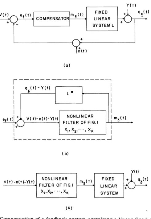
3.2 NONLINEAR COMPENSATOR FOLLOWED BY A FIXED LINEAR SYSTEM We now consider the more general situation shown in Fig. 3. We are given some fixed linear system whose impulse response is h(T). By constraint of the design

19

(27)

K3 < (28)

e(t)

qx(t) = E h(r) m (t-r) (DISCRETE TIME PARAMETER CASE)

r =O O

qx(t) = h(r) x(t-T)dT (CONTINUOUS TIME PARAMETER CASE)

Fig. 3. Cascade compensation of a fixed linear system.

problem, this system (which may represent a loud-speaker or circuit or other device over which the designer has no control) must terminate the over-all system. We wish to precede this fixed linear system with a nonlinear compensator in order that the over-all cascade system be optimum. The nonlinear compensator to be used will be of the form of the filter of Fig. 1, and restrictions (a)-(g) of section 3. 1 will again be imposed. We now wish to establish the validity of assumptions (i)-(iii) of Section II.

Assumptions (i), (ii-b) and (iii-b) follow directly from replacing the functions fi(t), i = 1, 2, ... , k by the functions

00

gi(t) Z h(r) f(t-T) i = 1, 2, . . k, (29)

'=0

oO

provided that I h(j)

f

< o. Assumption (ii-a) follows if we replace the functions fi(t) j=O

in restriction (c) by the functions gi(t), i = 1, 2, .... k.

Establishing assumption (iii-a') is another matter, however. Since the linear system possesses memory, the output of the over-all system, q (t), will, in general, depend not only on the present value of the parameter setting but also on the past history of the parameter settings. This problem would not arise if the linear system had -a finite memory of T seconds, and T seconds were allowed to elapse between the end of one observation, Y_n n, and the beginning of the next observation, yin +l. _n This, however, is too restrictive a condition to impose on most systems.

Let us consider the source of the difficulty for a single parameter. We need to measure the quantity

M(X-Cn) {W[ dt-h o(X ) ft-hn-n) n-c ft-h n) ft 2-h3(xn-c n ) ft-3-' ] } but we are observing

20

Yx -c = W[d(t)-h(x n - c n)f(t)-h 1 (xn+cn) f(t- 1) n n

-h 2(xnl-cni)f(t-2)-h3(Xn l+c n _ )f(t-3)- ..

Now Ixn- 1 < Kan/cn approaches zero fast enough that these terms can be taken

care of by requiring that the impulse response fall off sufficiently fast. The difference introduced by having xn + cn in place of xn - cn, however, only approaches zero as fast as cn; and hence will prohibit us from proving convergence as before. These trouble-some terms may be eliminated by using the adjustment scheme shown in Fig. 4 for the two-parameter case. The systems h () are used to simulate h(7). They need to

resemble h(T), in the sense that

EtT t)

=gi,

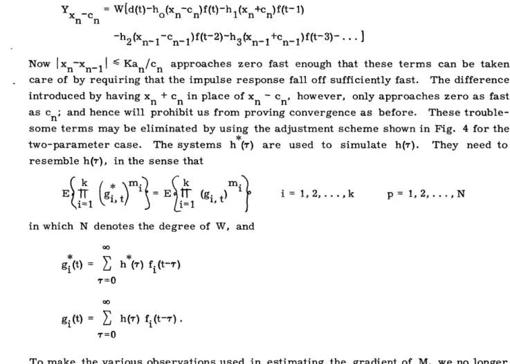
Et (gi, t) 1, 2, . . .,k = 1,2,.., in which N denotes the degree of W, and

00 gi(t) = h (r) fi(t-T) T=0 00 gi(t)= h (T) fi(t-T). T=0

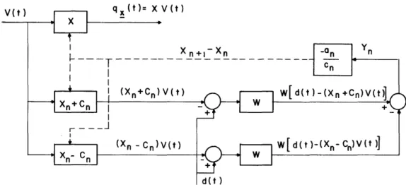
To make the various observations used in estimating the gradient of M, we no longer directly perturb the coefficients x1 and x2, but rather vary the gains of the amplifiers shown as 0 and c n. For example, to measure Yx +c e we set the top amplifier at

+c and the bottom one at 0. n n1

n

As mentioned above, we need to make a restriction on the rate at which the impulse response h(T) falls off. In particular, we require

I

Fig. 4. Arrangement for adjusting system parameters.

21

I_

__

K < oo. > 1.

We now establish assumption (iii-a). We shall restrict ourselves to considering sequences of the form

a a/n a c = c/n

n n

For notational convenience, we consider only the one-dimensional case (= x, a single parameter); the method used holds true for the multidimensional case. We assume, for simplicity, that only one sample is used in making the measurement Y1 and the

n

measurement Y2. Of the two terms (xn+0)[ Y-M(xn+ cn)] and (Xn+0)[ Yn-M(xn-cn) we consider only the first. We shall also ignore the terms that are due to cn as being smaller than the terms considered. These assumptions do not restrict the generality of our proof, but serve to simplify the details. We thus wish to bound

n (XnO)LW[d n E hx jfn- E WX

L_ (x, j=0

n-i

(x-0)

W n-

h.x -Jfn-f -

E

W

in which xn, Xn_ ... , xi appear as parameters in the expectation shown inside the brackets. We consider the first term on the right-hand side of inequality (30), first. Let n-1 n-1 a=dn hjxnfn.j and b = dn E hjxnjfnj j=o j=o then n-1

a-bl -<

f

sup E I hjlX Xn-Xn-jsup' (31)

j=0

Now, by virtue of the fact that signals f and d are bounded, Yn is bounded in magnitude; thus

n-1 n-l

a. a.

Xn -Xn-j sup Ylsup I E c. C.

i=n-j i=n-j

with K2 < oo, and K2 independent of x1.

22 i · I I (30) (h) I h(,r) -< I-r

Thus for an/cn = a/c' l/n a -l,

Xn-xn-jIsup _sup K2 e _{n-j- 1} I da _6c c En-l) (n-j-1) (32)

in which 6 = - (a-y). Using restriction (h) and inequality (32), we show in Appendix A. 4 that we can give the following bound for the sum appearing in (31):

n-1 "2 d I--<- nl) --- K 1 2 Xn n-jsup 3 -j=O n Thus (31) becomes i a i sup 3 - K3 < , independent of x (33)

Now, W is a polynomial whose argument takes on a bounded range, hence over this range

dW L < oo

de

_sup

and thus

IW(a)-W(b) LIa-b! I LK' 1 (34)

sup sup 3

na-with LK < and LK' independent of x. Thus the first term of (30) is bounded by

3 K 3 independent of 1,

Ix-o sup LK'3 /na = K' 1/nt with K3 < , and K3 independent of xl.

We turn now to the problem of obtaining a bound for the second term in (30). This can be expressed as T = (Xn-0) Wdn- hjxn-jfn -E _ W j=0 N m m \q f Nm qli (5x 0)E E bm(d n -m | hj Xn jfn -E (d.x .f (36) m=O q=O j=0 =

in which the expectation inside the brackets is taken with xn, xn-1 . , x1 considered as parameters. Now, Eq. 36 contains N(N+1) terms, N(N+) multiplied by x and NN

2 n 2

multiplied by 0. We pick the (N+l)Nth term, Tm , of these first N(N+I) terms and derive

2 2

a bound for its magnitude. The other terms can be bounded in the same fashion.

23

_I _ _ _ _

m - E T n - 1 j=0 h .x I J n-J n-J (d )N-mnd, n-1

z

j=0 mh h x -f ) J n-J n-j n-1 n-1 = bm Z " h. ... hm j1'0~~~~~~ .f -(n Xn x . (d)N-m f nn-J n-J m n -J1 * fn-Jm_-(ci (dn m N- fn f ... n-J 1

As in section 3. 1, we can split the multiple summation up into m terms, the first of which is n-1 ITm 1 - bmmJ C ii =0 j 0

z ..

1

j2= hj ... h j =01 jm Jm=0 xnx ... nj -m f .... f n n-j Xf~f~~*. Xl~[m jnJ

'~

d~n)j 1 n-J m -n-1 bmm 1c)N-r **flm (dn)N-m f ... f -m| ii j Z

Z

_, h. l ... h. J - 1 im JrV 2 JmU n n- 1 .. xn_J (dn)Nm n-j n-jM

~~

n-JI n-i - (dn)N-m_fn-J fn-(37) Note that in this sum , )- i k, k = 2, ... , m; for convenience, we shall denote the term

(dN-m _{f .... f}

n-J 1 n-Jm

Note that Pn n-j depends only on data v(T), d(T), for n-jl T n. Now 1,n-

let the summand in (37) be denoted by

A = Xnj X..jm n, n-jl

Now note that since jk jl k = 2, 3 .... 3. m, we can express xn, Xnj _·

_~~~~~~~-

_{2 ,} ... _, xn-j_{n Jm}

n-jk = Xn-jl +(x n-jXn-j n-J k nJ x _Xn = x n _Xn-Jl + (Xn-x nj ) n n-J1/ 24 by pn, n-j1 - (d )N-mf n-j ... fn-Jn- '38) as _ _ _ . -: _n: k = 2, 3,...,m

Substituting these expressions in (38) yields A as the sum of 2m terms; one of these is

n-j)m+ PnJ n-j 1 (39)

and the other 2m-1 are of the form

(40) tXn-j m+l n-l-xn-jl... n-i -Xn-JPn, n-Jl

in which i, i2 ... is, denote any distinct collection of s of By the reasoning used in section 3. 1 and restriction (g), the term given by (39) is bounded by

an- 1 2 K' 2 4c n-j 1 2 1 or K 1 (n-j 1)

with K4 < o, and K4 independent of x1. Next expression (40). Let

B = sup Ixl-X 2I xleX

x2eX

* = IPn, n-j sup

the indices 0, ij2 ji3 . .. m' it is possible to show that

a

n a 1

for =

-c _n c a--y_n (41)

consider the terms of the form given by

Y =lYnsup_{n sup} Then, since n-l a

q *

I

n n-j 1 qn-jjl q it follows that

IXn-Xn-Jlj

~J

n~J

1

k = 2, 3,..., m

and thus we can bound each of the 2-1 terms of the form given by (40) by

n- a

q q=n-jl q

for all x1 e X.

Now for aq/cq = a/c 1/q a - ', we have shown that

q q n-l a q c 6[(n-1) -(n-l-j ] qn jc -6 1) q=n-j q 25 --- I

in which 6 = 1 - (a--y). Thus it follows that the 2 - 1 terms of (38) that are of the form (40) can be bounded by

for all x1 E X. (42)

Now comparing expressions (41) and (42), we see that each of the 2m terms making up the quantity A can be bounded in magnitude by

K6 1 [ (n-1)6-(n-j 1-) 6

K

K₆ n1 6 na-'y j =0 for all m -M S m < M for all x1 E X.

Substituting this bound in (37), we obtain

IT

m \ -<b K (ho)m+l 1 I mm 6n n-1 +bmmK62m j1=1 il j2=0 - b K (h ,m+l 1 -mm 6 ) n_nay

L

im-1 +b mK6 2m

([

hI n-1 Z Ihj-1

-

[ )6 (n-1)-(n- 1-j)6] j=l

for all x1 E X. It is shown in Appendix A. 4 that the sum in inequality (43) can be bounded by K7 1/n a - ', and thus Tm 1 K8 1/n 7' , for all x1 E X.

We have thus split Fn(x1) up into a number of terms (the total number of which depends only on the degree of W) and shown that each term can be bounded by Kg 1/na - ', for all x1 e X, and thus Fn(1) < K10 1/n a- , for all x E X, as desired.

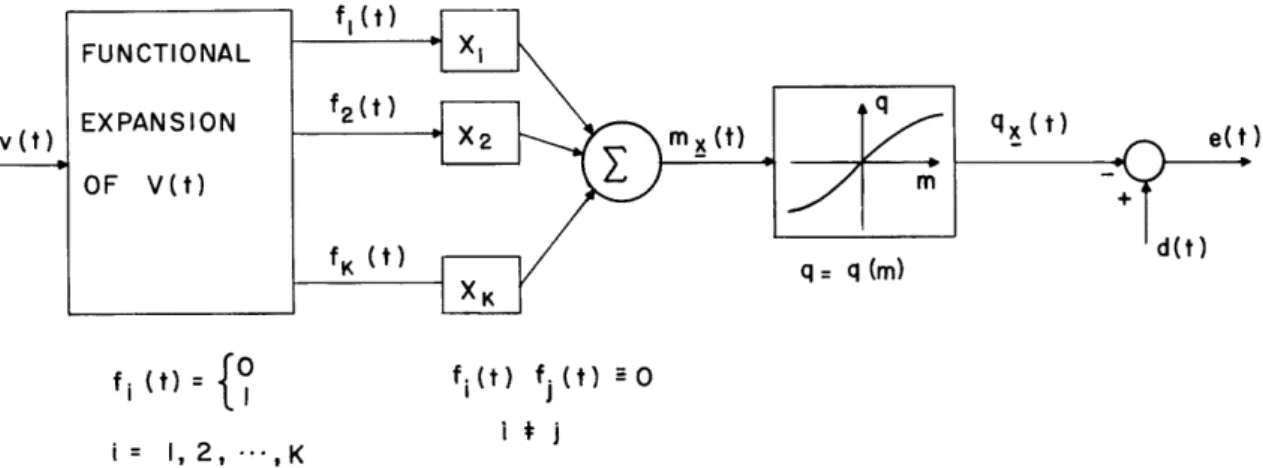
3. 3 BOSE FILTER FOLLOWED BY A NONLINEAR NO-MEMORY TRANSDUCER We consider the system shown in Fig. 5. A Bose nonlinear filter1 1

a nonlinear no-memory transducer that is described by the equation q(t) = g[m(t)] .

is followed by

(44) The functional expansion of the Bose filter may be of any form for which the functions fi(t) are orthonormal in the sense that

fi(t)= ( 26 (43) (45) K [n-1 6 (-j1- ) 5

j

Ih

hii .. - rn 1) -n- -,

fi(t) fj(t) - 0 i,j= 1,2,...k i j. (46) We assume that the nonlinear transducer is monotonic and satisfies the restriction

ag(m)

0 <K1 < am

< K2 for all m

(47) - M -< m -< M, with M = max xi|

i = 1,2,... ,k

x X

Only a slight modification of the proof given in section 3. 1 is necessary, in this case, to include a nonlinear transducer that satisfies (47). However, because of the

v(t (t)

'd(t) q =q (m)

fi (t) = I fi(t) fj(t) -0 i = 1, 2, ",K

Fig. 5. Bose nonlinear filter followed by a nonlinear no-memory transducer.

orthogonality requirement expressed by Eq. (46), the present case has two properties that deserve mention. First, we note that M(x) may be expressed as

k k

(48)

M( = M(xi ) = Z P(fi*O) E{W [ d-g(xi) I fi*0]},

i=l i=l

and hence the xi's may be adjusted independently of one another. The situation is thus reduced from one minimization problem in k variables to k minimization problems in one variable. Second, because of the orthogonality, restriction (c) reduces to

P{(fiI>D)

E > 0, or in view of Eq. 45, to

P{fiO0} > E > 0

D>0 i = 1, 2, . . . k, (49)

Inequality (49) serves to give us more insight into the meaning of restriction (c).

27 and EXPANSION OF V(t) -) i = 1, 2, . .. k.

3.4 THE ERROR CRITERION W(e) = e

Note that restrictions (d) and (e) both prohibit the use of the error function W(e) = e . It is true that, for all practical purposes, W(e) = e can be approximated by a polynomial of finite degree. To actually do this, however, would undesirably complicate carrying out the iterative procedure. The only reason for requiring W to be a polynomial was to be able to show that assumption (iii-a) followed from restriction (g). If we are con-cerned with the case in which independent data are used for each succeeding iteration, then Fn(Xl) - 0, and it is no longer necessary to restrict W to a polynomial. It will, instead, only be necessary to require that W possess continuous first and second derivatives and be strictly convex in order that assumptions (ii-a) and (ii-b) be satisfied. Thus, forgetting the convexity requirement for the moment, if we were interested in the criterion W(e) = e (and had independent data for each iteration) we could use some transducer that behaved as I e for all e other than those near zero and which possessed continuous first and second derivatives for e = 0 (for example, a rectifier).

The convexity requirement, however, is more troublesome. Although it would be easy to construct a device that behaved as e for large values of e, it would be difficult to build a device that approximates e but is still strictly convex. We note that, other than restriction (g), we have not placed restrictions on the signal d(t) except that it be uniformly bounded in magnitude. Although the function W(e) =

I

e is not strictly convex, it is still convex, that is,

W[ aa+(l-a)b] aW[ a] + (l-a) W[b] 0 a 1. < (50)

Now, if sgn(a) = -sgn(b), then for any W(e) satisfying (50) there exists an E greater than 0 so that, for min [I[al,b e > > 0,

W[aa+(l-a)b] - aW(a) + (l-a) W(b) - aEla-bI 0 c a 1/2

Hence, if we replace restriction (e) by the weaker condition expressed by Eq. 50, and restriction (c) by the stronger condition that there exist a D > 0 with the property that for all x E X

Psgn x ft

)

sgn ( E ifi t-

)

i= i=

(51) then we again obtain inequality (17), and assumption (ii-a) is still satisfied.

The condition expressed by (51) is quite untractable; it would be extremely difficult in a practical situation to ascertain whether or not it is satisfied. Nevertheless, the condition is reasonable enough that one might carry out the procedure for W(e) = el

I I SET INGS Y IVEX S YI +II-ylI

,y- IT C -V-1I L' -% TvY-., i M.(x,y) FOR W(e)= le

(a) _{M(x,y)=lxl+lI-x +}

(b)

0)

)NVEX DWABLE

M(x,y) FOR W(e)=+ [e le /2

M (X,y)= [IXI]112 + [-x]/2 + [y/+l] + Y11/2

(c )

Fig. 6. _{Plots of system performance for a simple example.}

29 y

-O

with a fair amount of confidence that the procedure would converge. For the Bose filter mentioned in section 3. 3, (51) reduces to

P (sgn[xi-d t] = -sgn [i-dt] min[ xi-dtl, 1I i-dt D xi- i = 1, 2, .. .,k.

3. 5 CONVEXITY OF THE ERROR WEIGHTING FUNCTION AND UNIQUENESS OF THE MINIMUM OF M(t)

In section 3. 1 we required that the function W(e) be strictly convex. The reason for this was to guarantee that our performance function, M(. =

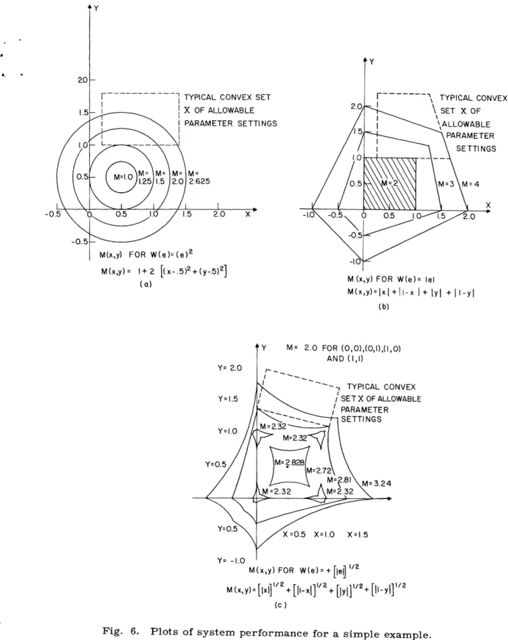
E{W[dt-qx t]} have only a unique minimum. The connection between the convexity of W and the uniqueness of the minimum of M(x) may be somewhat obscure. To clarify this point, we present a simple example. Consider two input signals sl(t) and s2(t) and a desired output signal d(t). We choose to estimate d(t) by q(t) = xs 1(t) + Ys 2(t).

If we assume the following probability distribution for sl, s2, and d, 1/4 s = 0, s2 = 1, d= 0 1/4 1 = 0, 2 = 1, d = 1 P(sl, s 2' d) = 1/4 s1 = 1, 2 = 0, d = 0 1/4 s₁ = 1 s2 = 0, d = 1 0 otherwise then

M(x, y) = 4E {Wd-xsl-ys₂]} = W[ x] + W[ l-x] + Wy] + W[1-y]

Figure 6 shows lines of equal average weighted error drawn in the x-y plane for the three error criteria W[ e] = e2, W[ e] = el, and W[ e] = + [lel] 1/2, respectively. Now 2 consider (x, y) as being restrained to a convex set X, in the x-y plane. For W(e) = e (which is strictly convex), there is clearly a unique minimum for any convex set, X, of parameter settings. The case W(e) = e| (which is only convex) is the dividing line; although for some choices of X, the minimum is not unique; nevertheless, all minima are connected and result in the same error. For W[ e] = + [ e 1/2, there are clearly choices of X for which there are separate minima. The four local minima in Fig. 6c happen to have the same average weighted error only because of the symmetry of P(s 1, s2, d).

IV. APPLICATIONS AND EXTENSIONS 4.1 A MORE GENERAL PERFORMANCE CRITERION

We have considered the optimum parameter setting to be that setting which mini-mized the performance function

M(x) = E{W[dt-qx, t]}

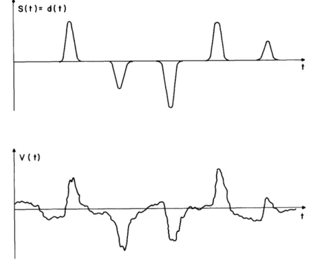
in which W may be any non-negative strictly convex weighting function on the error. This implies that the error is equally harmful under all situations (we are referring to situations that are distinct from the value of the error). In certain applications the error will be more harmful when certain conditions on the input and desired output exist. An example of this is found in the transmission of pulses as shown by the waveforms of Fig. 7. The signal s(t) consists of a train of periodic pulses that have been corrupted by a continuous noise signal to form the signal v(t). The actual purpose of the filter is to recover the height of the pulses; however, minimization of the performance function M() requires that the filter also do a good job of smoothing out the noise between pulses. As pointed out by Bose, this requirement may impair the filter's ability to recover the pulses. S(t)= d(t)

A

V

A

t V ( t)

Fig. 7. Pulse-transmission waveforms.

In cases of this kind it would be more-meaningful to minimize the performance function 31 I I- -r n

M() = E 1 [dt tW2[vt-T VtT dt- ' dtm]

O < T1 < T2 < ...< < o (52) in which W1 is again a non-negative strictly convex function, and W2 is an appropriate bounded non-negative function. The use of this type of performance function does not greatly complicate the iterative adjustment procedure. In the example discussed above, it would only be necessary to carry out the adjustments at those times when a pulse is being transmitted in order to minimize the performance function

M(x) = E{W1[dt-qx, t] W [dt]} in which

I d(t) * 0

W2[d(t)] = d(t)

d(t) 0.

However, we must still show that the adjustment procedure converges for perform-ance criteria of the type expressed by Eq. 52. In establishing assumptions (i) and (ii),

we estimated upper and lower bounds on certain averages of Wl[d(t)-qx(t)]. Thus if

0 < K1 < W2 K2 < 0, (53)

then these estimates could still be obtained by taking W Z outside of the averaging

opera-tion. If

o0 WZ K < 00, (54)

then it is only necessary to strengthen restriction (c) to read

(c') P _(C) 1_PW d t- X ..

2

[v. vt-Tm dt-1 t t-Tm] (x n i t -i)fi, > DI x

-l

a E > 0 for all x E X D> 0

in order for the preceding work establishing assumption (ii-a) to still be valid.

The work of sections 3.1 and 3. 2 establishing the validity of assumption (iii-a') also remains valid, with the exception that the estimate of Fn(Xl) now becomes

F (l/Z)(n-Tm

F (x,) K (55)

n C(1/2) (n-Tm)

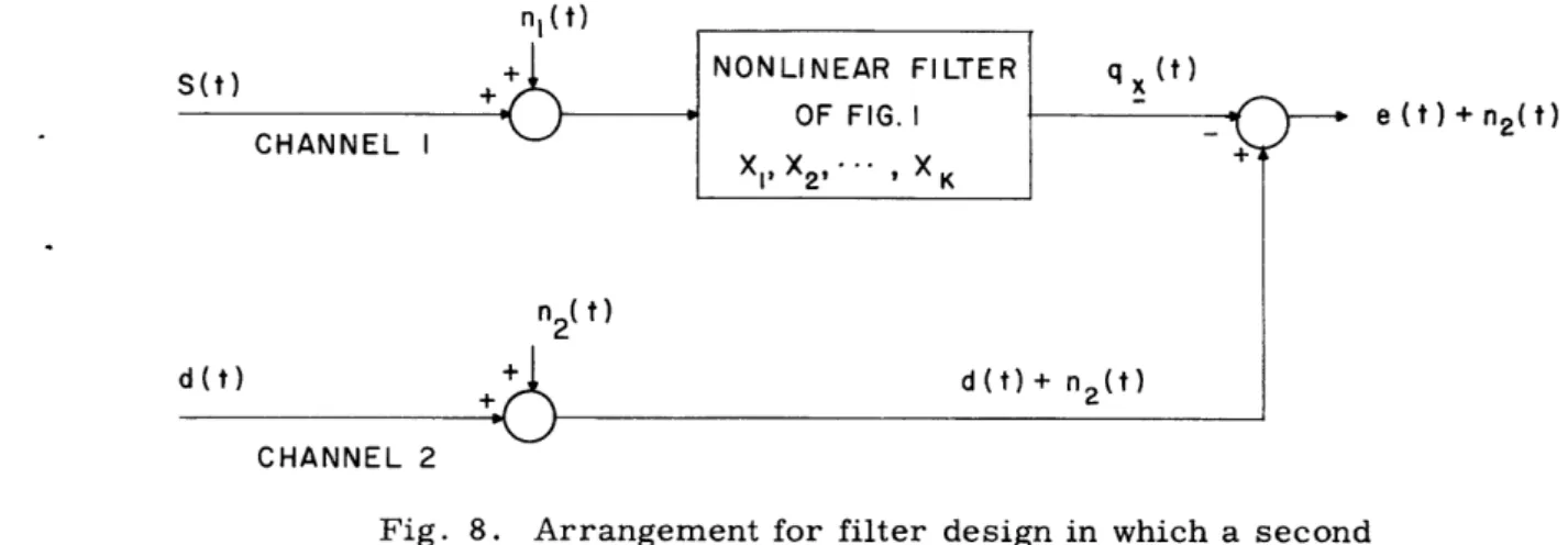
4.2 DESIGN OF A FILTER WHEN A SECOND INDEPENDENT CHANNEL IS

AVAILABLE

In the design of a filter the uncorrupted signal, d(t), is generally not available. One way of circumventing this problem is to use a record of the data v(t) and d(t). If a