HAL Id: hal-01349737
https://hal.archives-ouvertes.fr/hal-01349737
Submitted on 28 Jul 2016HAL is a multi-disciplinary open access archive for the deposit and dissemination of sci-entific research documents, whether they are pub-lished or not. The documents may come from teaching and research institutions in France or abroad, or from public or private research centers.
L’archive ouverte pluridisciplinaire HAL, est destinée au dépôt et à la diffusion de documents scientifiques de niveau recherche, publiés ou non, émanant des établissements d’enseignement et de recherche français ou étrangers, des laboratoires publics ou privés.
Combining punctual and ordinal contour data for
accurate floodplain topography mapping
Carole Delenne, Jean-Stéphane Bailly, Mathieu Dartevelle, Nelly Marcy,
Antoine Rousseau
To cite this version:
Carole Delenne, Jean-Stéphane Bailly, Mathieu Dartevelle, Nelly Marcy, Antoine Rousseau. Combin-ing punctual and ordinal contour data for accurate floodplain topography mappCombin-ing. Spatial Accuracy 2016, Jean-Stéphane Bailly; Didier Josselin, Jul 2016, Montpellier, France. pp.350-357. �hal-01349737�
Combining punctual and ordinal contour data for accurate floodplain
topography mapping
Carole Delenne*1,3, Jean-St´ephane Bailly2, Mathieu Dartevelle3, Nelly Marcy1, Antoine Rousseau3 1Univ. Montpellier, HSM, France
2AgroParisTech, LISAH, France 3INRIA, Lemon, France
*Corresponding author: [email protected]
I INTRODUCTION
Hydrodynamic models in two dimensions require a precise knowledge of the domain topog-raphy. However, as far as the modelling of great rivers or lakes is concerned, few accurate topographic records are generally available to accurately model the floodplain topography. The usual way to acquire accurate topographic information for hydraulics over floodplain remains the ground surveys, that provide punctual values at a very high cost. Based on these points, usual interpolation schemes often yield a too coarse and inaccurate topographic map for a re-alistic hydrodynamic modelling. Remote sensing data such as Lidar or stereo-photogrammetry data on non vegetated areas, constitute a good alternative to obtain large scale information, but yield other issues of acquisition and data processing. In addition, topographic Lidar operat-ing with near-infrared lasers are still not suitable for an exhaustive survey of floodplains where submerged areas remain.
Progress in remote sensing data repeatability and spatial resolution now allows the automatic monitoring of water surfaces delineation from areal or satellite images either in optical or radar
domains (see e.g. an application to the Inner Niger Delta in Ogilvie et al.(2015)). As for the
recently launched Sentinel sensors, these data are becoming widely available with increasing spatial and temporal resolutions, allowing in turn the spatio-temporal monitoring of flooded areas. Flood dynamics from remote sensing data are known to be informative on floodplain
topography for long (see e.g. Schumann et al. (2007) orHostache et al. (2010)). Indeed, the
extracted flooded areas may be considered as iso-elevation contour lines, as the hypothesis can be made that all the points located on the water/soil limit have the same elevation. If contour line elevation remains unknown, rank between the detected contour lines as well as between every contour line and surrounding topographic data points are known. Assuming this information, the next challenge is thus to develop a spatial data fusion method of ordered contour lines data and usual elevation data points to better model the floodplain topography.
Mixing punctual ranked and continuous data in spatial estimation was already proposed in
liter-ature, mainly to deal with highly skewed field distribution (Yamamoto,2000) or for very large
spatial datasets (Cressie and Johannesson,2008). These methods used the uniform score
trans-form and back-transtrans-form based on the standardized rank estimation (Saito and Goovaerts,2000)
to prevent the right estimate distribution and limit the smoothing effect of kriging. Uncertainty assessment of resulting punctual kriging estimates was proposed thanks to the transformation
process (Yamamoto, 2007). Other methods also exist to quantify the uncertainty of contour
lines in random fields (Lindgren and Rychlik, 1995; Wameling and Saborowski, 2001). But
in these studies, the objective was to quantify the uncertainty in contour lines location and not to quantify the uncertainty of contour lines level for a known location. Consequently, these
different studies only partly touched the problem we face.
The objective of this paper is to propose a method to estimate the elevation of the ranked contour lines from data points. This method starts from block conditional simulations estimates filtered on rank statistics. After contour line elevation estimate, a usual kriging is performed to recon-struct a topographic map over the floodplain. Starting from a synoptic and theoretical example, the principles, advantages, properties and limitations of the proposed method are exposed. The spatial accuracies obtained in contour lines estimates and topographic map are thus compared to the usual block kriging estimates.
II MATERIAL AND METHODS
2.1 Case study generation
A reference exhaustive elevation field Z(s) on a floodplain D was generated from a Gaussian spatial covariance model with range 20, sill 1 and no nugget effect. The resulting field is
centered on µ = 10 and respects distribution N (µ, σ) (see Figure 1-left): the blue colours
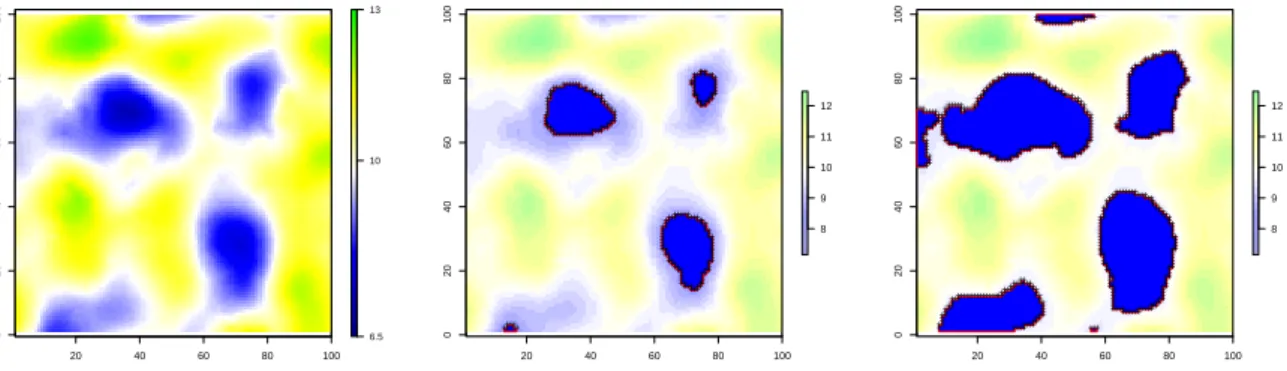
represent lower floodplain elevations meanwhile the yellow and green stem for higher elevation areas. D is a 100 m×100 m area and the dataset was generated on gridded D with resolution r = 1 m, r denoting both the remote sensing image spatial resolution and the desired end-user topographic map resolution.
20 40 60 80 100 0 20 40 60 80 100 6.5 10 13 20 40 60 80 100 0 20 40 60 80 100 8 9 10 11 12 ++ +++++ + + + + + + + + + + + + + + + + + + + + + + + + + + + + + + + + + + + + ++++++++++++++++++++++++++++++++++++++++++++ + + + + + + + + + + + + ++++++++++++++++++++++++++ + + + + + + + + + + + + + + + + ++++++++++++++++++++++++++++++++++++++++++++++++++++++++++++ 20 40 60 80 100 0 20 40 60 80 100 8 9 10 11 12 ++ + + + + + + + + + + + +++++++++++++++++++++++++++++++++++++++++++++++++++++++++++++++ +++ + + + + + + + + + + + + + +++ + + + + + + + + + + + + + + + + + + + + + + +++++++++++++++++++++++++++++++++++++++++++++++++++++++++++++++++++++++++++++++++++++ + + + + + + + + + + + + + + + ++++++++ + + + + + + + + + + + + + + + + ++++++++++++++++++++++++++++++++++++++++++++++++++++++++++++++++++++++++++++++++++++ + + + + + + + + + + + + + + + + ++++++++++++++++++++++++++++++++++++++++++++++++++++++++++++++++++++++++++++++++++++++++++++++++++++++++++++++++++++++++++++++++++++++++++++++++ + + + + +++++++++++++++++++++++++++++++
Figure 1: Generated case study. Left: Simulated elevation field over D; Middle: flooded area at time 1 (blue) and resulting rasterized contour (black crosses); Right: flooded area at time 2 (blue) and resulting rasterized contour (black crosses).
To reproduce the remote sensing data support (Ogilvie et al., 2015), flooded areas were
gen-erated and delineated at resolution 0.5 m for two different times t1 and t2 during rising water:
when areas lower than 9.5 m (Fig. 1-middle) and 8.5 m (Fig.1-right) respectively are flooded.
Contour polylines were generated from these rasterized flooded areas with 0.5 m spatial
reso-lution. The sets of two generated contour polylines C1 and C2 were thus reduced to a set of
polylines vertices sji (j ∈ (1, 2) denoting the polyline) regularly located along the lines (black
cross on figures 1). C1 and C2 contained n1 = 201 and n2 = 520 points respectively. Four
contour lines correspond to C1 and five to C2 (Fig. 1). When contour lines were connected to
the D boundaries, only vertices within D were considered.
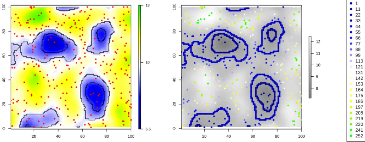
In addition, a sample of n = 250 topographic points s1. . . sn was randomly selected on D,
excluding points selection at location closer than b = 2 m from polylines (Fig.2-left). This
of its elevation. We further assume that contour polylines elevation is unknown but that ranks
between the polylines (i.e. the polyline vertices sji) and between polylines and surrounding
topographic data points are known and may be computed (Fig. 2-right).
20 40 60 80 100 0 20 40 60 80 100 6.5 10 13 ● ● ● ● ● ● ● ● ● ● ● ● ● ● ● ● ● ● ● ● ● ● ● ● ● ● ● ● ● ● ● ● ● ● ● ● ● ● ● ● ● ● ● ● ● ● ● ● ● ● ● ● ● ● ● ● ● ● ● ● ● ● ● ● ● ● ● ● ● ● ● ● ● ● ● ● ● ● ● ● ● ● ● ● ● ● ● ● ● ● ● ● ● ● ● ● ● ● ● ● ● ● ● ● ● ● ● ● ● ● ● ● ● ● ● ● ● ● ● ● ● ● ● ● ● ● ● ● ● ● ● ● ● ● ● ● ● ● ● ● ● ● ● ● ● ● ● ● ● ● ● ● ● ● ● ● ● ● ● ● ● ● ● ● ● ● ● ● ● ● ● ● ● ● ● ● ● ● ● ● ● ● ● ● ● ● ● ● ● ● ● ● ● ● ● ● ● ● ● ● ● ● ● ● ● ● ● ● ● ● ● ● ● ● ● ● ● ● ● ● ● ● ● ● ● ● ● ● ● ● ● ● ● ● ● ● ● ● ● ● ● ● ● ● ● ● ● ● ● ● 20 40 60 80 100 0 20 40 60 80 100 8 9 10 11 12 ●● ●●●●● ● ● ● ● ● ● ● ● ● ● ● ● ● ● ● ● ● ● ● ● ● ● ● ● ● ● ● ● ● ● ● ● ● ● ● ● ●●●●●●●●●●●●●●●●●●●●●●●●● ● ●●●●●●●●● ● ● ● ● ● ● ● ● ● ● ● ● ● ● ● ● ● ● ● ● ● ●●●●●●●●●●●●●●●●●●●●●●● ● ● ● ● ● ● ● ● ● ● ● ● ● ● ● ● ● ● ● ●●●●●●●● ● ● ●●●●●●●●●●●●●●●●●●●●●●●● ●●●●●●●●●●●●●● ● ● ● ● ● ● ● ● ● ● ● ● ●● ● ● ● ● ● ● ● ● ● ● ● ●●●●●●● ●●●●●●●●●●●●●●●●●●●●●●●●●●●●●●●●● ●●●●● ●●●●●●●●●●●●● ● ● ● ● ● ● ● ● ● ● ● ● ● ● ● ● ● ● ● ● ● ●●● ● ● ● ● ● ● ● ● ● ● ● ● ● ● ● ● ● ● ● ● ● ● ●●●●●●● ●●●●●●●●●●●●●●●●●●●●●●●● ●●●●●●●●●●●●● ● ●●●●●● ● ● ● ● ● ● ● ● ● ● ● ● ● ● ● ● ● ● ● ● ● ● ● ● ● ● ● ● ● ● ● ● ● ● ● ● ● ● ● ● ● ● ● ● ● ● ● ● ● ●●●●●●●● ● ● ● ● ● ● ● ● ● ● ● ● ● ● ● ● ●●●●●●●●●●●●● ● ● ● ● ● ● ● ●●● ●●●●●●●●●●●●●●●●●●●●●●●●●●●●● ● ●●● ● ● ● ● ● ● ● ● ● ● ● ● ● ● ● ● ● ● ● ● ● ● ● ● ● ● ● ● ● ● ● ● ● ● ● ● ● ● ● ● ● ● ● ● ●●●●●●●●●●●●●●●●●●●●●● ●●●●●●●●●●●●●●●●●●●●●●●●●●●●●●●●●●●●●●●●●●●●●●● ●●●●●●●●●●●● ● ● ● ● ● ● ● ● ● ● ● ● ● ● ● ● ● ● ● ● ● ● ● ● ● ● ● ● ● ● ● ● ● ● ● ● ● ● ● ● ● ● ● ● ● ● ● ● ● ● ● ● ● ● ● ● ● ● ● ● ● ● ● ● ● ● ● ●●●●●●●●●●●●●● ● ● ● ● ● ● ● ●●●●●● ●●●● ● ● ● ● ● ● ● ● ● ● ● ● ● ● ● ● ● ● ● ● ● ● ● ● ● ● ● ● ● ● ● ● ● ● ● ● ● ● ● ● ● ● ● ● ● ● ● ● ● ● ● ● ● ● ● ● ● ● ● ● ● ● ● ● ● ● ● ● ● ● ● ● ● ● ● ● ● ● ● ● ● ● ● ● ● ● ● ● ● ● ● ● ● ● ● ● ● ● ● ● ● ● ● ● ● ● ● ● ● ● ● ● ● ● ● ● ● ● ● ● ● ● ● ● ● ● ● ● ● ● ● ● ● ● ● ● ● ● ● ● ● ● ● ● ● ● ● ● ● ● ● ● ● ● ● ● ● ● ● ● ● ● ● ● ● ● ● ● ● ● ● ● ● ● ● ● ● ● ● ● ● ● ● ● ● ● ● ● ● ● ● ● ● ● ● ● ● ● ● ● ● ● ● ● ● ● ● ● ● ● ● ● ● ● ● ● ● ● ● ● ● ● ● ● ● ● ● ● ● ● ● ● ● ● ● ● ● ● ● ● ● ● ● ● ● ● ● ● ● ● ● ● ● ● ● ● ● ● ● ● ● ● ● ● ● ● ● ● ● ● ● ● ● ● 1 11 22 33 44 55 66 77 88 99 110 121 131 142 153 164 175 186 197 208 219 230 241 252
Figure 2: Generated dataset. Left: Simulated elevation field over D, contour polylines C1 and C2 (black lines) and data points (red points). Right: ranked data (points and polyline vertices) and according legend.
2.2 Method
The method we developed may be seen as a block conditional simulation process filtered by
rank statistics, where a polyline Cj is seen as a block, i.e. a region corresponding to an
uncon-nected set of vertices. Such simulation is known to be superior to kriging whenever interest lies in global statements for a region rather than inference on individual points. In the process
described in the algorithm1hereafter, assuming a stationary random function, a spatial model
(variogram) γ(h) is first estimated and modelled from the 250 data points s1. . . sn.
Algorithm 1 Contour polyline estimation process and field reconstruction
1: for j = 1 to j= 2 do
2: Estimate and model the variogram γ(h) from n data points
3: Estimate ordinary kriging ˆzko(sji) on polyline vertices
4: for i = 1 to N = 100 do
5: Draw unconditional multigaussian simulation zus(sk) and zus(s
j
i) on data location
and polyline vertices
6: Estimate ordinary kriging at vertices from simulated values at data locations zko∗ (sji)
7: Compute conditional simulation on vertices (Eq. 1)
8: Compute N polyline estimate by averaging vertices conditional simulations
9: Filter keeping only polyline estimate conform to the initial ranks
10: Compute polyline estimate ˆzj averaging the kept polyline estimates
11: Compute standard deviation estimate from the set of kept polyline estimates
12: Affect polyline estimate ˆzj to each polyline vertice sji
13: Perform ordinary kriging on all gridded D points from data z(s1) · · · z(sn) and polyline
Once the variogram γ(h) is modelled, an ordinary kriging is performed on each polyline ver-tex. From the kriging, a first estimate of polyline elevation results from vertices averaging.
For polyline Cj, we denote further ˆzkoj this estimate (corresponding to the usual block kriging
estimate).
Next, a set of N = 100 conditional Multi-Gaussian simulations using the fitted variogram
model and pathing through the 250 s1. . . sn is performed on each on the sji contour vertices
(Eq. 1): zcs(sji) = ˆzko(sji) + (zus(sji) − ˆz ∗ ko(s j i)) (1)
At the end of the conditional simulation, an estimate at polyline scale is computed by averaging simulated values on vertices. This remains consistent with the usual block kriging estimate since vertices are regularly located along the polyline.
ˆ zkj = 1 nj nj X i=1 zcs(s j i) (2)
We thus obtain N elevation estimates ˆzkj, k ∈ (1 . . . N ) for a given contour polyline Cj. Only the
estimates respecting the rank are kept in the following, yielding a set of M estimates (M ≤ N )
for a given polyline. From this set, the final estimate of polyline Cj becomes:
ˆ zj = 1 M M X k=1 ˆ zkj (3)
with uncertainty characterized by the standard deviation σCj of the ˆz
j
kestimates.
In a final step, polyline estimate ˆzj is affected to each polyline vertex sji in order to perform, in
addition to the 250 data points a gridded map using ordinary kriging.
III RESULTS
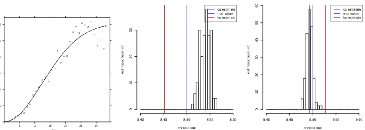
Results obtained for this theoretical test case are given in Figures3and4. Figure3-left shows
the estimated empirical variogram (dots) and fitted variogram model (lines). Figure 3-right
shows for C1 and C2the resulting distribution of the estimates using conditional simulation, the
final estimation equal to the average of conditional simulation (black vertical line) compared to the true value (blue vertical line) or the ordinary kriging (interpolation) estimate (red vertical line). In this first application, rank was always respected in the conditional simulation and for the ordinary kriging but, as shown in the following, this will not always be the case. The
estimated elevation obtained for C1 is 8.53 m (8.45 using ordinary kriging) for a true value
equals to 8.5 m, with a standard deviation of the estimate being only 5.37e-03 m. For C2,
the difference between the true elevation (9.5 m) and the estimated value is lower than one centimetre (3 cm using kriging) with standard deviation of the estimate equals to 3.99e-03 m.
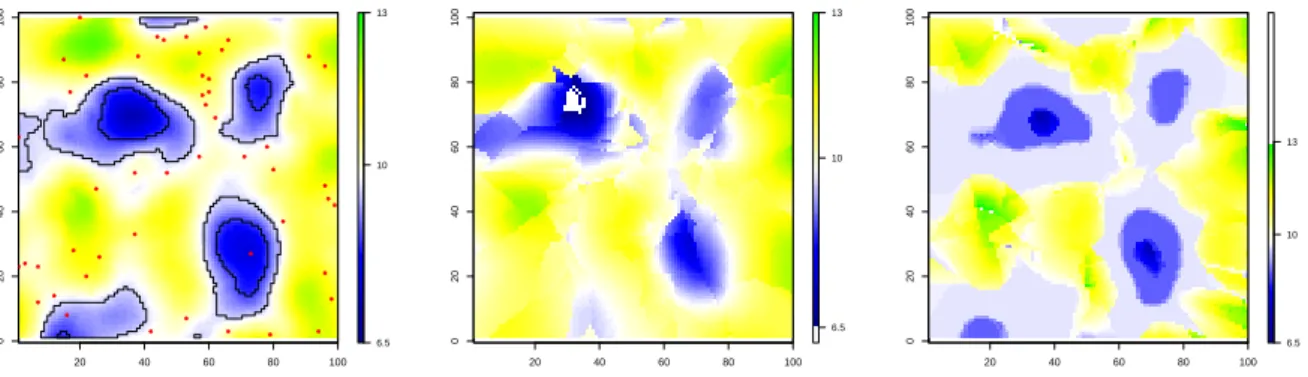
Figure4 shows the reconstructed fields from the method we proposed compared to i) the true
field and ii) the field reconstructed only from the 250 data points without considering the contour polylines data. A visual comparison suggests better results for the proposed approach. However, artefacts can bee seen around the pool located at the bottom-right corner of the domain. In this area, the elevation increases with the distance to the pool minimum but decreases again at
distance semiv ar iance 0.2 0.4 0.6 0.8 1.0 1.2 5 10 15 20 25 30 ● ● ● ●● ● ● ● ● ● ● ● ● ● ● ● ● ● ● ●● ● ● ● ● ● ● ● ● ● ● ● ● ● contour line estimated le v el (m) 8.40 8.45 8.50 8.55 8.60 0 10 20 30 cs estimate true value ko estimate contour line estimated le v el (m) 9.40 9.45 9.50 9.55 9.60 0 10 20 30 40 50 60 cs estimate true value ko estimate
Figure 3: Left: Re-estimated empirical variogram from the n = 250 data points; Right: estimated elevation for C1 and C2.
three places. This behaviour can be explained by the fact that very few topographic points are available around this pool.
On the contrary, the field reconstructed with the ordinary kriging method shows greater differ-ence to the true field especially on the top part of the domain, despite a high concentration of ground-truth surveys.
To better assess the precision given by the two approaches, the root mean square difference e between results and true field is computed. The error value obtained without considering the contour polylines is equal to 0.232 m, and to 0.199 m for the proposed method.
20 40 60 80 100 0 20 40 60 80 100 6.5 10 13 20 40 60 80 100 0 20 40 60 80 100 6.5 10 13 20 40 60 80 100 0 20 40 60 80 100 6.5 10 13
Figure 4: Reconstructed elevation fields: Left: true field D; Middle: ordinary kriging reconstructed field; Right: method (polyline conditional simulation) reconstructed field
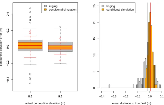
This first test suggests that the sampling procedure may influence the results, at least through the location of acquisition points. To check the robustness of the proposed approach, the process described above was repeated 100 times, changing the 250 points data sampling.
Figure5-left shows the contour polyline C1 and C2 error distribution obtained. Figure 5-right
shows the mean distance to the true field distribution. Clearly, the proposed method using conditional simulation is more robust with few error variance. The standard deviation of the results obtained with this approach is 0.056 m (resp. 0.037 m) for the contour line 8.5 (resp. 9.5) compared to 0.183 m (resp. 0.1 m) using the ordinary kriging method.
Rank filtering occurred 10% of the times for the C1 estimation and never for the C2estimation.
This suggests that rank filtering is useful when contours are in extreme values.
● ● ● ● ● ● ● ● ● ● ● ● ● ● 8.5 9.5 −0.4 −0.2 0.0 0.2 0.4
actual contourline elevation (m)
contour line ele v ation error (m) ● ● ● ● 8.5 9.5 −0.4 −0.2 0.0 0.2 0.4 kriging conditional simulation
mean distance to true field (m)
−0.4 −0.3 −0.2 −0.1 0.0 0.1 0 5 10 15 20 25 kriging conditional simulation
Figure 5: Errors distribution on 100 random sample sets of 250 data points. Left: Cj estimation error; Right : mean distance to the true field after reconstruction. The vertical lines represent the mean of the distribution.
Field survey being very costly, the aim is to reduce to the minimum the required elevation data points. The test is thus performed again with different numbers of points. An example of result
obtained with a random sample of N = 50 points is given in Figure6. It can be seen that the
use of contour line enables to retrieve the pools shapes with better accuracy than an ordinary kriging based only on data points.
The comparison between true field and computed elevation fields with the two approaches is
done using the root mean square error. These results are summarized in Table 1 for random
samples obtained with N = 10 to N = 250. As expected, the error decreases if the number of available data points is high and the proposed approach always gives better results than the ordinary kriging.
N = 10 N = 50 N = 100 N = 150 N = 200 N = 250
eko 1.064 0.635 0.361 0.403 0.435 0.232
ecs 0.639 0.469 0.329 0.227 0.189 0.199
20 40 60 80 100 0 20 40 60 80 100 6.5 10 13 ● ● ● ● ● ● ● ● ● ● ● ● ● ● ● ● ● ● ● ● ● ● ● ● ● ● ● ● ● ● ● ● ● ● ● ● ● ● ● ● ● ● ● ● ● ● ● ● ● ● 20 40 60 80 100 0 20 40 60 80 100 6.5 10 13 20 40 60 80 100 0 20 40 60 80 100 6.5 10 13
Figure 6: Reconstructed elevation fields using only 50 data points: Left: true field D; Middle: ordi-nary kriging reconstructed field; Right: method (polyline conditional simulation) reconstructed field.
IV DISCUSSION AND CONCLUSION
The objective of this work was to put forward a methodology to enhance the accuracy of the topographic description required by numerical hydrodynamic modelling, by using information of level lines available from remote-sensing data.
The first results obtained on a totally theoretical example, show that the topographic estimation benefits from such additional data; and the repetition of the process indicates that this result is robust to sampling. If the gain in accuracy may seem limited at this stage (about 3 cm in mean for 250 points), the influence of the sampling rate should be assessed more precisely on the two approaches, since the benefit taken from additional sources of information is expected to increase as less ground-truth data are available.
Moreover, a classical random sampling is obviously not the best approach to conduct a field survey. In the first presented test case, random sampling excluding the direct neighbourhood of the contour lines yielded a lack of data near the pool located at bottom-right part of the domain. This produced irrelevant estimation of the topography in some areas. Further tests are thus planed to infer guidelines in the sampling definition in order to decrease the number of data points required while maintaining a high accuracy in the results, thus enhancing the cost/benefice ratio. In the framework of hydrodynamic modelling, this work will integrate
results of uncertainty and sensitivity analyses such as given inGuinot and Cappelaere(2009) or
Delenne et al.(2012).
The methodology developed on theoretical test cases, will be assessed in a real-case study of the hydrodynamic modelling of the Vaccares lagoon for which amount of data are available for validation.
References
Cressie N., Johannesson G. (2008). Fixed rank kriging for very large spatial data sets. Journal of the Royal Statistical Society: Series B (Statistical Methodology) 70(1), 209–226.
Delenne C., Cappelaere B., Guinot V. (2012). Uncertainty analysis of river flooding and dam failure risks using local sensitivity computations. Reliability Engineering and System Safety 107, 171–183.
Guinot V., Cappelaere B. (2009). Sensitivity equations for the one-dimensional shallow water equations: Practical application to model calibration. Journal of Hydrologic Engineering 14, 858–861.
Hostache R., Lai X., Monnier J., Puech C. (2010). Assimilation of spatially distributed water levels into a shallow-water flood model. part ii: Use of a remote sensing image of mosel river. Journal of Hydrology 390(3-4), 257 – 268.
Lindgren G., Rychlik I. (1995). How reliable are contour curves? confidence sets for level contours. Bernoulli, 301–319.
Ogilvie A., Belaud G., Delenne C., Bader J.-C., Oleksiak A., Bailly J. S., Ferry L., Martin D. (2015). Decadal monitoring of the Niger Inner Delta flood dynamics using MODIS optical data. Journal of Hydrology 523, 358–383.
Saito H., Goovaerts P. (2000). Geostatistical interpolation of positively skewed and censored data in dioxin-contaminated site. Environmental Science Technology 34, 4228–4235.
Schumann G., Matgen P., Hoffmann L., Hostache R., Pappenberger F., Pfister L. (2007). Deriving distributed roughness values from satellite radar data for flood inundation modelling. Journal of Hydrology 344(1-2), 96 – 111.
Wameling A., Saborowski J. (2001). Construction of local confidence intervals for contour lines. In Proceedings of the IUFR4.11 Confererence in forest biometry.
Yamamoto J. K. (2000). An alternative measure of the reliability of ordinary kriging estimates. Mathematical Geology 32, 489–509.
Yamamoto J. K. (2007). On unbiased back-transform of lognormal kringing estimates. Computacional Geo-sciences 11, 219–234.