HAL Id: hal-02154926
https://hal.archives-ouvertes.fr/hal-02154926
Submitted on 16 Dec 2019
HAL is a multi-disciplinary open access
archive for the deposit and dissemination of sci-entific research documents, whether they are pub-lished or not. The documents may come from teaching and research institutions in France or
L’archive ouverte pluridisciplinaire HAL, est destinée au dépôt et à la diffusion de documents scientifiques de niveau recherche, publiés ou non, émanant des établissements d’enseignement et de recherche français ou étrangers, des laboratoires
Kernelizations for the hybridization number problem on
multiple nonbinary trees
Leo van Iersel, Steven Kelk, Celine Scornavacca
To cite this version:
Leo van Iersel, Steven Kelk, Celine Scornavacca. Kernelizations for the hybridization number problem on multiple nonbinary trees. Journal of Computer and System Sciences, Elsevier, 2016, 82 (6), pp.1075-1089. �10.1016/j.jcss.2016.03.006�. �hal-02154926�
Kernelizations for the hybridization number problem
on multiple nonbinary trees
ILeo van Iersela,1, Steven Kelkb, Celine Scornavaccac
aDelft Institute of Applied Mathematics, Delft University of Technology, P.O. Box 5, 2600 AA
Delft, The Netherlands
bDepartment of Knowledge Engineering (DKE), Maastricht University, P.O. Box 616, 6200 MD
Maastricht, The Netherlands
cISEM, CNRS – Universit´e Montpellier II, Place Eug`ene Bataillon, 34095, Montpellier, France
Abstract
Given a finite set X, a collection T of rooted phylogenetic trees on X and an integer k, the Hybridization Number problem asks if there exists a phylogenetic network on X that displays all trees from T and has reticulation number at most k. We show two kernelization algorithms for Hybridization Number, with kernel sizes 4k(5k)t and 20k2(∆+ − 1) respectively, with t the number of input trees and ∆+
their maximum outdegree. Experiments on simulated data demonstrate the practical relevance of our kernelization algorithms. In addition, we present an nf (k)t-time algorithm, with n = |X| and f some computable function of k.
Keywords: Fixed-parameter tractability, kernelization, phylogenetic tree, phylogenetic network, hybridization number
IA preliminary version of this article appeared in the proceedings of Workshop on
Graph-Theoretic Concepts in Computer Science (WG 2014).
Email addresses: [email protected] (Leo van Iersel),
[email protected] (Steven Kelk), [email protected] (Celine Scornavacca)
1Leo van Iersel was partially funded by a Veni grant from The Netherlands Organisation for
1. Introduction
In phylogenetics, one central challenge is to construct a plausible evolutionary history for a set of contemporary species X given incomplete data. This usually concerns biological evolution, but the paradigm is equally applicable to more abstract forms of evolution, e.g. natural languages [24]. Classically an evolutionary history is modelled by a rooted phylogenetic tree, essentially a rooted tree in which the leaves are bijec-tively labelled by X [26]. In recent years, however, there has been growing interest in generalizing this model to directed acyclic graphs, that is, to rooted phylogenetic networks [2, 11, 23]. In the latter model, reticulations, which are vertices of inde-gree 2 or higher, are of central importance; these are used to represent non-treelike evolutionary phenomena such as hybridization and lateral gene transfer. The reticu-lation number of a phylogenetic network can be defined as the number of edges that need to be removed in order to obtain a tree. It is easy to see that in networks with maximum indegree 2 (to which we will be able to restrict without loss of generality) the reticulation number is simply equal to the number of reticulations. This setting has naturally given rise to the Hybridization Number problem: given a set of rooted phylogenetic trees T on the same set of taxa X, construct a rooted phylo-genetic network on X with the smallest possible reticulation number, such that an image of every tree in T is embedded in the network [3].
Hybridization Number has attracted considerable interest in a short space of time. Even in the case when T consists of two binary (that is, bifurcating) trees the problem is NP-hard, APX-hard [5] and in terms of approximability is a surpris-ingly close relative of the problem Directed Feedback Vertex Set [17, 13]. On the positive side, this variant of the problem is fixed-parameter tractable (FPT) in parameter k, the reticulation number of an optimal network. Initially this was established via kernelization [6], but more recently efficient bounded-search algo-rithms have emerged with O(3.18k· poly(n)) being the current state of the art [28], with n = |X|.
In this article we focus on the general case when t = |T | ≥ 2 and the trees in T are not necessarily binary. This causes complications for two reasons. First, when t > 2, the popular “maximum acyclic agreement forest” abstraction breaks down, a central pillar of algorithms for the t = 2 case. Second, in the nonbinary case the images of the trees in the network are allowed to be more “resolved” than the original trees. (More formally, an input tree T is seen as being embedded in a network N if T can be obtained from a subgraph of N by contracting edges.) The reason for this is that vertices with outdegree greater than two are used by biologists to model uncertainty in the order that species diverged. Both factors complicate matters considerably. Consequently, progress has been more gradual.
For the case of multiple binary trees, there exists a kernel with at most 20k2leaves [15], various heuristics [7, 8, 29] and an exact approach without running-time bound [30]. For the case of two nonbinary trees, there is also a polynomial kernel [20], based on a highly technical kernelization argument, and a simpler FPT algorithm based on bounded search [25].
This leaves the general case of multiple nonbinary trees as the main variant for which it is unclear whether the problem is FPT. The most obvious parameter choice is, as before, the reticulation number k. However, other natural parameters in this case are the number of input trees t and the maximum outdegree ∆+ over all input trees. By the NP-hardness result mentioned above, it is clear that Hybridization Number is not FPT if the parameter is t or ∆+, unless P = NP. Therefore, the most interesting
questions are whether the problem is FPT if either (a) the only parameter is k, or (b) there are two parameters: k and t, or (c) there are two parameters: k and ∆+.
In this paper, we answer the latter two questions affirmatively, using a kerneliza-tion approach. First, we prove that Hybridization Number admits a kernel with at most 4k(5k)t leaves. Second, we show a slightly different kernel with at
most 20k2(∆+ − 1) leaves. The running time of both kernelization algorithms is polyomial in n and t. Whether Hybridization Number remains FPT if k is the only parameter remains open. However, we do present an algorithm for Hybridiza-tion Number that runs in nf (k)t time, with f some computable function of k, hence showing that the problem is in the class XP.
Similar results can alternatively be obtained using bounded-search algorithms instead of kernelization, see the e-print [18]. We do not include those algorithms here because the proofs (although based on several important insights) are highly technical and the running times astronomical. In contrast, the kernelization algorithms are simple, fast and their proofs relatively elegant. Therefore, we only include the last result of
our e-print [18], which is the O(nf (k)t) time algorithm, in this paper. Its running
time is also astronomical but, combined with the kernelization algorithms, it gives explicit FPT algorithms, which are (theoretically) the best known algorithms that can solve general instances of Hybridization Number.
Some of the lemmas that we prove in order to derive the correctness of the kerneliza-tion algorithms are of independent interest because they improve our understanding of how nonbinary trees can be embedded inside networks. This helps us to avoid a technical case analysis (as in [20]) and exhaustive guessing (as in [18]), leading to a simple and unified kernelization approach that is applicable to a more general problem (compared to e.g. [20, 15]).
Moreover, the 4k(5k)t kernel introduces an interesting way to deal with multiple
parameters simultaneously. It is based on searching, for decreasing q, for certain substructures called “q-star chains”, which are chains that are common to all t input trees and form stars in q of the input trees. When we encounter such substructures we truncate them to a size that is a function of q and k. Since we loop through all possible values of q (0 ≤ q ≤ t), we eventually truncate all common substructures. The correctness of each step heavily relies on the fact that substructures for larger values of q have already been truncated. However, when q decreases, the size to which substructures can be reduced increases (as will become clear later). This has the effect that the size of kernelized instances is a function of k and t and not of k only. For the 20k2(∆+− 1) kernel, we use a similar but simpler technique.
From our results it follows that Hybridization Number admits a polynomial-size kernel in the case that either the number of input trees or their maximum outdegrees are bounded by a constant. Moreover, the kernelization algorithms run in polynomial time for general instances, with an unbounded number of trees with unbounded outdegrees. The main remaining open problem is to determine whether Hybridization Number remains fixed-parameter tractable if the input consists of an unbounded number of trees with unbounded outdegrees and the only parameter is the reticulation number k.
Finally, to demonstrate the practical relevance of the kernelization algorithms pre-sented in this article, we have implemented them in Java and studied their per-formance under a variety of experimental parameters. Our experiments show that for large trees (500-1000 taxa) the kernelizations run quickly and in many cases a reduction in instance size of 90% or more is achieved. The experiments also yield insight into the conditions under which the different kernelization algorithms do and do not effectively reduce the size of instances. The code, which combines all the
h g a i f d e b c N T h a f i b c d e g j j
Figure 1: A (rooted phylogenetic) network N and a (rooted phylogenetic) tree T . Network N is binary, has two reticulations (unfilled) and reticulation number 2. Tree T is displayed by N because it can be obtained from N by deleting the dotted edges and contracting the dashed edges.
kernelization algorithms into a single package, is freely available at http://leovaniersel.wordpress.com/software/treeduce/.
2. Preliminaries
Let X be a finite set. A rooted phylogenetic X-tree is a rooted tree with no vertices with indegree 1 and outdegree 1, a root with indegree 0 and outdegree at least 2, and leaves bijectively labelled by the elements of X. We identify each leaf with its label. We henceforth call a rooted phylogenetic X-tree a tree (on X) for short. A tree T is a refinement of a tree T0 if T0 can be obtained from T by contracting edges. Throughout the paper, we refer to directed edges simply as edges. If e = (u, v) is an edge, then we say that v is a child of u, that u is a parent of v, that v is the head of e and that u is the tail of e.
A rooted phylogenetic network (on X) is a directed acyclic graph with no vertices with indegree 1 and outdegree 1, a single indegree-0 vertex (the root ), and leaves (vertices with outdegree 0) bijectively labelled by the elements of X. Rooted phylogenetic networks will henceforth be called networks for short in this paper. A tree T is displayed by a network N if T can be obtained from a subgraph of N by contracting edges. See Figure 1 for an example. Note that, without loss of generality, we may assume that edges incident to leaves are not contracted. Using d−(v) to denote the indegree of a vertex v, a reticulation is a vertex v with d−(v) ≥ 2. The reticulation number of a network N with vertex set V and edge set E is defined as r(N ) = |E| − |V | + 1 or, equivalently, as
r(N ) = X
v∈V :d−(v)≥2
(d−(v) − 1).
Given a set of trees T on X, we use r(T ) to denote the minimum value of r(N ) over all networks N on X that display T . We are now ready to formally define the problem we consider.
Problem: Hybridization Number
Instance: A finite set X, a collection T of trees on X and k ∈ N+.
Question: Is r(T ) ≤ k, that is, does there exist a network N on X that displays T and has r(N ) ≤ k.
A network is called binary if each vertex has indegree and outdegree at most 2 and if each vertex with indegree 2 has outdegree 1. By the following observation we may restrict to binary networks.
Observation 1 ([18]). If there exists a network N on X that displays T then there exists a binary network N0 on X that displays T such that r(N ) = r(N0).
The observation follows directly from noting that, for each network N , there exists a binary network N0 with r(N0) = r(N ) such that N can be obtained from N0 by contracting edges. Hence, any tree displayed by N is also displayed by N0.
A subgraph T0 of a network N (which may be a tree) is said to be a pendant subtree if T0 does not contain reticulations and if there is no non-root vertex of T0 that has a child or parent in N that is not in T0. Note that a pendant subtree of a network on X is a tree on Y with Y ⊆ X and Y 6= ∅. If |Y | = 1 then the subtree is called trivial.
We use pN(v) to denote the set of parents of a vertex v in a network N (which may
be a tree). If x and y are leaves of N , then we say that x is above y in N if N contains a directed path from a node in pN(x) to y. If, in addition, pN(x) 6= pN(y),
we say that x is strictly above y. Observe that two leaves x and y have a common parent in N if and only if x is above y and y is above x.
Suppressing a vertex v with indegree 1 and outdegree 1 means adding an edge from the parent of v to the child of v and subsequently deleting v.
The notion of “generators” is used to describe the underlying structure of a network without nontrivial pendant subtrees [19]. Let k ∈ N+. A binary k-reticulation gen-erator is defined as an acyclic directed multigraph with a single root with indegree 0
b N G c d e f g h i j p k l m n o s2 s3 s4 s5 s7 s8 s6 s9 s11 s10 s12 s14 s15 s13 a s1
Figure 2: A network N and the 4-reticulation generator G underlying N . Generator G has two vertex sides s8 and s15 and 13 edge sides. For example, leaves d, e and f are on edge side s6 and
leaf g is on vertex side s8.
and outdegree 1, exactly k vertices with indegree 2 and outdegree at most 1, and all other vertices have indegree 1 and outdegree 2. See Figure 2 for an example. Let N be a binary network with no nontrivial pendant subtrees and with r(N ) = k. Then, a binary k-reticulation generator is said to be the generator underlying N if it can be obtained from N by adding a new root with an edge to the old root, deleting all leaves and suppressing all resulting indegree-1 outdegree-1 vertices. In the other di-rection, N can be reconstructed from its underlying generator by subdividing edges, adjoining a leaf to each vertex that subdivides an edge, or has indegree 2 and outde-gree 0, via a new edge, and deleting the outdeoutde-gree-1 root. The sides of a generator are its edges (the edge sides) and its vertices with indegree 2 and outdegree 0 (the vertex sides). Thus, each leaf of N is on a certain side of its underlying generator. To formalize this, consider a leaf x of a binary network N without nontrivial pendant subtrees and with underlying generator G. If the parent p of x has indegree 2, then p is a vertex side of G and we say that x is on side p. If, on the other hand, the parent p of x has indegree 1 and outdegree 2, then p is used to subdivide an edge side e of G and we say that x is on side e. We say that two leaves x and y are on the same side of N if the underlying generator of N has an edge side e such that x and y are both on side e. The following lemma will be useful.
Lemma 1 ([15]). If N is a binary network with no nontrivial pendant subtrees and with r(N ) = k > 0 and if G is its underlying generator, then G has at most 4k − 1 edge sides, at most k vertex sides and at most 5k − 1 sides in total.
A kernelization of a parameterized problem is a polynomial-time algorithm that maps an instance I with parameter k to an instance I0 with parameter k0 such that (1) (I0, k0) is a yes-instance if and only if (I, k) is a yes-instance, (2) the size of I0
is bounded by a function f of k, and (3) the size of k0 is bounded by a function of k [9]. A kernelization is usually referred to as a kernel and the function f as the size of the kernel. Thus, a parameterized problem admits a polynomial kernel if there exists a kernelization with f being a polynomial. A parameterized problem is fixed-parameter tractable (FPT) if there exists an algorithm that solves the problem in time O(g(k)|I|O(1)), with g being some computable function of k and |I| the size
of I. It is well known that a parameterized problem is fixed-parameter tractable if and only if it admits a kernelization and is decidable. However, there exist fixed-parameter tractable problems that do not admit a kernel of polynomial size unless the polynomial hierarchy collapses [4]. Kernels are of practical interest because they can be used as polynomial-time preprocessing which can be combined with any algorithm solving the problem (e.g. an exponential-time exact algorithm or a heuristic). The class XP contains all parameterized problems that can be solved in nh(k) time, with h
a computable function of the parameter k.
3. A polynomial kernel for a bounded number of trees
We first introduce the following key definitions. Let T be a set of trees. A tree S is said to be a common pendant subtree of T if it is a refinement of a pendant subtree of each T ∈ T and S is said to be nontrivial if it has at least two leaves.
The kernelization is described in Algorithm 1. We will give the definition of (com-mon q-star) chains after Lemmas 2 and 3, which show that the subtree reduction preserves the reticulation number and can be applied in polynomial time. Their proofs use the following definition. Cleaning up a directed graph means repeatedly deleting unlabelled outdegree-0 vertices and indegree-0 outdegree-1 vertices, sup-pressing indegree-1 outdegree-1 vertices and replacing multiple edges by single edges until none of these operations is applicable. Cleaning up is used to turn directed graphs into valid networks and it can easily be checked that the cleaning-up opera-tion does not affect which trees are being displayed and its result does not depend on the order of the operations.
Lemma 2. Let (X, T , k) be an instance of Hybridization Number and let (X0, T0, k) be the instance obtained after applying the subtree reduction for a common pendant subtree S. Then r(T ) ≤ k if and only if r(T0) ≤ k.
Proof. If r(T0) ≤ k then clearly also r(T ) ≤ k because in any network N0 display-ing T0 we can simply replace leaf x by the pendant subtree S to obtain a network N that displays T and has r(N ) = r(N0).
Algorithm 1: Kernelization algorithm for t := |T | trees
1 Subtree Reduction: if there is a nontrivial maximal common pendant subtree S
of T then
2 Let x†∈ X. In each T ∈ T , if T/ 0 is the pendant subtree of T that S is a
refinement of, replace T0 by a single leaf labelled x†. Remove the labels labelling leaves of S from X and add x† to X.
3 go to Line 1
4 Chain Reduction: for q = t − 1, t − 2, . . . , 0 do
5 if there exists a maximal common q-star chain (x1, . . . , xp) of T
with p > (5k)t−q then
6 Delete leaves x(5k)t−q+1, . . . , xp from X and from each tree in T and
repeatedly suppress outdegree-1 vertices and delete unlabelled outdegree-0 vertices until no such vertices remain.
7 go to Line 1
Now suppose that r(T ) ≤ k, that is, that there exists a network N that displays T and has r(N ) ≤ k. We construct a network N0 displaying T0 from N in the following way. Pick any leaf y of S. Delete all leaves of S except for y from N and relabel y to x†. Let N0 be the result of cleaning up the resulting digraph. It is easy to check that N0 displays T0 and that r(N0) ≤ r(N ). Hence, r(T0) ≤ k.
Lemma 3. Given a set T of trees on X, there exists an O(|X|3|T |) time algorithm that decides if there exists a nontrivial maximal common pendant subtree of T and constructs such a subtree if it exists.
Proof. If there exist no two leaves that have a common parent in each tree in T , then there are no nontrivial common pendant subtrees and we are done.
Now assume that there exist leaves x, y that have a common parent in each tree in T . We show how the common pendant subtree on x and y can be extended to a maximal common pendant subtree of T . Let T0 be the result of modifying each tree in T by removing y, suppressing the former parent of y if it gets outdegree 1 and relabelling x to z (with z /∈ X). Search, recursively, for a nontrivial maximal common pendant subtree of T0. Let S0 be such a subtree if it exists and, otherwise, let S0 be the subtree consisting only of leaf z. If S0 does not contain z, then let S := S0. If S0 does contain z, then let S be the result of adding two leaves x and y with edges (z, x)
a b c f g h d e a b c d e f g h T1 T2 a b c f g h d e T3 a b c h g f d e T4
Figure 3: Example instance of Hybridization Number consisting of four trees that have a common pendant subtree on {f, g, h} and a common 1-star chain (d, c, b, a). Chain (d, c, b, a) is pendant in T1
and T2 (because τ = 1 in T2) but not in T3 and T4. It is a 1-star chain because all its leaves have
a common parent in only T2.
and (z, y) and removing the label of z. Then, S is a nontrivial maximal common pendant subtree of T .
Checking for each pair of taxa whether they have a common parent in each tree takes O(|X|2|T |) time. This has to be repeated at most |X| times because one leaf
is deleted in each iteration. Hence, the total running time is O(|X|3|T |).
We now turn to the chain reduction, and start by formally defining a chain.
Definition 1. If T is a tree on X, p ≥ 2 and x1, . . . , xp ∈ X, then (x1, . . . , xp) is a
chain of T if:
(1) there exists a directed path (v1, ..., vτ) in T, for some τ ≥ 1;
(2) each xi is a child of some vj;
(3) if xi is a child of vj and i < p, then xi+1 is either a child of vj or of vj+1;
(4) for i ∈ {2, . . . , τ − 1}, the children of vi are all in {vi+1, x1, x2, . . . , xp}.
If, in addition, τ = 1 or the children of vτ are all in {x1, . . . , xp}, then (x1, . . . , xp)
is said to be a pendant chain of T . The length of the chain is p. Observe that (3) can equivalently be replaced by
A chain is said to be a common chain of T if it is a chain of each tree in T . The following observations follow easily from the definition of a chain.
Observation 2. If (x1, . . . , xp) is a common chain of T and 1 ≤ i < j ≤ p, then
(xi, . . . , xj) is a common chain of T .
Observation 3. If (x1, . . . , xp) is a chain of a tree T , 1 ≤ i < j ≤ p and xi and xj
have a common parent in T , then xi, . . . , xj have a common parent in T .
It will turn out that chains are easier to deal with when they form a star in more input trees, which leads to the following definition.
Definition 2. If T is a set of trees on X and x1, . . . , xp ∈ X, then (x1, . . . , xp) is a
common q-star chain of T if:
(a) (x1, . . . , xp) is a common chain of T and
(b) in precisely q trees of T , all of x1, . . . , xp have a common parent.
We say that a common q-star chain (x1, . . . , xp) of T is maximal if there is no
common q-star chain (y1, . . . , yp0) of T with {x1, . . . , xp} ( {y1, . . . , yp0}. Notice that
a common 0-star chain is a common chain that does not form a star in any tree. An illustration of the above definitions is in Figure 3.
To prove correctness of the chain reduction, we use two central lemmas (Lemmas 4 and 5 below). The idea of these lemmas is illustrated in Figure 4. The two trees T1
and T2 in this figure have a common chain (a, b, c, d, e). Both trees are displayed by
network N . However, the leaves of the chain are spread out over different sides of the underlying generator G of N . The idea of the correctness proof for the chain reduction is to argue that there exists a modified network N0 in which the leaves of the chain (a, b, c, d, e) all lie on the same side. Moreover, network N0 should display all input trees and its reticulation number should not be higher than the reticulation number of N .
In T1, all leaves of the chain have a common parent and hence the chain is pendant
in T1. For this case, Lemma 4 argues that all leaves of the chain can be moved to
any edge side that contains at least one of its leaves, and the resulting network still displays T1.
In T2, there are two leaves xi = d and xj = e that are on the same side of G (the
blue side sb) and that do not have a common parent in T2. For this case, Lemma 5
argues that all the leaves of the chain can be moved to side sb, and the resulting
G T2 N' h a f i b c d e g h g a i f d e b c T1 h a i f b c d e g j j j sr sb h g a i f d e b c N j g
Figure 4: Two trees T1 and T2 with a common chain (a, b, c, d, e) highlighted in blue, a network N
that displays these trees, the network N0 as constructed in Lemmas 4 and 5, and the underlying generator G of both networks. Dashed and dotted edges are used to indicate that T2can be obtained
from either of N and N0 by deleting the dotted edges and contracting the dashed edges.
to side sr, even though it contains two leaves b, c of the chain, because b and c have
a common parent in T2.)
Hence, the network N0 obtained by moving all leaves of the chain to the blue side sb
displays both T1 and T2. Furthermore, r(N0) = r(N ) = 2.
We now formally state and prove the two aforementioned central lemmas. These lem-mas use the following definition. Regrafting a chain (x1, . . . , xp) above an indegree-1
vertex ˆv of a network N means deleting x1, . . . , xpfrom N , subdividing the edge
enter-ing ˆv by a directed path v1, . . . , vp and adding the leaves x1, . . . , xp by edges (v1, x1),
. . . , (vp, xp).
Lemma 4. Let N be a binary network and let T be a tree displayed by N . Suppose that (x1, . . . , xp) is a pendant chain of T and that ˆv is the parent of xi in N , with i ∈
{1, . . . , p} and that ˆv has indegree 1. Let N0 be the network obtained from N by regrafting (x1, . . . , xp) above ˆv and cleaning up. Then, N0 displays T .
Proof. Let D be the directed graph obtained from N by regrafting (x1, . . . , xp)
We show that D displays T , from which it will follow directly that N0 displays T . Since N displays T , there is a subgraph Tsof N that is a refinement of T . Clearly, Ts
contains ˆv. Let Ts0 be the subgraph of D obtained from Ts by regrafting (x1, . . . , xp)
above ˆv and repeatedly removing all unlabelled vertices that have outdegree 0 in Ts.
It remains to prove that the resulting subgraph Ts0 of D is a refinement of T . First note that all leaves that are reachable from ˆv in Ts are in {x1, . . . , xp} because this
chain is pendant and N is binary. Therefore, the chain is also pendant in Ts0. We can find a set of edges of Ts0 such that contracting these edges gives T as follows. Let v∗ be the lowest common ancestor of x1, . . . , xp in Ts. Then there is a directed
path from v∗ to ˆv in Ts (possibly, v∗ = ˆv). Since Ts is a refinement of T , there is a
set of edges E such that T can be obtained from Ts by contracting all edges of E.
Assume without loss of generality that E does not contain any edges whose head is a leaf. Let E0 be the set of edges of D containing all edges of E that are in Ts0 and all edges on the directed path from v∗ to v1 in Ts0. Then, T can be obtained from T
0 s by
contracting the edges of E0 and part of the edges on the directed path v1, . . . , vp, ˆv
(a part of these edges because the chain is not necessarily a star in T ). Hence, D displays T .
Note that, if network N in Lemma 4 has no nontrivial pendant subtrees, the assump-tion in the statement of the lemma that ˆv has indegree 1 is equivalent to assuming that xi is on an edge side of the underlying generator.
Lemma 5. Let N be a binary network without nontrivial pendant subtrees and let T be a tree displayed by N . Suppose that (x1, . . . , xp) is a chain of T , that 1 ≤ i, j ≤ p,
that xi and xj do not have a common parent in T and that xi and xj are on the same
side of N . Let ˆv be the parent of xi in N . Let N0 be the network obtained from N
by regrafting (x1, . . . , xp) above ˆv and cleaning up. Then, N0 displays T .
Proof. First note that, since xi and xj are on the same side of N , this must be an
edge side. Hence, the indegree of ˆv is 1 (as in Lemma 4).
Let D be the directed graph obtained from N by regrafting (x1, . . . , xp) above ˆv
(without cleaning up). Let vi be the parent of xi in D for 1 ≤ i ≤ p. We show (as in
the proof of Lemma 4) that D displays T , from which it will follow directly that N0 displays T .
Since N displays T , there is a subgraph Tsof N that is a refinement of T . Clearly, Ts
contains ˆv. Let Ts0 be the subgraph of D obtained from Ts by regrafting (x1, . . . , xp)
It remains to prove that the resulting subgraph Ts0 of D is a refinement of T . As in the proof of Lemma 4, since Ts is a refinement of T , there is a set of edges E
such that T can be obtained from Ts by contracting all edges of E. Assume without
loss of generality that E does not contain any edges whose head is a leaf. Let v∗ be the lowest common ancestor of x1, . . . , xp in Ts. Let E0 be the set of edges of D
containing all edges of E that are in Ts0 and all edges on the directed path from v∗ to v1 in D. We distinguish two cases.
First suppose that (x1, . . . , xp) is a pendant chain (of T ). Then, D displays T by
Lemma 4.
Now suppose that (x1, . . . , xp) is not a pendant chain (of T ). Let v∗∗ be the parent
of xp in Ts and let P∗ be the directed path from v∗ to v∗∗in Ts. Since xi and xj do not
have a common parent in T , they must also have distinct parents in Ts. Moreover,
since xi and xj are on the same side of N , their parents must lie on P∗. Since the
chain is not pendant, v∗∗ has at least one child that has at least one leaf-descendant in Tsthat is not in {x1, . . . , xp}. Therefore, a subdivision of the path P∗ is preserved
in Ts0. Hence, as before, T can be obtained from Ts0 by contracting the edges of E0 and part of the edges on the directed path v1, . . . , vp, ˆv. Hence, N0 displays T .
The next lemma shows correctness of the chain reduction, and thereby of Algo-rithm 1. It is based on the idea that, if a q-star chain is long enough and q0-star chains for q0 > q have already been reduced, then one of Lemmas 4 and 5 applies for each tree. Lemma 4 applies to each tree in which the q-star chain is a star. In the other trees, not too many leaves can have a common parent because q0-star chains for q0 > q have already been reduced, which will make it possible to apply Lemma 5.
Lemma 6. Let q ∈ {0, . . . , t − 1} (with t = |T |) and let (X, T , k) be an instance of Hybridization Number without nontrivial common pendant subtrees or maximal common q0-star chains of more than (5k)t−q0 leaves, for q < q0 ≤ t−1. Let (X0, T0, k)
be the instance obtained after applying the chain reduction to a maximal common q-star chain C = (x1, . . . , xp) of T with p > (5k)t−q. Then r(T ) ≤ k if and only
if r(T0) ≤ k.
Proof. It is clear that if r(T ) ≤ k then r(T0) ≤ k because the chain reduction only deletes leaves (and suppresses and deletes vertices).
It remains to prove the other direction. Assume that r(T0) ≤ k, that is, there exists a network N0 that displays T0 and has r(N0) ≤ k. Define m := (5k)t−q−1. Hence,
there are no common chains of T of more than m leaves that have a common parent in more than q of the trees.
Let C0 = (x1, . . . , x5km). First observe that C0is a common chain of T0and, moreover,
that C0 is a common q0-star chain of T0 with q0 ≥ q. Moreover, we claim the following.
Claim 1. Any two leaves in {x1, . . . , x5km−1} have a common parent in a tree T ∈ T
if and only if they have a common parent in the corresponding tree T0 ∈ T0.
This claim follows directly from the observation that, in the chain reduction, the parents of the leaves x1, . . . , x5km−1 cannot become outdegree-1 and are therefore
not being suppressed. Correctness of the next claim can be verified in a similar way. Claim 2. If C is not pendant in T ∈ T , then any two leaves in {x1, . . . , x5km} have
a common parent in T if and only if they have a common parent in the corresponding tree T0 ∈ T0.
The above claim is not true for pendant chains when all but one of the children of the parent of x5kmare deleted by the chain reduction. However, this is not a problem
because we only need the claim for non-pendant chains. Now define
C∗ := (x1, x1+m, x1+2m, . . . , x1+(5k−1)m),
that is, C∗ contains 5k leaves and the indices of any two subsequent leaves are m apart.
Let G0 be the generator underlying N0. Each leaf of C∗ is on a certain side of G0. Since G0 has at most 5k − 1 sides (by Lemma 1) and C∗ contains 5k leaves, there exist two leaves xi, xj of C∗ (and thus of C0) that are on the same edge side of G0
by the pigeonhole principle. Assume without loss of generality that j > i. Then, by the construction of C∗, j ≥ i + m.
We modify network N0 to a network N00 by regrafting chain C0 above the parent ˆv of xi in N0 and cleaning up.
For each tree T0 ∈ T0 in which all of x
1, . . . , x5km have a common parent, Lemma 4
shows that N00 displays T0. There are at least q such trees. In fact, the following claim implies that there are precisely q such trees. Moreover, the claim shows that in all other trees xi and xj do not have a common parent. Therefore, it follows from
Claim 3. The number of trees of T0 in which xi and xj have a common parent is at
most q.
To prove the claim, consider C∗∗ := (xi, . . . , xj). Since C∗∗ is a subchain of C0, it is
a chain of each tree in T0 by Observation 2.
First consider the case q = t − 1 and assume that xi and xj have a common parent
in more than q trees in T0 and hence in all trees in T0. Then, xi, . . . , xj all have a
common parent in all trees in T0, by Observation 3. Since C is a q-star chain of T , there are q = t − 1 trees in T in which all leaves of C have a common parent. Let T∗ be the only tree in T in which the leaves of C do not all have a common parent. Then C is not pendant in T∗ or its leaves would form a nontrivial common pendant subtree of T . Hence, xi and xj have a common parent in T∗ by Claim 2. However,
then xi, xj, and their common parent form a nontrivial common pendant subtree
of T . This is a contradiction to the assumption that T has no nontrivial common pendant subtrees.
To finish the proof of Claim 3, consider the case q < t − 1. In this case, m > 1. Recall that xj is in C∗ and that the highest-indexed element of C∗ is x1+(5k−1)m.
Hence, m > 1 implies that 5km > 1 + (5k − 1)m and hence that C∗∗ contains only leaves in {x1, . . . , x5km−1}. Because C∗∗ contains more than m leaves, the number of
trees of T in which all the leaves of C∗∗ have a common parent is at most q (here we use the fact that there are no common q0-star chains for q0 > q that have more than m leaves). Hence, it follows from Claim 1 that the number of trees of T0 in which the leaves of C∗∗have a common parent is at most q. Claim 3 then follows by Observation 3.
Hence, we have shown that N00 displays T0. We now construct a network N from N00 by replacing the reduced chain by the unreduced chain. More precisely, let e5kmbe the
edge of N00 that leaves v5kmbut is not the edge (v5km, x5km). Subdivide e5kmby a
di-rected path (v5km+1, . . . , vp) and add leaves x5km+1, . . . , xp by edges (v5km+1, x5km+1),
. . . , (vp, xp). This gives N . Then, by a similar argument as in the proof of Lemma 5, N
displays T . Moreover, since none of the applied operations increase the reticulation number, we have r(N ) ≤ r(N0).
The next lemma shows that the chain reduction can be performed in polynomial time. It uses the following additional definitions and observation. We define an s-t-chain of a tree T as a s-t-chain (x1, . . . , xp) of T with x1 = s and xp = t. A set C ⊆ X
ordering of the leaves in C that is a common s-t-chain for T . We first show that this ordering is unique when T has no nontrivial common pendant subtrees.
Observation 4. If T has no nontrivial common pendant subtrees and C is s-t-chainable with respect to T , then there exists a unique common s-t-chain of T with leaf set C.
Proof. Assume to the contrary that there are two distinct common s-t-chains of T with leaf set C. Then there exist two leaves x, y ∈ C such that x comes before y in one of these chains and after y in the other one. Then, in each T ∈ T , x is above y and y is above x, implying that x and y have a common parent. This contradicts the assumption that T has no nontrivial common pendant subtrees.
Lemma 7. There exists an O(|X|6|T |)-time algorithm that, given a set T of trees
on X and q ∈ N, decides if there exists a common q-star chain of T and constructs such a chain of maximum size if one exists.
Proof. First, we show how to decide in polynomial time if a set C ⊆ X is s-t-chainable. It is easy to check whether parts (1), (2) and (4) of Definition 1 are satisfied in each tree in T and whether x1 = s and xp = t. Hence, assume that this
is the case. Part (3) is then equivalent to (3’), which requires that there exists an ordering (x1, . . . , xp) of the leaves of C such that, whenever i < j, xi is above xj
in each tree T ∈ T . To check if there exists such an ordering, construct a directed graph DC with vertex set C and an edge (x, y) precisely if there exists a tree T ∈ T
in which x is strictly above y. An ordering (x1, . . . , xp) of the leaves in C is called a
topological ordering for DC if there is no edge (xj, xi) with i < j. Hence, (x1, . . . , xp)
is a topological ordering of DC if and only if, whenever i < j, there is no tree T ∈ T
in which xj is strictly above xi, that is, xi is above xj in all trees T ∈ T . Since it is
well known that a directed graph is acyclic if and only if there exists a topological ordering of its vertices, it follows that DC is a acyclic if and only if C is s-t-chainable.
We now describe an algorithm that decides, for s, t ∈ X, if there exists a common q-star s-t-chain of T and constructs such a chain of maximum size if one exists. This proves the lemma because one can simply try each combination s, t ∈ X.
The algorithm is as follows. If, in at least one T ∈ T , s is not above t then there exists no s-t-chain of T and we stop. Otherwise, let PT be the directed path from pT(s)
to pT(t) in T . If |{T ∈ T | pT(s) = pT(t)}| 6= q, then no s-t-chain is a q-star
chain and we stop. Otherwise, define C as the set of leaves containing s, t and all leaves x ∈ X for which pT(x) is an internal vertex of PT for at least one T ∈ T .
Note that any common s-t-chain must contain all leaves in C. Moreover, if C is not s-t-chainable then either it contains a leaf that has its parent not on the path PT in
some T ∈ T , or the directed graph DC is cyclic. In either case, no superset of C is
s-t-chainable. Hence, if C is not s-t-chainable, then T has no common s-t-chain and we stop. Otherwise, there exists a unique common chain on C. In that case, we try to add as many leaves as possible to C such that it remains s-t-chainable (because we need a chain of maximum size). Define
X0 := {x ∈ X \ C | pT(x) ∈ {pT(s), pT(t)} ∀ T ∈ T and C ∪ {x} is chainable}.
The set X0 contains all leaves of X \ C that can be in a common s-t-chain of T . Now consider the directed graph D = (X0, A) with an edge (x, y) ∈ A precisely if x is above y in all T ∈ T . Observe that D is acyclic because, if it had a directed cycle, the vertices in the cycle would correspond to leaves with a common parent in all trees T ∈ T , contradicting the assumption that T has no nontrivial common pendant subtrees.
We claim that a set X00 ⊆ X0 forms a directed path in D if and only if C ∪ X00
is chainable. First suppose that C ∪ X00 is chainable. Then let (x1, . . . , xn) be an
ordering of the elements of X00 following the ordering in the chain (from top to bottom). Then there is, in each T ∈ T , a directed path from pT(xi) to pT(xi+1)
(i = 1, . . . , n − 1) and hence (x1, . . . , xn) is a directed path in D. To show the
converse, assume that (x1, . . . , xn) is a directed path in D. By the definition of X0, for
each x ∈ X0 it holds that C ∪{x} is chainable. Moreover, the position where x can be inserted into the chain on C is unique by Observation 4. Hence, the leaves x1, . . . , xn
can be inserted into the chain on C one by one, where their relative position is determined by the order x1, . . . , xn. This gives a common chain of T and hence C∪X00
is chainable.
A longest directed path in D can be found in polynomial time since D is acyclic. Let XP be the set of vertices on such a longest path. Then C ∪ XP is chainable and
the corresponding common s-t-chain of T is a common q-star s-t-chain of maximum size.
It remains to analyse the running time. Checking if a set is chainable takes O(|X|3|T |) time. Hence, constructing the set X0 takes O(|X|4|T |) time. Constructing the
graph D takes O(|X|3|T |) time and searching for a longest path in D takes O(|X|2)
time. Hence, the running time is dominated by the construction of the set X0. Since this is done for each s, t ∈ X, the total running time is O(|X|6|T |).
one leaf is removed in each iteration and hence that the number of iterations is bounded by |X|. Since the running time is dominated by the search for maximum common q-star chains, it follows from Lemma 7 that Algorithm 1 runs in O(|X|7|T |)
time.
It remains to bound the size of the kernel.
Lemma 8. Let (X, T , k) be an instance of Hybridization Number with k ≥ 1 and r(T ) ≤ k. If (X0, T0, k) is the instance obtained after applying Algorithm 1, then |X0| ≤ 4k(5k)|T |.
Proof. Since r(T ) ≤ k, also r(T0) ≤ k by Lemma 6. Hence, there exists a network N0 on X0 that displays T0 and has r(N0) ≤ k. We can and will assume that N0 is binary (by Observation 1). Since subtree reductions have been applied in Algorithm 1, T0 does not contain any nontrivial common pendant subtrees. Hence, N0 does not contain any nontrivial pendant subtrees. Let G0 be the generator underlying N0. By Lemma 1, G0 has at most k vertex sides and at most 4k − 1 edge sides. Each vertex side contains exactly one leaf. Since chain reductions have been applied in Algorithm 1, T0 does not contain any common chains of more than (5k)|T | leaves. Hence, each edge side of G0 contains at most (5k)|T | leaves. Therefore,
|X0| ≤ k + (4k − 1)(5k)|T |≤ 4k(5k)|T |.
Correctness of the following theorem now follows from Lemmas 2–3 and 6–8.
Theorem 1. The problem Hybridization Number on |T | = t trees admits a kernel with at most 4k(5k)t leaves.
4. A polynomial kernel for bounded outdegrees
We now show that an approach similar to the one in the previous section can also be used to obtain a kernelization for Hybridization Number in the case that not the number of input trees but their maximum outdegree is bounded. Algorithm 2 de-scribes a polynomial kernel for Hybridization Number if the maximum outdegree of the input trees is at most ∆+.
Algorithm 2: Kernelization algorithm for bounded outdegree
1 Apply the subtree reduction (see Algorithm 1).
2 Chain Reduction: if there is a maximal common chain (x1, . . . , xp) of T
with p > 5k(∆+− 1) then
3 Delete leaves x5k(∆+−1)+1, . . . , xp from X and from each tree in T and
repeatedly suppress outdegree-1 vertices and delete unlabelled outdegree-0 vertices until no such vertices remain.
4 go to Line 1
Theorem 2. The problem Hybridization Number on trees with maximum out-degree ∆+ admits a kernel with at most 20k2(∆+− 1) leaves.
Proof. We claim that Algorithm 2 provides the required kernelization. The algorithm can be applied in polynomial time by Lemmas 3 and 7 (see above). Correctness of the subtree reduction has been shown in Lemma 2 and the proof of the kernel size is analogous to the proof of Lemma 8. Hence, it remains to show correctness of the chain reduction.
Let (X, T , k) be an instance of Hybridization Number, let C = (x1, . . . , xp) be a
maximal common chain of T and let (X0, T0, k) be the instance obtained by reducing this chain to C0 = (x1, . . . , x5k(∆+−1)). As in the proof of Lemma 6, the only nontrivial
direction of the proof is to show that if r(T0) ≤ k then r(T ) ≤ k.
Assume that r(T0) ≤ k, that is, that there exists a network N0 that displays T0 and has r(N0) ≤ k. Define
C∗ := {x1, x1+(∆+−1), x1+2(∆+−1), . . . , x1+(5k−1)(∆+−1)}.
Then, since C∗ contains 5k leaves and N0 has at most 5k − 1 sides, there are two leaves xi, xj in C∗ that are on the same (edge) side of N0. Assume j > i. By the
construction of C∗, |{xi, . . . , xj}| > ∆+− 1. Consider a tree T0 ∈ T0 in which xi
and xj have a common parent v. Since v has outdegree at most ∆+, its children are
precisely xi, . . . , xj. This means that C0 is a pendant chain in T0 (because, by the
definition of pendant chain, any parent of a leaf of a non-pendant chain has at least one child that is not a leaf or a leaf not in the chain). Hence, in each tree T0 ∈ T0,
either xi and xj do not have a common parent or C0 is a pendant chain.
Let m = ∆+ − 1. We modify network N0 to a network N00 by regrafting C0 =
above Lemma 4). Let vi be the parent of xi in N00, for 1 ≤ i ≤ 5km.
For each tree T0 ∈ T0 in which C0 is a pendant chain, it follows from Lemma 4
that N00 displays T0.
For each tree T0 ∈ T0 in which x
i and xj do not have a common parent, it follows
from Lemma 5 that N00displays T0 (using that xi and xj are on the same side in N0).
Therefore, N00 displays T0. We now construct a network N from N00 as follows. Let e5km be the edge that leaves v5km but is not the edge (v5km, x5km).
Subdi-vide e5km by a directed path (v5km+1, . . . , vp) and add leaves x5km+1, . . . , xp by edges
(v5km+1, x5km+1), . . . , (vp, xp). Then, N displays T . Moreover, since none of the
ap-plied operations increase the reticulation number, we have r(N ) ≤ r(N0) and hence that r(T ) ≤ k.
5. An exponential-time algorithm
From the existence of the kernelization in Theorem 1 it follows directly that there ex-ists an FPT algorithm for Hybridization Number parameterized by k and t = |T |. Nevertheless, we find it useful to describe an exponential-time algorithm for Hy-bridization Number which combined with the kernelization then gives an explicit FPT algorithm. We do this in this section. Although the running time of the algorithm is not particularly fast, the algorithm is nontrivial and it is not clear if a significantly faster algorithm exists for general instances of Hybridization Number. Moreover, this is the first proof that Hybridization Number is in the class XP.
As before, we may restrict to binary networks by Observation 1. Moreover, by Lemmas 3 and 2 we may assume that T has no nontrivial common pendant subtrees and hence we may restrict to networks with no nontrivial pendant subtrees.
We need a few additional definitions. Let G be the underlying generator of network N and let s be a side of G. We use XN(s) to denote the set of leaves that are on side s
in network N . The top leaf on side s in N is the leaf x+
s ∈ XN(s) for which there is
no leaf in XN(s) \ {x+s} that is above x+s. Similarly, the bottom leaf on side s in N
is the leaf x−s ∈ XN(s) for which all leaves in XN(s) are above x−s (note that each
leaf is above itself). For two sides s, s0 of G, we say that s0 is below s if there is a directed path from (the head of) s to (the tail of) s0 in G.
We define a partial network with respect to X as a binary network Np on Xp ⊆ X
leaves on side s. If N is a network on X with no nontrivial pendant subtrees, then we say that a partial network Np with respect to X is consistent with N (and that N
is consistent with Np) if
(i) N and Np have the same underlying generator G;
(ii) for each side s of G with |XN(s)| ≤ 2 it holds that XNp(s) = XN(s);
(iii) for each side s of G with |XN(s)| ≥ 2 it holds that XNp(s) = {x
+
s, x−s} with x+s
and x−s respectively the top and bottom leaf on side s in N .
We can bound the number of partial networks as follows.
Lemma 9. The number of partial networks Np with respect to X is at most
29k log k+O(k)(n + 1)9k with k = r(Np) and n = |X|.
Proof. First, we bound the number of binary k-reticulation generators. The number of binary networks with |V | vertices is at most 232|V | log |V |+O(|V |) [22]. A binary
k-reticulation generator has at most 3k vertices (see e.g. [12]) and can be turned into a binary network as follows. For each reticulation r, if it has outdegree 0, we add a leaf x with an edge (r, x). Moreover, if r has two incoming parallel edges (u, r), we subdivide one of them by a vertex w and add a leaf y with an edge (w, y). Per reticulation we have added at most 3 vertices. Hence, the total number of vertices is at most 6k. Hence, the number of binary k-reticulation generators is at most 29k log k+O(k).
Each binary k-reticulation generator G has k vertex sides and at most 4k − 1 edge sides by Lemma 1. Each vertex side contains exactly one leaf, for which there are |X| possibilities. Each edge side contains at most two leaves. Hence, there are |X| + 1 possibilities for the top leaf (including the possibility that there is no top leaf) and |X| + 1 possibilities for the bottom leaf (again, including the possibility that there is no such leaf). Therefore, for each generator G, the number of partial networks is at most |X|k(|X| + 1)2(4k−1), which is at most (|X| + 1)9k.
The idea of our approach is to loop through all partial networks with respect to X that have reticulation number at most k. If there exists some network N displaying T with r(N ) ≤ k, then in some iteration, we will have a partial network Np that is
consistent with N . We will now show how to extend Np to N in polynomial time.
exists a tree T ∈ T with a vertex v such that there is a directed path in T from v to y but not from v to x. Similarly, given three leaves x, y, z ∈ X, we write x → y, z if there exists a tree T ∈ T with a vertex v such that there are directed paths in T from v to y and from v to z but not from v to x. Note that we do not explicitly indicate the dependency of the → relationship on T to improve readability. Also note that x → y and x → z does not imply x → y, z. We prove the following.
Lemma 10. Let T be a set of trees on X with no nontrivial common pendant sub-trees, let N be a binary network that displays T , let G be its underlying generator, let s be a side of G, let x+
s and x −
s be, respectively, the top and bottom leaf on side s
in N and let x, y ∈ X \ {x+ s, x
−
s}. Then,
(a) if x is on side s then x+s → x, x− s;
(b) if x+
s → x, x −
s then x is on side s or on a side below s;
(c) if x and y are on side s then x → y if and only if x is above y.
Proof. Part (b) and (c) follow directly from the assumption that N displays T . For (a), assume that x is on side s and suppose that x+
s → x, x −
s does not hold.
Then x and x+
s must have a common parent in all trees in T , contradicting the
assumption that T has no nontrivial common pendant subtrees.
We are now ready to describe our exponential-time algorithm for Hybridization Number, which we do in Algorithm 3. The main idea of the algorithm is to guess a partial network and to process its sides bottom-up, such that the remaining leaves on each considered side and their order is determined by the → relation.
Theorem 3. There exists an nf (k)t time algorithm for Hybridization Number, with n = |X|, t = |T | and f some computable function of k.
Proof. We claim that Algorithm 3 solves Hybridization Number within the claimed running time bound. Recall that we may restrict to binary networks by Observa-tion 1. The subtree reducObserva-tion takes O(n4t) time by Lemma 3 (since there are at
most n maximal common pendant subtrees) and is safe by Lemma 2. Hence, we may restrict to networks with no nontrivial pendant subtrees. The number of partial networks Np with respect to X with r(Np) ≤ k is at most 29k log k+O(k)(n + 1)9k by
Lemma 9 (there is an additional factor k because here we have r(Np) ≤ k instead of
r(Np) = k, but this factor has been absorbed in the factor 2O(k)). For each partial
network Np, Algorithm 3 constructs a network N on X displaying T that is
con-sistent with Np, if such a network exists. Correctness of this construction follows
Algorithm 3: Exponential-time algorithm for Hybridization Number.
1 Apply the subtree reduction (see Algorithm 1).
2 for each partial network Np with respect to X with r(Np) ≤ k do 3 Let G be the underlying generator of Np.
4 Mark each side s of G with |XNp(s)| ≤ 2 as finished and each other side as
unfinished.
5 while there exists an unfinished side of G do
6 Let s be an unfinished side of G such that there is no unfinished side of G
that is below s.
7 Let x+s and x−s be, respectively, the top and bottom leaf on side s in Np. 8 Let Xs be the set of all x ∈ X that are not in Np and such that x+s → x, x−s. 9 Let x1, . . . , x|Xs| be the ordering of the leaves in Xs such that xi → xj
implies that i < j.
10 Replace the edge between the parent vs+ of x+s and the parent v−s of x−s by a
directed path vs+, v1, . . . , v|Xs|, v
−
s and add the leaves in Xs by edges (vi, xi)
for i = 1, . . . , |Xs|. 11 Mark side s as finished.
12 if the obtained network displays T then 13 Output this network.
marked as unfinished. Adding leaves to each such side takes O(n · t) time. Finally, to check if the obtained network N displays T , we loop through the set T (N ) of the at most 2k binary trees displayed by N and check for each such tree if it is a
refinement of one or more of the trees in T . We have that N displays T if and only if for each tree T ∈ T there is at least one tree T0 ∈ T (N ) that is a refinement of T . Checking if T0 is a refinement of T takes at most O(n2) time. Therefore,
the total running time is O(n4t + 29k log k+O(k)(n + 1)9k((4k − 1)n · t + 2kn2t)) and hence O(29k log k+O(k)(n + 1)9kn2t), if k ≥ 1.
By combining Theorem 3 with Theorems 1 and 2 we obtain the following corollaries.
Corollary 1. There exists an f (k, t) + O(n7t) time algorithm for Hybridization
Number, with f some computable function of k and t = |T | and with n = |X|. Corollary 2. There exists an f (k, ∆+) + O(n7t) time algorithm for Hybridization Number, with f some computable function of k and the maximum outdegree ∆+ of
the input trees and with t = |T | and n = |X|.
6. Experiments
6.1. Implementation and experimental setup
To demonstrate the impact of our kernelization algorithms on real instances, we implemented the algorithms presented in Sections 3 and 4 in Java. The implemen-tation integrates all the reductions into one execution: first it runs Algorithm 2, then Algorithm 1. We did not implement the exponential-time algorithm presented in Section 5 because this is purely a classification result, which is not fast enough for practical use. We performed some tests on instances with three and four trees. Given six parameters (¯t, ¯n, ¯r, ¯c, ¯s and ¯k), the ¯t trees of each instance are constructed and consequently reduced as follows. First, we generate a random binary tree T1
with ¯n taxa and skew factor ¯s (the closer this is to 50, the more balanced the tree is, the closer to 100, the more the tree resembles a chain). Then each of the other trees is created from T1 by performing ¯r random rSPR moves. Informally an rSPR
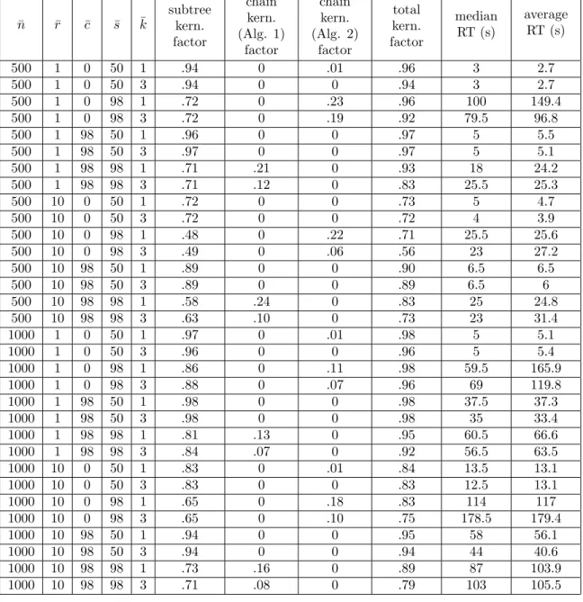
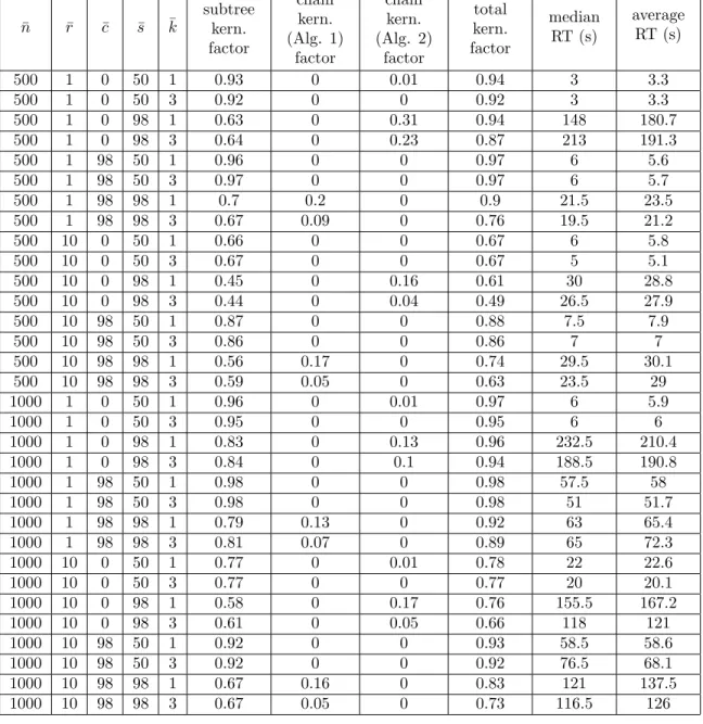
move is where a subtree is detached and regrafted elsewhere in the tree: such moves [10, 21, 27] are often used in experiments to induce increasing hybridization number [1, among others]. Finally, in all but one of the trees a subset of ¯c % of the edges are contracted. The kernelization algorithms are run with k = ¯k. Table 1 shows the results for three trees and Table 2 for four trees. Each row is the average of 10 runs with the given combination of parameters. We give the average kernelization factor – defined as the ratio between the number of leaves removed and the original number of leaves ¯n – as wel as the average and median running times. Our aim is to show that our algorithms are practical, by showing that the kernelization factor is high for several combinations of parameters. Moreover, we also want to test for which combinations of parameters the subtree reduction (Algorithm 1) and chain reductions (Algorithm 1 and 2) are more effective (their kernelization factors are reported in columns 6-8, these are also defined with respect to ¯n so can be summed to obtain the total kernelization factor).
6.2. Analysis of experiments
Given the large number of taxa involved (500 and 1000) it is encouraging to observe that the implementation runs quickly: on a 3.1GHz processor with 4Gb of RAM every parameter combination terminated within 10 minutes, and many parameter combinations were significantly faster, see the last two columns of the tables. Part
¯ n r¯ ¯c s¯ k¯ subtree kern. factor chain kern. (Alg. 1) factor chain kern. (Alg. 2) factor total kern. factor median RT (s) average RT (s) 500 1 0 50 1 .94 0 .01 .96 3 2.7 500 1 0 50 3 .94 0 0 .94 3 2.7 500 1 0 98 1 .72 0 .23 .96 100 149.4 500 1 0 98 3 .72 0 .19 .92 79.5 96.8 500 1 98 50 1 .96 0 0 .97 5 5.5 500 1 98 50 3 .97 0 0 .97 5 5.1 500 1 98 98 1 .71 .21 0 .93 18 24.2 500 1 98 98 3 .71 .12 0 .83 25.5 25.3 500 10 0 50 1 .72 0 0 .73 5 4.7 500 10 0 50 3 .72 0 0 .72 4 3.9 500 10 0 98 1 .48 0 .22 .71 25.5 25.6 500 10 0 98 3 .49 0 .06 .56 23 27.2 500 10 98 50 1 .89 0 0 .90 6.5 6.5 500 10 98 50 3 .89 0 0 .89 6.5 6 500 10 98 98 1 .58 .24 0 .83 25 24.8 500 10 98 98 3 .63 .10 0 .73 23 31.4 1000 1 0 50 1 .97 0 .01 .98 5 5.1 1000 1 0 50 3 .96 0 0 .96 5 5.4 1000 1 0 98 1 .86 0 .11 .98 59.5 165.9 1000 1 0 98 3 .88 0 .07 .96 69 119.8 1000 1 98 50 1 .98 0 0 .98 37.5 37.3 1000 1 98 50 3 .98 0 0 .98 35 33.4 1000 1 98 98 1 .81 .13 0 .95 60.5 66.6 1000 1 98 98 3 .84 .07 0 .92 56.5 63.5 1000 10 0 50 1 .83 0 .01 .84 13.5 13.1 1000 10 0 50 3 .83 0 0 .83 12.5 13.1 1000 10 0 98 1 .65 0 .18 .83 114 117 1000 10 0 98 3 .65 0 .10 .75 178.5 179.4 1000 10 98 50 1 .94 0 0 .95 58 56.1 1000 10 98 50 3 .94 0 0 .94 44 40.6 1000 10 98 98 1 .73 .16 0 .89 87 103.9 1000 10 98 98 3 .71 .08 0 .79 103 105.5
Table 1: Kernelization factors and running times for several combinations of parameters ¯r, ¯c, ¯s, ¯k and ¯n, for ¯t = 3 trees.
¯ n r¯ ¯c s¯ k¯ subtree kern. factor chain kern. (Alg. 1) factor chain kern. (Alg. 2) factor total kern. factor median RT (s) average RT (s) 500 1 0 50 1 0.93 0 0.01 0.94 3 3.3 500 1 0 50 3 0.92 0 0 0.92 3 3.3 500 1 0 98 1 0.63 0 0.31 0.94 148 180.7 500 1 0 98 3 0.64 0 0.23 0.87 213 191.3 500 1 98 50 1 0.96 0 0 0.97 6 5.6 500 1 98 50 3 0.97 0 0 0.97 6 5.7 500 1 98 98 1 0.7 0.2 0 0.9 21.5 23.5 500 1 98 98 3 0.67 0.09 0 0.76 19.5 21.2 500 10 0 50 1 0.66 0 0 0.67 6 5.8 500 10 0 50 3 0.67 0 0 0.67 5 5.1 500 10 0 98 1 0.45 0 0.16 0.61 30 28.8 500 10 0 98 3 0.44 0 0.04 0.49 26.5 27.9 500 10 98 50 1 0.87 0 0 0.88 7.5 7.9 500 10 98 50 3 0.86 0 0 0.86 7 7 500 10 98 98 1 0.56 0.17 0 0.74 29.5 30.1 500 10 98 98 3 0.59 0.05 0 0.63 23.5 29 1000 1 0 50 1 0.96 0 0.01 0.97 6 5.9 1000 1 0 50 3 0.95 0 0 0.95 6 6 1000 1 0 98 1 0.83 0 0.13 0.96 232.5 210.4 1000 1 0 98 3 0.84 0 0.1 0.94 188.5 190.8 1000 1 98 50 1 0.98 0 0 0.98 57.5 58 1000 1 98 50 3 0.98 0 0 0.98 51 51.7 1000 1 98 98 1 0.79 0.13 0 0.92 63 65.4 1000 1 98 98 3 0.81 0.07 0 0.89 65 72.3 1000 10 0 50 1 0.77 0 0.01 0.78 22 22.6 1000 10 0 50 3 0.77 0 0 0.77 20 20.1 1000 10 0 98 1 0.58 0 0.17 0.76 155.5 167.2 1000 10 0 98 3 0.61 0 0.05 0.66 118 121 1000 10 98 50 1 0.92 0 0 0.93 58.5 58.6 1000 10 98 50 3 0.92 0 0 0.92 76.5 68.1 1000 10 98 98 1 0.67 0.16 0 0.83 121 137.5 1000 10 98 98 3 0.67 0.05 0 0.73 116.5 126
Table 2: Kernelization factors and running times for several combinations of parameters ¯r, ¯c, ¯s, ¯k and ¯n, for ¯t = 4 trees.
of the reason for this is the subtree reduction, which is the asymptotically fastest part of the kernelization. The subtree reduction always executes first and this has the effect of significantly reducing the number of taxa before the chain reductions are executed. The kernelization factors of the chain reductions are much smaller, partly because they are calculated relative to the original number of taxa, before the subtree reduction.
Looking at the table more closely, a number of observations can be made. Clearly, in this experimental setup both chain reductions require that the starting tree T1 is
heavily chain-like, which is achieved by having a skew factor close to 100. Otherwise the starting tree T1 is too “bushy” and under the action of rSPR moves no long
chains are formed. Secondly, if there is no contraction, then all the trees are binary, and the degree-based chain reduction (Algorithm 2) has quite a large impact, while Algorithm 1 has no impact at all. If there is an extremely large amount of contraction, then the roles of the two chain reductions are reversed. An intermediate amount of contraction (not shown in the table) effectively disables both chain reductions, but not the subtree reduction. Conversely, a growing number of rSPR moves (which have the effect of increasing the topological dissimilarity of the trees) reduces the impact of the subtree reduction but not of the chain reduction. As k = ¯k increases, the impact of both chain reductions diminishes, due to the increasing of the length at which chains are truncated. However, the impact of the reductions decreases only slightly when k is increased from 1 to 3. This is encouraging, suggesting that both chain reductions can have an impact for larger values of k. Similarly, increasing the number of trees has only a very small negative effect on the impact of the subtree and chain reductions. Finally, as the total kernelization factors in the table show, it is clear that the kernelization “works”: for all parameter combinations in the tables the instances reduce in size by at least 49%.
7. Discussion and open problems
The main open question remains whether the Hybridization Number problem is fixed-parameter tractable, and if it has a polynomial kernel, when parameter-ized only by k (that is, when the number of input trees and their outdegrees are unbounded).
Note that when the input trees are not required to have the same label set X, Hybridization Number is not fixed-parameter tractable unless P = NP. The reason for this is that it is NP-hard to decide if r(T ) = 1 for sets T consisting of trees with three leaves each [16, Theorem 7].
Another question is whether the kernel size can be reduced for certain fixed |T |. For |T | = 2, our results give a cubic kernel, while Linz and Semple [20] showed a linear kernel of a modified, weighted problem, by analyzing carefully how common chains can look in two trees. Can something like this be done for more than two trees? In particular, does there exist a quadratic kernel for three trees? In addition, can the running times of the kernelization algorithms be reduced?
Finally, there is the problem of solving the kernelized instances. For this, a fast exponential-time exact algorithm is needed, or a good heuristic. Although we have presented an O(nf (k)t) time algorithm for Hybridization Number, with n = |X|
and t = |T |, it is not known if there exists an O(cn)-algorithm for some constant c.
While O(cknO(1)) algorithms have been developed for instances consisting of two binary trees [28] and very recently for three binary trees [14], it is not clear if they exist for four or more binary trees, or for two or more nonbinary trees. Note that, for practical applications, the kernelization can also be combined with an efficient heuristic.
Acknowledgements
We thank the anonymous reviewers for their helpful comments.
[1] B. Albrecht, C. Scornavacca, A. Cenci, D.H. Huson, Fast computation of mini-mum hybridization networks, Bioinformatics 28 (2): 191–197, 2012.
[2] E. Bapteste, L. van Iersel, A. Janke, S. Kelchner, S. Kelk, J. O. McInerney, D. A. Morrison, L. Nakhleh, M. Steel, L. Stougie, J. Whitfield, Networks: expanding evolutionary thinking, Trends in Genetics 29 (8): 439 – 441, 2013.
[3] M. Baroni, S. Gr¨unewald, V. Moulton, C. Semple, Bounding the number of hybridisation events for a consistent evolutionary history, Mathematical Biology 51: 171–182, 2005.
[4] H. L. Bodlaender, R. G. Downey, M. R. Fellows, D. Hermelin, On problems without polynomial kernels, Journal of Computer and System Sciences 75 (8): 423–434, 2009.
[5] M. Bordewich, C. Semple, Computing the minimum number of hybridization events for a consistent evolutionary history, Discrete Applied Mathematics 155 (8): 914–928, 2007.
[6] M. Bordewich, C. Semple, Computing the hybridization number of two phylo-genetic trees is fixed-parameter tractable, IEEE/ACM Transactions on Compu-tational Biology and Bioinformatics 4 (3): 458–466, 2007.
[7] Z.-Z. Chen, L. Wang, Algorithms for reticulate networks of multiple phylogenetic trees, IEEE/ACM Transactions on Computational Biology and Bioinformatics 9 (2): 372–384, 2012.
[8] Z.-Z. Chen, L. Wang, An ultrafast tool for minimum reticulate networks, Journal of Computational Biology 20 (1): 38–41, 2013.
[9] R. G. Downey, M. R. Fellows, Parameterized complexity, Springer-Verlag, 1999. [10] J. Hein, Reconstructing evolution of sequences subject to recombination using
parsimony, Mathematical biosciences 98 (2): 185–200, 1990.
[11] D. H. Huson, R. Rupp, C. Scornavacca, Phylogenetic networks: concepts, algo-rithms and applications, Cambridge University Press, 2011.
[12] L. van Iersel, Algorithms, haplotypes and phylogenetic networks, PhD Thesis, 2009.
[13] L. van Iersel, S. Kelk, N. Leki´c, L. Stougie, Approximation algorithms for nonbi-nary agreement forests, SIAM Journal on Discrete Mathematics 28 (1): 49–66, 2014.
[14] L. van Iersel, S. Kelk, N. Leki´c, C. Whidden, N. Zeh, Hybridization number on three trees, ArXiv:1402.2136 [cs.DS], 2014.
[15] L. van Iersel, S. Linz, A quadratic kernel for computing the hybridization number of multiple trees, Information Processing Letters 113 (9): 318 – 323, 2013. [16] J. Jansson, N. B. Nguyen, W.-K. Sung, Algorithms for combining rooted triplets
into a galled phylogenetic network, SIAM Journal on Computing 35 (5): 1098– 1121, 2006.
[17] S. Kelk, L. van Iersel, N. Leki´c, S. Linz, C. Scornavacca, L. Stougie, Cycle killer... qu’est-ce que c’est? On the comparative approximability of hybridization num-ber and directed feedback vertex set, SIAM Journal on Discrete Mathematics 26 (4): 1635–1656, 2012.
[18] S. Kelk, C. Scornavacca, Towards the fixed parameter tractability of con-structing minimal phylogenetic networks from arbitrary sets of nonbinary trees, arXiv:1207.7034 [q-bio.PE], 2012.
[19] S. Kelk, C. Scornavacca, Constructing minimal phylogenetic networks from soft-wired clusters is fixed parameter tractable, Algorithmica 68: 886–915, 2014. [20] S. Linz, C. Semple, Hybridization in non-binary trees, IEEE/ACM Transactions
on Computational Biology and Bioinformatics 6 (1): 30–45, 2009.
[21] W. Maddison, Gene trees in species trees, Systematic biology (3): 523–536, 1997.
[22] C. McDiarmid, C. Semple, D. Welsh, Counting phylogenetic networks, Annals of Combinatorics, 19 (1): 205-224, 2015.
[23] D. Morrison, Introduction to phylogenetic networks, RJR Productions, Uppsala, 2011.
[24] L. Nakhleh, D. Ringe, T. Warnow, Perfect phylogenetic networks: a new methodology for reconstructing the evolutionary history of natural languages, Language 81 (2): 382–420, 2005.
[25] T. Piovesan, S. Kelk, A simple fixed parameter tractable algorithm for comput-ing the hybridization number of two (not necessarily binary) trees, IEEE/ACM Transactions on Computational Biology and Bioinformatics 10 (1): 18–25, 2013. [26] C. Semple, M. Steel, Phylogenetics, Oxford University Press, 2003.
[27] Y.S. Song, J. Hein, Parsimonious reconstruction of sequence evolution and hap-lotyde blocks: finding the minimum number of recombination events, Algorithms in Bioinformatics (WABI 2003) 2812: 287–302, 2003.
[28] C. Whidden, R. G. Beiko, N. Zeh, Fixed-parameter algorithms for maximum agreement forests, SIAM Journal on Computing 42 (4): 1431–1466, 2013. [29] Y. Wu, Close lower and upper bounds for the minimum reticulate network of
multiple phylogenetic trees, Bioinformatics 26: i140–i148, 2010.
[30] Y. Wu, An algorithm for constructing parsimonious hybridization networks with multiple phylogenetic trees, Journal of Computational Biology 20 (10): 792–804, 2013.