HAL Id: cea-02421883
https://hal-cea.archives-ouvertes.fr/cea-02421883
Submitted on 20 Dec 2019
HAL is a multi-disciplinary open access
archive for the deposit and dissemination of
sci-entific research documents, whether they are
pub-lished or not. The documents may come from
teaching and research institutions in France or
abroad, or from public or private research centers.
L’archive ouverte pluridisciplinaire HAL, est
destinée au dépôt et à la diffusion de documents
scientifiques de niveau recherche, publiés ou non,
émanant des établissements d’enseignement et de
recherche français ou étrangers, des laboratoires
publics ou privés.
Covariance matrices of the hydrogen neutron cross
sections bound in light water for the JEFF-3.1.1 neutron
library
G. Noguere, J. Scotta, C. de Saint-Jean, P. Archier
To cite this version:
G. Noguere, J. Scotta, C. de Saint-Jean, P. Archier. Covariance matrices of the hydrogen neutron
cross sections bound in light water for the JEFF-3.1.1 neutron library. Annals of Nuclear Energy,
Elsevier Masson, 2017, 104, pp.132-145. �10.1016/j.anucene.2017.01.044�. �cea-02421883�
Covariance matrices of the hydrogen neutron cross sections
bound in light water for the JEFF-3.1.1 neutron library.
G. Noguere, J.P. Scotta, C. De Saint Jean and P. Archier CEA, DEN, DER Cadarache, F-13108 Saint Paul les Durance, France
Abstract
In the international neutron libraries, the behavior with the energy of the neutron cross sec-tions of hydrogen in light water depends on the thermal scattering laws tabulated in terms of S(α, β). For the Joint Evaluated Fission and Fusion library (JEFF), Mattes and Keinert have established thermal scattering laws by using the LEAPR module of the NJOY code. However, uncertainties on the corresponding S (α, β) were never reported. Such missing information was recently calculated with the nuclear data code CONRAD by determining the covariances between the model parameters involved in LEAPR. The obtained uncertainties were propagated to reac-tivity coefficients calculated for critical assemblies operating in ”cold” conditions (temperature below 80◦C) and for PWR in ”hot” operating conditions (300◦C). For the integral benchmarks
investigated in this work, we found that the uncertainty on the calculated ke f f, due to the S (α, β)
uncertainties, is close to ±130 pcm at room temperature and ±50 pcm at 300◦C.
Keywords: Thermal Scattering Law, Covariance Matrix, Marginalization, Zero-Variance Penalty, CONRAD, LEAPR, NJOY
1. Introduction
The hydrogen neutron cross section bound in light water depends on the Thermal Scatter-ing Laws (TSL) that contain all the dynamic and structural information about the target system. They modify the energy and angular distributions of scattered neutrons by taking into account the intermolecular and intramolecular hydrogen bounds in the water molecule. In the JEFF-3.1.1 library (Santamarina et al., 2009), the TSL for light water were established by Mattes and Keinert (2005) with the LEAPR model of the NJOY code (MacFarlane, 1994). Covariance information on the corresponding dynamic structure factors tabulated in terms of S (α, β) were never pro-duced making impossible a correct propagation of the neutron cross sections uncertainties due to Hydrogen in neutronic calculations.
Previous tentatives for propagating uncertainties due to Hydrogen cross sections with the Total Monte Carlo technique (Koning and Rochman, 2008) are mainly based on random TSL produced by varying the LEAPR parameters assuming they are all independent (Rochman and Koning, 2013; Cabellos et al., 2014). Such approaches applied to critical benchmarks of the ICSBEP database confirm that non negligible effects ranging from few tens to several hundred of pcm can be achieved. A more elaborate Monte-Carlo technique was also proposed by Holmes and Hawari (2014). It consists in generating a S (α, β) covariance matrix by sampling an ab
0,0 0,1 0,2 0,3 0,4 0,5 Vibration energy (eV)
0,0 2,0 4,0 6,0 8,0 10,0 12,0
Frequency spectrum (1/eV)
Streching modes
Bending mode
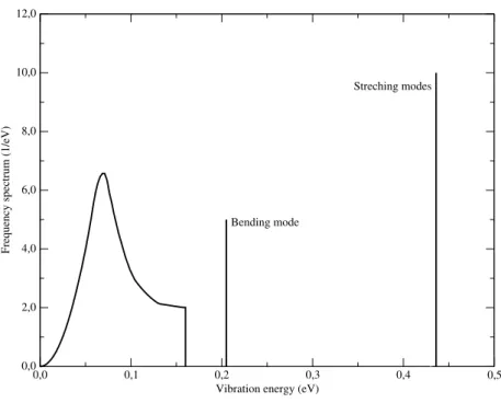
Figure 1: Continuous distribution wcρc(β) and discrete oscillators (E1 = 205 meV, E2 = 436 meV) used in JEFF-3.1.1
at T=294 K. The weights are wc= 0.4891, w1= 0.1630 and w2= 0.3261 respectively.
initiophonon frequency spectrum. In the present work, an analytical method instead of a Monte-Carlo approach is used, in which all the parameters are assumed to be normally distributed. The inaccuracy of the Gaussian assumption has not been quantified in the context of this work. Preliminary results are reported in reference Scotta et al. (2016).
The objective is to determine a S (α, β) covariance matrix associated to the JEFF-3.1.1 library that takes into account the uncertainties not only due to the experimental neutron cross sections but also due to the models implemented in LEAPR. The method relies on the mathematical framework implemented in the CONRAD code (Archier et al., 2014). The uncertainties due to the resulting S (α, β) covariance matrix will be propagated to reactivity coefficients calculated for critical assemblies operating in ”cold” conditions and for PWR in normal operating conditions.
2. Thermal Scattering Laws for H in H2O
The Thermal Scattering Laws for H in H2O available in the JEFF-3.1.1 library were
calcu-lated with the LEAPR module of the NJOY code (Mattes and Keinert, 2005). This module is used to tabulate the asymmetric form of the S (α, β) as a function of the momentum transfer α:
α = E0+ E − 2 √
E0Ecos(θ)
AkBT
, (1)
β = E0− E kBT
, (2)
where E and E0are the incident and secondary neutron energies, kBis the Boltzmann
con-stant, T is the temperature of the material, cos(θ) is the cosine of the scattering angle in the laboratory system and A is the ratio of the mass of the scattering atom to the neutron mass. The double-differential inelastic neutron scattering cross section in the incoherent approximation is then obtained as follows:
∂2σ
∂α∂β =
AkBTσs
4E e
−β/2S(α, β). (3)
in which σsrepresents the free scattering cross section for hydrogen. A detailed description
of the approximations used in LEAPR to calculate the elements of the S (α, β) matrix can be found in reference MacFarlane (1994).
The symmetric S (α, β) dynamic structure factor, as implemented in LEAPR, depends on the frequency spectrum ρ(β) that contains a complete description of the intermolecular and in-tramolecular vibration modes of the water molecule. In LEAPR, ρ(β) has to be split in two parts:
ρ(β) = wtρt(β, c)+ ρs(β). (4)
The first term ρt(β, c) represents the translational component of the water molecule that
de-pends on the diffusion constant c. The second term ρs(β) is decomposed in three components:
ρs(β)= wcρc(β)+ w1δ(βE1)+ w2δ(βE2), (5)
where ρc(β) is a continuous distribution that describes the rotational mode of the water
molecule and w1δ(βE1)+w2δ(βE2) is a sum of two discrete oscillators which define the
intramolec-ular vibrations, namely bending and stretching (Fig. 1). The weights satisfy the following con-straint:
wc+ wt+ w1+ w2= 1. (6)
The structure factors St(α, β) and Ss(α, β) corresponding to each component of Eq. (4) are
then folded as follows:
S(α, β)= St(α, β)e−αλs+
Z +∞
−∞
St(α, β0)Ss(α, β − β0)dβ0, (7)
where λsrepresents the Debye-Waller coefficient:
λs=
Z +∞
−∞
ρ(β)e−β/2
2β sinh(β/2)dβ. (8)
The expression of St(α, β) depends on the value of the diffusion constant c. Mattes et al. use
a diffusion constant c = 0 in order to represent the translational part of ρ(β) with a free gas law. Modern descriptions of the thermal scattering laws of H in H2O indicate that a diffusion constant
cgreater than zero is needed for an accurate description of the neutron cross sections of water. In that case, the Egelstaff and Schofield expression is used (Egelstaff and Schofield, 1962).
10−4 10−3 10−2 10−1 100 101 Energy (eV) 0.0 100.0 200.0 300.0 400.0 500.0 H2
O total cross section (barns)
EXFOR data JEFF−3.1.1
Figure 2: Total neutron cross section of H2O calculated with the Mattes’ parameters at T = 294 K and compared with
experimental data retrieved from the EXFOR database.
The choice of Mattes et al. (c= 0) has an effect on the cross sections in the cold neutron en-ergy range (E < 25.3 meV). Fig. 2 compares the scattering cross section of water calculated with NJOY by using the LEAPR parameters established by Mattes et al. at T = 294 K with experi-mental data retrieved from the EXFOR database. The large discrepancy between the theoretical curve and the data, observed below the thermal neutron energy, can be reduced by increasing the value of the diffusion constant c. Consequences on the determination of the S (α, β) covariance matrix will be discussed in Section 4.
3. Definition of the model parameters
The generation of a S (α, β) covariance matrix requires the determination of the covariance matrix between the model parameters involved in LEAPR. Values of the parameters at 294 K and 574 K are reported in Table 1. The parameters of interests for this work are the weights (wc,
wt, w1 and w2) and the phonon spectrum ρc(β). The diffusion constant c is treated separately
because of c= 0 in the work of Mattes et al. The energies of the discrete oscillators (E1and E2)
also require a specific treatment, their values being well established from previous experimental works and Molecular Dynamic simulations (Marquez Damian et al., 2014). Similarly, the free scattering cross section for hydrogen σs, involved in Eq. (3), is a fixed model parameter whose
value and uncertainty have been reviewed in previous works (Mughaghab, 2006; Carlson et al., 2009; Plompen et al., 2013).
Table 1: LEAPR parameters for H in H2O at 294 K and 574 K established by Mattes and Keinert (2005).
Parameters T=294 K T=574 K
Diffusion constant c 0.0 0.0
Energy interval (meV) δ 2.542 2.542
First oscillator energy (meV) E1 205.0 205.0
Second oscillator energy (meV) E2 436.0 436.0
Continuous spectrum weight wc 0.4891 0.4773
Translational weight wt 0.0217 0.0454
First oscillator weight w1 0.1630 0.1591
Second oscillator weight w2 0.3261 0.3182
Free scattering cross section (barn) σs 20.478 20.478
3.1. Variable parameters
The weights involved in Eqs (4) and (5) are linked by the relationship (6). In this work, we have introduced two factors:
Fwt+ G(wc+ w1+ w2)= 1, (9)
where F is a normalizing multiplicative factor of unity with its own distinct uncertainty and Gis obtained as follow:
G= 1 − Fwt
wc+ w1+ w2
. (10)
The continuous part of the phonon spectrum ρc(β) is a probability density function
normal-ized to unity. The interpretation of ρc(β) as a variable parameter is not straightforward. Figure 3a
shows that the shape of the phonon spectrum in JEFF-3.1.1 is very different from the one ob-tained by Molecular Dynamic simulations (CAB model). In JEFF-3.1.1, the frequency spectra of H in H2O are based on experimental values measured by Page and Haywood at 294 K and
550 K (Page and Haywood, 1968). The experimental spectrum suffers from different sources of uncertainties such as the experimental time resolution which is unknown. In addition, the phonon spectrum introduced in the Mattes’ model is not exactly the original experimental spectrum. The translational part was removed from the experimental spectrum to get a Debye shape in the low vibration energy range. For simplicity, we decided to account for the uncertainty on the phonon spectrum with a scaling factor∆. The latter variable is applied to the vibration energy grid ek
which is used to reconstruct the phonon distribution:
ek= ∆kδ, (11)
in which δ is the energy interval given in the LEAPR input file. This strategy was applied in the US library ENDF/B-VII.1. At room temperature, Fig. 3b shows that the phonon spectrum is simply shifted by a factor∆ ' 0.85. Figure 4 illustrates the impact of ∆ on the calculated total cross section of H2O. A 10% variation of∆ implies an increase of 2% of the thermal cross
section. The weakness of the present approach when large uncertainties are involved is discussed in section 4.5.
The multiplicative and scaling factors (F and∆) are free parameters. The least-squares fitting procedure is shortly explained in Section 4.1.
0.00 0.05 0.10 0.15 0.20 Vibration energy (eV)
0.0 2.0 4.0 6.0 8.0
Frequency spectrum (1/eV)
CAB model JEFF−3.1.1 (∆=1.0) (a)
0.00 0.05 0.10 0.15 0.20
Vibration energy (eV) 0.0
2.0 4.0 6.0 8.0
Frequency spectrum (1/eV)
ENDFB−VII.1 JEFF−3.1.1 (∆=1.0) JEFF−3.1.1 (∆=0.85) (b)
Figure 3: Comparison of the continuous part of the phonon spectrum of H in H2O used in the US library ENDF
/B-VII.1 (MacFarlane, 1994), in the European library JEFF-3.1.1 (Mattes and Keinert, 2005) and calculated by Molecular Dynamic simulations (CAB model) (Marquez Damian et al., 2014) at room temperature.
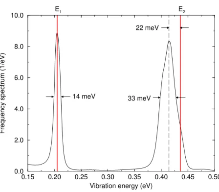
3.2. Energies of the bending and streching modes
In the water molecule, the intramolecular vibrations are related to the bending and streching modes. In the Mattes’ model, these modes are described by two discrete oscillators located at E1 = 205 meV and E2 = 436 meV. As shown in Fig. 5, the energy of the first oscillator is in
good agreement with the mean energy calculated by Molecular Dynamic simulations (Marquez Damian et al., 2014). For the second oscillator, an energy shift of about 22 meV is observed. The water potential introduced in the simulations were optimized with vibration energies measured by Lappi et al. (2004).
The discrete representation does not take into account the spread around the mean value. The calculated Full Widths at Half Maximum are 14 meV and 33 meV respectively, providing uncertainties on the position of the two oscillators close to 6 meV and 14 meV. The uncertainty associated to the streching mode is larger because the symmetric and asymmetric vibrations are merged in a single discrete oscillator.
0 100 200 300 400
Total cross section (barn)
∆=1.0 ∆=1.1 10−4 10−3 10−2 10−1 100 101 Energy (eV) 0.96 0.98 1.00 1.02 1.04 Ratio σt(∆=1.1)/σt(∆=1.0)
Figure 4: Effect on the H2O total cross section of the scaling factor∆ applied to the vibration energy grid used to
reconstruct the phonon distribution at T= 294 K.
Table 2: Free scattering cross section for Hydrogen reported in the literature.
Author Year σs Mughaghab 2006 20.491 ± 0.014 b (0.06%) Carlson et al. 2009 20.431 ± 0.041 b (0.20%) Plompen et al. 2013 20.474 ± 0.012 b (0.06%) mode: E1= 205 ± 6 meV,
while, the uncertainty on E2should account for the calculated width and the energy shift of
22 meV. The addition of the two contributions leads to: E2 = 436 ± 36 meV.
3.3. Free scattering cross section for Hydrogen
In Eq. (3), the free scattering cross section σs is defined as the sum of the coherent and
incoherent scattering cross sections:
σs= σcoh+ σinc. (12)
0.15 0.20 0.25 0.30 0.35 0.40 0.45 0.50 Vibration energy (eV)
0.0 2.0 4.0 6.0 8.0 10.0
Frequency spectrum (1/eV)
22 meV
14 meV 33 meV
E1 E2
Figure 5: Bending and streching modes calculated at T = 294 K with the molecular dynamic code GROMACS and parameters used in reference Marquez Damian et al. (2014). The mean energies of the two modes (205.2 meV and 414.5 meV) are compared with the energies of the first and second oscillators introduced in the Mattes’ model (E1=205 meV
and E2=436 meV).
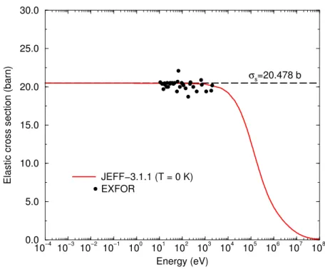
For Hydrogen, the value of σscan be found in the Evaluated Neutron Data Files in
ENDF-6 format. Figure ENDF-6 shows the scattering cross section of Hydrogen at T = 0 K as given in the international library JEFF-3.1.1. Below 1 eV, the cross section is nearly constant and fully compatible with the free scattering cross section of 20.478 barns used by Mattes.
More recent evaluated values were reported in the literature. Table 2 summarizes the most relevant results. The one from Plompen et al. (2013) confirms the free scattering cross section used in the JEFF-3.1.1 library. However, the given uncertainty of ±0.012 barns is too low, be-cause the weighted average was calculated over few experimental results without introducing experimental correlations. In the present work, we decided to follow the relative uncertainty of ±0.2% recommended by the Neutron Standard Working Group of AIEA (Carlson et al., 2009):
σs= 20.478 ± 0.041 barns.
3.4. Diffusion constant
As shown in Fig. 2, the elastic cross section for H in H2O calculated with the LEAPR
param-eters established by Mattes et al. nearly follows the experimental trend in a large energy range of interest for light water reactor applications. Below 1 meV, the calculations fail to correctly reproduce the experimental values. When the model calculations deviate significantly from the
10−4 10−3 10−2 10−1 100 101 102 103 104 105 106 107 108 Energy (eV) 0.0 5.0 10.0 15.0 20.0 25.0 30.0
Elastic cross section (barn) JEFF−3.1.1 (T = 0 K)
EXFOR
σ
s=20.478 b
Figure 6: Hydrogen scattering cross section given in the neutron libraries JEFF-3.1.1 compared to experimental data retrieved from the EXFOR database. The dashed line represents the free scattering cross section σsused in the Mattes’
model.
measurements, Leeb et al. have proposed to account for Model Defects in covariance matri-ces (Neudecker et al., 2013).
The proposed strategies mainly consist to add extra covariance terms for producing large uncertainties that cannot be explained by the model parameters. In the case of the Mattes’ work, the origin of the Model Defects observed in the cold neutron energy range is directly related to the choice of the diffusion constant c = 0. By considering a transmission Tth(E) defined as:
Tth(E)= e−nσt(E), (13)
where
σt(E)= 2σtH(E)+ σtO(E), (14)
instead of a total cross section σt(E) in the least-squares fitting procedure, the diffusion
con-stant acts as a background term that mainly affects the low energy range of the theoretical trans-mission. The magnitude of variation of such a background term can be estimated from values reported in the literature. According to the new LEAPR parametrization established by Marquez Damian et al. (2014), a diffusion constant close to c ' 4 is suitable. Figure 7 shows the impact of the diffusion constant on a theoretical transmission calculated for n = 0.017 atom/barn. As expected, sizeable differences are observed below 1 meV.
10−4 10−3 10−2 10−1 100 101 Energy (eV) 0.60 0.80 1.00 1.20 1.40 Ratio Tth(c=4.0)/Tth(c=0.0) 10−3 10−2 10−1 100 Transmission 0.00 0.20 0.40 0.60 Transmission Tth(c=0.0) Tth(c=4.0)
Figure 7: Modifications of the low energy part of a given theoretical transmission of a thick water sample according to the diffusion constant c. The areal density used in the calculation is n = 0.017 atom/barn.
3.5. Experimental parameters
For the correct determination of the covariance matrix between the LEAPR parameters, we also need to include experimental uncertainties. In practice, long range correlations are taken into account by introducing in the calculation of the transmission coefficient (Eq. (13)) a normal-ization factor N and a background correction B:
T(E)= NTth(E)+ B, (15)
In the present work, no background correction is taken into account. As shown in Fig. 7, the diffusion constant c should encompass such a contribution. For most of the H2O total cross
section reported in the EXFOR database, the uncertainty on the normalization factor is poorly documented. Owing to the accuracy of the transmission measurements achieved over the last ten years in the existing time-of-flight facilities, a 1% uncertainty was considered in our calculations:
∆N = 0.01
The uncertainty on the temperature T was also considered. Unfortunately, the accuracy of this experimental parameter is also poorly documented and no information is reported in the EXFOR database. From room (T = 294 K) to high (T = 574 K) temperature conditions, we decided to use an uncertainty of 2 K:
The uncertainty of the normalization and of the temperature is included in the uncertainty propagation procedure by ”marginalization”. The technique is explained in section 4.2.
4. Covariance matrix between the LEAPR parameters
The analytical method applied to generate the covariance matrix between the LEAPR param-eters relies on the least-squares fitting procedure of the CONRAD code (Archier et al., 2014), in which mathematical algorithms were implemented to account for uncertainties of various origins. Each step of the CONRAD calculation is described below and illustrated with results obtained at T = 294 K. Results obtained at T = 294 K and T = 574 K are compared and discussed in section 4.5.
4.1. Retroactive analysis
The objective of the present work is to provide a covariance matrix between the LEAPR parameters, without changing the value of the parameters. The ”retroactive” approach is a method designed to generate uncertainties for existing model parameters by taking into account all sources of experimental uncertainties (Habert et al., 2010). It is based on the use of theoretical cross sections to simulate various experiments. Statistical uncertainties and systematic uncertain-ties, such as normalization, are then added to these theoretical values rendering them as close as possible to a true experiment. The principle of ”retrofitting” pre-existing evaluations that did not originally provide covariances is not as rigorous as a new evaluation work. This issue was addressed by Smith (2011). However, no other analytical method was proposed for providing usable covariances between existing model parameters. The origin of the uncertainties are given in section 3 and the different operations are described below for ensuring the traceability of our uncertainty propagation work.
The observable parameters of interest are defined in section 3.1. They are all assumed to be normally distributed. The impact of this assumption on the final covariances has not been investigated. Let ~x = (∆, F)T the vector that contains the scaling and multiplicative factors, and Mx the corresponding covariance matrix. At the beginning of the fitting procedure, we
assume that the parameters are poorly known and independent, making the prior covariance matrix diagonal with uninformative prior variances. In practice, the relative prior uncertainties for∆ and F are set to 10%. At the end of the retroactive fitting procedure, the central values of the parameters are unchanged, but the obtained uncertainties are rather low:
∆ = 1.000 ± 0.005, F= 1.000 ± 0.013.
They only take into account the contribution of the uncorrelated uncertainties taken from the EXFOR database. Contributions due to other sources of uncertainties are included by using a marginalization procedure.
4.2. Marginalization procedure
The marginalization procedure was first developed in the CONRAD code to propagate ex-perimental uncertainties (De Saint Jean et al., 2009). The procedure was then generalized to account for experimental and model parameters with known uncertainties through the Zero Vari-ance Penalty algorithm. Main results reported in reference Noguere et al. (2012) are summarized below.
The Zero Variance Penalty algorithm consists in dividing the model parameter sequence in two blocks of variables.
~µ = ~θ~x !, (16)
where ~xcontains the observable variables, as defined in section 4.1, and ~θ contains ”latent” and ”nuisance” variables. Latent variables (as opposed to observable variables) may define re-dundant parameters or hidden variables that cannot be observed directly. This term reflects the fact that such variables are really there, but they cannot be observed or measured for practical reasons. Nuisance variables correspond to aspect of physical realities whose properties are not of particular interest as such but are fundamental for assessing reliable model parameters. In the present work, the nuisance parameters are the normalization N and the temperature T . The latent parameters are the free scattering cross section σsand the energies of the discrete oscillators E1
and E2. The contribution of the diffusion constant c is treated independently, as this
parame-ter is related to a Model Defect. The covariance matrix between the model parameparame-ters can be partitioned as follow:
Σ = Σ11 Σ12
Σ21 Σ22
!
. (17)
Each element of the covariance matrixΣ is given by: Σ11 = Mx+ (GTxGx)−1GTxGθMθGTθGx(GTxGx)−1, Σ12 = −(GTxGx)−1GTxGθMθ, Σ22 = Mθ, (18)
where Mx stands for the covariance matrix between the best-fit values of the observable
variables and Mθrepresents the covariance matrix between the latent and nuisance parameters. In the present work, the covariance matrix Mxaccounts for the uncorrelated uncertainties coming
from the experimental total cross sections, while the second term ofΣ11accounts for systematic
uncertainties that create long range correlations between the experimental data.
For a vector quantity ~z of general dimension k, the derivative matrices Gx and Gθ of the
quantity z to the model parameters x and θ are defined as:
Gx= ∂z1 ∂∆ ∂z∂F1 .. . ... ∂zk ∂∆ ∂z∂Fk , (19) and Gθ= ∂z1 ∂σs ∂z1 ∂E1 ∂z1 ∂E2 ∂z1 ∂N ∂z∂T1 .. . ... ... ... ... ∂zk ∂σs ∂zk ∂E1 ∂zk ∂E2 ∂zk ∂N ∂z∂Tk . (20)
Equations (18) are applied after the fitting procedure. The uncertainties on the observable parameters increase significantly:
0.01 0.02 0.03 0.04 Energy (eV) 80.0 100.0 120.0 140.0 160.0 H2
O total cross section (barns)
EXFOR data JEFF−3.1.1
E=25.3 meV
Figure 8: Comparison of the theoretical and experimental total cross sections of H2O in the thermal energy range at
T= 294 K. The shadow area represents the 1σ uncertainty band obtained by introducing in the calculations a constraint on the thermal cross section.
F= 1.000 ± 0.186. 4.3. Constraint on the thermal cross section
At room temperature, the Mattes’ model overestimates the thermal scattering cross section of H2O. The differences between the theoretical curve and the EXFOR data (Fig. (8)) range
between 5% to 6%. The LEAPR parameters were optimized by Mattes et al. in order to find an agreement as good as possible with the data. Due to the treatment of the translational part and of the shape of the experimental phonon spectrum, it was not possible to accurately reproduce the data. Recently, Marquez Damian et al. (2014) has found a better set of LEAPR parameters in excellent agreement with the data, showing that the LEPAR model is adequate for light water when improved translational contribution and phonon spectrum are used.
An additional normalization term is introduced in the calculations for generating uncertain-ties around the thermal energy consistent with the observed bias. As a result, the uncertainty on the scaling factor∆ increases up to 0.24:
∆ = 1.00 ± 0.24,
and the relative uncertainty on the thermal total cross section of H2O at T = 294 K reaches
5%:
σt= 112.9 ± 5.7 barns.
Table 3: Values, uncertainties and correlations between the LEAPR parameters calculated with the CONRAD code at T= 294 K.
Parameters Values Rel. unc. Correlation matrix
∆ 1.000 ± 0.241 (24.1%) 100.0 σs 20.478 ± 0.041 (0.2%) -1.2 100.0 F 1.000 ± 0.186 (18.6%) 15.3 14.2 100.0 E1 205.0 ± 6.0 (2.9%) -1.2 0.0 6.0 100.0 E2 436.0 ± 36.0 (8.3%) 2.3 0.0 45.7 0.0 100.0 c 0.0 ± 1.5 - 0.0 0.0 0.0 0.0 0.0 100.0
Table 4: Values, uncertainties and correlations between the LEAPR parameters calculated with the CONRAD code at T= 574 K.
Parameters Values Rel. unc. Correlation matrix
∆ 1.000 ± 0.569 (56.9%) 100.0 σs 20.478 ± 0.041 (0.2%) -0.7 100.0 F 1.000 ± 0.093 (9.3%) 8.3 14.6 100.0 E1 205.0 ± 6.0 (2.9%) -0.7 0.0 5.3 100.0 E2 436.0 ± 36.0 (8.3%) 0.5 0.0 45.1 0.0 100.0 c 0.0 ± 1.5 - 0.0 0.0 0.0 0.0 0.0 100.0
Figure 8 compares the theoretical and experimental total cross sections of H2O in the thermal
energy range. The obtained 1σ uncertainty band remains within the upper limit of the experi-mental data.
4.4. Contribution of the diffusion constant
The diffusion constant c is a dimensionless parameter involved in the translational vibration component of the water molecule. In the work of Mattes et al., the diffusion constant is set to zero in order to represent the translational part with a free gas law. A non-zero diffusion constant implies to switch to the Egelstaff and Schofiled expression. As a consequence, c is a parameter that can be easily used to account for Model Defects in the covariance matrix.
The value of the diffusion constant depends on the phonon spectrum introduced in the calcu-lations. In the latest LEAPR model (Marquez Damian et al., 2014), its value reaches c ' 4. For the Mattes’ model, lower amplitude of variation was established by trial and error. We found that the optimal interval of variation for the diffusion constant is close to ±1.5.
The correlation matrix between the LEAPR parameters at T = 294 K is reported in Table 3. Figure 9 shows the relative uncertainties and the correlation matrix obtained for the total cross section of H in H2O with and without the contribution of the diffusion constant. Its sizeable
impact is clearly seen below 10 meV. 4.5. Discussion of the results
The sections 4.1 to 4.4 describe the sequence of operations followed in the present work for calculating covariances between the LEAPR parameters of the Mattes’ model. Each step
(a) T = 294 K
(b) T = 574 K
Figure 9: Relative uncertainties and correlation matrix for the total cross section of H in H2O at 294 K and 574 K without
(left hand plots) and with (right hand plots) the contribution of the diffusion constant c. 15
is illustrated with results obtained at room temperature. The same sequence of operations was repeated at T = 574 K. Values, uncertainties and correlations between the LEAPR parameters are reported in Table 4. The top and bottom plots of Fig. 9 indicate that the structures of the correlation matrix at room temperature and 574 K are nearly similar. The relative uncertainties are also of similar amplitude. For the thermal total cross section of H2O, the relative uncertainty
is close to 8%:
σt= 116.3 ± 9.1 barns.
One of the relevant results is the uncertainty on the scaling factor∆ (Eq. (11)) that ranges from ±0.24 to ±0.57. At room temperature, the obtained uncertainty is consistent with the shift of 0.85 observed between the phonon spectrum used in the JEFF-3.1.1 and ENDF/B-VII.1 libraries (Fig. 3b). Our simplified uncertainty propagation strategy applied to the phonon spectrum pro-vides consistent results when the theoretical calculations are in reasonable agreement with the experimental values. Such a strategy is difficult to apply when the differences between the the-oretical and experimental values become sizeable. In hot conditions, the large uncertainty of ±0.57 is more related to the inaccurate shape of the phonon spectrum used in the LEAPR model of the JEFF-3.1.1 library, rather than to experimental uncertainties.
5. Propagation of the LEAPR parameter uncertainties to S(α, β) 5.1. Dynamic structure factor
As indicated in the Introduction, the main objective of the CONRAD calculations was to provide uncertainties on the dynamic structure factor tabulated in terms of S (α, β). Figure 10 shows the symmetric S (α, β0) for several β0values at T = 294 K. The curves were obtained from
the asymmetric scattering laws provided by the LEAPR code times exp(β0/2). The 1σ
uncer-tainty bands were calculated with the uncertainties and the correlation matrix of Table 3. The uncertainty on the top of the distributions reaches 3%. The corresponding correlation matrices are presented in Fig. 11 for β0ranging from 8.98 to 121.0. Their structures are simple. They are
composed of two correlated blocks, that smoothly change with β0.
5.2. Double differential scattering cross section
Double differential scattering cross sections were not considered for determining the covari-ance matrix between the LEAPR parameters reported in Table 3. The few data sets available in the literature represent valuable experimental information for the validation of the covariances between the S (α, β).
Figure 12 compares the theory to the double differential cross sections measured by Bischoff et al. (1967) at the Linac facility of the Rensselaer Polytechnic Institute (RPI) from E= 0.154 eV to E = 0.631 eV at θ = 25◦. The theoretical curves are broadened assuming that the resolution
function has a Gaussian shape. The width of the Gaussian distribution is a free parameter. The energy resolution∆E/E varies from 1% to 5% according to the angle of the outgoing particle and the incident neutron energy.
The differences between the theory and the data confirm that the Mattes’ model fails to ac-curately reproduce the low amplitude structures due to hindered rotation around the quasi-elastic scattering peak. The covariance matrix reported in Table 3 provides large uncertainty bands, which are consistent with the observed discrepancies.
0.0 50.0 100.0 150.0 200.0 250.0 Momentum tranfert α 0.00 0.01 0.02 0.03 0.04 0.05 Symmetric S( α ,β ) β0=0.0 β0=8.98 β0=31.5 β0=79.8 β0=121.0 β0=158.1
Figure 10: Symmetric S (α, β0) for several β0values at T= 294 K. The solid line are the results of the Mattes’work. The
grey zones are the 1σ uncertainty bands calculated with the uncertainties and the correlation matrix of Table 3.
6. Propagation of the LEAPR parameter uncertainties to integral calculations
A direct perturbation of the LEAPR parameters was used for the propagation of the uncer-tainties reported in Table 3. The method was first investigated on a simple benchmark, namely PST-001.1, of the ICSBEP database, and then applied to UOX core configurations in ”cold” and ”hot” conditions.
6.1. Comparison of the propagation techniques
As already indicated in section 4.1, the techniques chosen in this work for propagating or producing covariances rely on analytic methods in which the variables are Gaussian distributed. In practice, only the two first moments of the distributions are considered. Such a treatment is well adapted to direct perturbations of the model parameters. The inaccuracy of the Gaussian assumption has not been quantified in the context of this work.
A direct perturbation consists in calculating the sensitivity of the calculated ke f f to the
LEAPR parameters by changing the parameter values by ±1%. If such an approach is linked to a Monte-Carlo code, results will depend on the convergence criteria. Impacts of these criteria were studied on a thermal solution of Plutonium taken from the ICSBEP database. We have used the benchmark PST-001.1, for which the Average Neutron Lethargy Causing Fission is close to 0.09 eV. The reactivity calculated with the JEFF-3.1.1 library and the TRIPOLI4 R
code (Both et al., 2003) is ke f f = 1.00140(2).
(a) β0= 8.98 (b) β0= 31.15
(c) β0= 79.8 (d) β0= 121.0
Figure 11: Correlation matrices of the symmetric S (α, β0) for increasing values of β0.
Table 5 reports the results obtained with the TRIPOLI4R code for three convergence criteria.
The two first criteria are low and very close (1.5 pcm and 2.0 pcm). The difference of 1 pcm con-firms the repeatability and reproducibility of our direct calculations. By contrast, the difference increases rapidly (19 pcm) when a convergence of 7 pcm is imposed.
Similar differences are obtained by using the Total Monte-Carlo perturbation method (Kon-ing and Rochman, 2008), for which 1000 random TSL files were generated from the Cholesky decomposition of the covariance matrix between the LEAPR parameters (Table 6). Differences obtained with the SERPENT (Leppanen, 2015) and MCNPR
(Sweezy et al., 2005) codes are nearly equivalent and equal to 12 pcm and 15 pcm, respectively.
These results confirm that methods based on a direct perturbation of the model parameters require severe convergence criteria. For more complex core configurations, the uncertainty asso-ciated to the direct perturbation method could make difficult the accurate quantification of small impacts due to the Thermal Scattering Laws. In that case, more precise calculations of the sen-sitivity coefficients are needed. The new perturbation method implemented in the TRIPOLI4 R
0.03 0.08 0.13 0.18 Energy (eV) 10−1 100 101 102 d 2σ /d Ω dE (arbitrary unit) E=154 meV, θ=25o 0.03 0.08 0.13 0.18 0.23 0.28 Energy (eV) 10−1 100 101 102 d 2σ /d Ω dE (arbitrary unit) E=231 meV, θ=25o 0.03 0.08 0.13 0.18 0.23 0.28 0.33 0.38 0.43 0.48 0.53 0.58 Energy (eV) 10−1 100 101 102 d 2σ /d Ω dE (arbitrary unit) E=499 meV, θ=25o 0.07 0.17 0.27 0.37 0.47 0.57 0.67 0.77 Energy (eV) 10−1 100 101 102 d 2σ /d Ω dE (arbitrary unit) E=631 meV, θ=25o
Figure 12: Double differential scattering cross sections for light water calculated with the Mattes’ model and compared with data measured by Bischoff et al. (1967) at the RPI facility. The grey areas represent the 1σ uncertainty bands calculated with the parameters reported in Table 3.
code based on the Iterative Fission Probability (IFP) could offer suitable alternatives (Truchet et al., 2015).
6.2. Sensibility studies
The direct perturbation of the LEAPR parameters allows to investigate the sensibility of the calculated ke f f to each parameter. Results are summarized in Table 7. When all the LEAPR
pa-rameters are considered, the final uncertainty on the calculated ke f f of the PST-001.1 benchmark
is close to 245 pcm:
ke f f = 1.00140 ± 0.00245.
The decomposition of each contribution shows that the parameters defining the intra-molecular vibrations (E1and E2), the translational mode (c) and the free scattering cross section of
Hydro-gen (σs) have negligible contributions. The scaling factor∆ is the most sensitive parameter and,
in a lesser extent, the multiplicative factor F. 19
Table 5: Differences between the uncertainties on the calculated ke f f for the PST-001.1 benchmark of the ICSBEP
database obtained with the Monte-Carlo code TRIPOLI4 R
. Results have been obtained by a direct perturbation of the LEAPR parameters.
Test Convergence Calculated differences
case criteria ∆ki=1 e f f−∆k i e f f i= 1 1.5 pcm -i= 2 2.0 pcm -1 pcm i= 3 7.0 pcm +19 pcm
Table 6: Differences between the uncertainties on the calculated ke f f for the PST-001.1 benchmark of the ICSBEP
database obtained with the TRIPOLI4 R, SERPENT and MCNPR codes.
Test Monte-Carlo Uncertainty propagation Calculated differences
case code method ∆ki=1
e f f −∆k
i e f f
i= 1 TRIPOLI4 R
Direct perturbation
-i= 2 SERPENT Total Monte-Carlo +12 pcm
i= 3 MCNPR
Total Monte-Carlo +15 pcm
Table 7: Sensitivity studies on the calculated uncertainties∆ke f ffor the PST-001.1 benchmark of the ICSBEP database. Test case LEAPR parameters ∆kie f f ∆kie f f=1−∆ke f fi
i= 1 ∆, F, σs, E1, E2, c ±244.6 pcm
-i= 2 ∆, F, σs, E1, E2 ±244.4 pcm -0.2 pcm
i= 3 ∆, F, σs ±240.6 pcm -4.0 pcm
i= 4 ∆, F ±240.4 pcm -4.2 pcm
i= 5 ∆ ±231.7 pcm -12.9 pcm
The importance of these two parameters is related to their relative uncertainties of 24.1% and 18.6%. The large uncertainty on∆ is due to the differences between the theoretical and experimental total cross sections of light water in the thermal energy range. Any improved descriptions of the phonon spectrum will provide better cross sections around 25.3 meV and will significantly reduce the contribution of∆.
6.3. From room temperature to hot operating conditions
Direct calculations have been performed on more complex UOX core configurations to cover a large temperature range from 6◦C (280 K) to 300◦C (574 K). The uncertainties of the two most sensitive LEAPR parameters (∆ and F) were propagated to the calculated ke f f. For the cold
conditions, we have used the uncertainties and the correlations determined at 294 K (Table 3): ∆ = 1.00 ± 0.24,
F= 1.000 ± 0.186, cor(∆, F) = 0.153.
250 300 350 400 450 500 550 600 Temperature (K) 0 20 40 60 80 100 120 140 160 180 200
Uncertainties on the calculated k
eff
(in pcm)
MISTRAL−1
Hot Zero Power Condition
Figure 13: Uncertainties on the calculated ke f fdue to the LEAPR parameter uncertainties, which were propagated with
the CONRAD code by using TRIPOLI4 R
results. Two different integral benchmarks have been studied. A description of the critical experiment MISTRAL-1 can be found in references Cathalau et al. (1998). In hot conditions, the reported result is associated to a PWR benchmark representative of an UOX core. The quoted uncertainties account for the convergence criteria imposed in the Monte-Carlo calculations, which are 7 pcm and 2.5 pcm, respectively.
∆ = 1.00 ± 0.57, F= 1.000 ± 0.093,
cor(∆, F) = 0.083.
The MISTRAL-1 program, carried out in the EOLE facility of the CEA Cadarache, is a critical experiment designed to investigate the ke f f uncertainties in cold operating conditions at
atmospheric pressure. The residual reactivity was measured as a function of the temperature, from 280 K to 354 K (Cathalau et al., 1998). The comparison between the calculated and the experimental reactivities provides a calculated error on the Reactivity Temperature Coefficient αiso, which is defined as:
∆αiso= ∆
∂ρ ∂T !
. (21)
The Hot Zero Power conditions (574 K, 150 bars) were investigated with a PWR benchmark representative of an Uranium oxide core.
Uncertainties calculated with the CONRAD code by using the TRIPOLI4 R results are
re-ported in Fig. 13. For the MISTRAL-1 configurations, below 354 K, the uncertainty on the 21
Figure 14: Distribution of the error on the Reactivity Temperature Coefficient due to the LEAPR parameter uncertainties calculated ke f f ranges from 125 ± 18 pcm to 137 ± 18 pcm. Around 574 K, a lower uncertainty
close to 54 ± 8 pcm is achieved. The quoted uncertainties account for the convergence crite-ria imposed in the Monte-Carlo calculations. The sensitivity of the calculated ke f f to the TSL
of light water is higher for the MISTRAL-1 configurations because of the contribution of the water reflector of the EOLE reactor. In contrast, our calculations clearly show that, for PWR conditions, the TSL of light water are not the dominant contribution to the uncertainty on the calculated ke f f.
The error on the RTC calculated with the JEFF-3.1.1 library was also investigated with the MISTRAL-1 results (Scotta et al., 2016a). The uncertainty due to the LEAPR parameters were calculated over the temperature range [284 K-354 K]. A propagation of the uncertainties by Monte-Carlo was applied to the TRIPOLI4 R results. The distribution of the error on the RTC
due to the LEAPR parameter uncertainties is shown in Fig. 14. The first and second moments of the distribution provide the following result:
∆αiso= −0.36 ± 0.31 pcm/K.
H2O is rather low compared to other nuclear data. In MISTRAL-1, the dominant contribution is
linked to the thermal shape of the235U neutron cross sections, whose impact can reach 1 pcm/K.
As a consequence, an improved description of the phonon spectrum will have a slight effect on ∆αiso. Such an effect has been studied by Scotta et al. (2016b).
7. Conclusions
An analytical method is described for producing a covariance matrix between the LEAPR parameters involved in the description of the neutron cross sections of H in H2O. The method is
applied to the Mattes’ model used in the JEFF-3.1.1 neutron library. Uncertainties on the LEAPR parameters were propagated by direct perturbation to UOX benchmarks. At room temperature, the uncertainty on the ke f f is close to 130 pcm. In hot conditions, the expected uncertainty is
lower than 100 pcm. Improved perturbation algorithms, such as the IFP in the TRIPOLI4R code,
are needed to quantify small impacts of the Thermal Scattering Laws.
The sensitivities of the calculated ke f f to the LEAPR parameters demonstrate that the final
uncertainties due to the Thermal Scattering Laws are mainly defined by the shape of the continu-ous part of the phonon spectrum. In the present work, it is taken into account by a scaling factor ∆. Any improved description of the phonon spectrum will reduce the uncertainty on ∆, and will lead to lower ke f f uncertainties. For UOX core configurations, the main constraint seems to be
the accurate description of the experimental total cross sections of light water measured at the thermal energy (25.3 meV).
Acknowledgements
Thanks are addressed to Yannick Peneliau, David Bernard and Vincent Pascal for providing TRIPOLI4 Rinputs. The authors also express our gratitude to Dimitri Rochman and Olivier Leray
from the Paul Scherrer Institute for sharing their results obtained with the MCNP Rand SERPENT
codes. We also thank Ignacio Marquez Damian (CNEA, Argentina) for his advices during the preparation of this work, and Oscar Cabello (NEA Data Bank, Paris) for his continuous support.
Archier, P. at al., CONRAD Evaluation Code: Development Status and Perspectives, Nucl. Data Sheets 118, 488 (2014). Bischoff, F. et al., Low Energy Neutron Inelastic Scattering, Rensselaer Polytechnic Institute report, RPI-328-87, 1967. Both, J-P., Tripoli-4 - A three dimensional polykinetic particle transport Monte Carlo code., in Proc. Int. Conf. onR
Supercomputing in Nuclear Applications, SNA2003, Paris, France, 2003. Cabellos, O. et al., Nucl. Eng. Techn. 46, 299 (2014).
Cathalau, S. et al., First validation of neutronic lattice parameters of over-moderated 100% MOX fuelled PWR cores on the basis of the MISTRAL experiment, in Proc. Int. Conf. on the Physics of Nuclear Science and Technology, Long Island, USA, 1998.
Carlson, A.D. et al., Nucl. Data Sheets 110, 3215 (2009) De Saint Jean, C. et al., Nucl. Sci. Eng. 161, 363 (2009). Egelstaff, P.A. and Schofield, P., Nucl. Sci. Eng. 12, 260 (1962). Habert, B. et al., Nucl. Sci. Eng. 166, 276 (2010).
Holmes, J.C. and Hawari, A.I., Nucl. Data Sheets 118, 392 (2014). Koning, A.J and Rochman, D., Ann. Nucl. Ener. 35, 2024 (2008). Lappi, S.E. et al., Spectrochimica Acta Part A 60, 2611 (2004).
Leppanen, J., Serpent - a Continuous-energy Monte Carlo Reactor Physics Burn up Calculation Code, VTT Technical Research Centre of Finland, 2015.
MacFarlane, R.E., New thermal neutron scattering files for ENDF/B-VI, Los Alamos National Laboratory Report, 1994. Mattes, M. and Keinert, J., Thermal neutron scattering data for the moderator materials in ENDF-6 format and as ACE
library for MCNP Rcodes, International Atomic Energy Agency Report, INDC(NDS)-0470, 2005.
Marquez Damian, J.I. et al., Ann. Nucl. Energy 65, 280 (2014).
Mughabghab, S.F. Atlas of Neutron Resonances, 5thedition (Elsevier, Amsterdam, 2006).
Neudecker, D. et al., Nucl. Inst. Meth. A 723, 163 (2013). Noguere, G. et al., Nucl. Sci. Eng. 172, 164 (2012).
Page, D.I. and Haywood, B.C., The Harwell scattering law program: frequency distributions of moderators, Harwell Laboratory Report, AERE-R-5778, 1968.
Plompen, A.J. et al., The status of low energy data for deuterium, oxygen and hydrogen, OECD/NEA Data Bank, JEFDOC-1488, 2013.
Truchet, G. et al., Ann. Nucl. Energy 85, 17 (2015).
Santamarina, A. et al., “The JEFF-3.1.1 Nuclear Data Library”, Technical document, JEFF report 22, 2009. Smith, D., J. Korean Phys. Soc. 59, 755 (2011).
Rochman, D. and Koning, A.J., Nucl. Sci. Eng. 172, 287 (2012). Scotta, J.P. et al., EPJ Web of Conferences 111, 04001 (2016).
Scotta, J.P. et al., Study of neutron scattering in light water in Mistral experiments carried out in EOLE reactor at CEA Cadarache, in Proc. Int. Conf. PHYSOR 2016, Sun Valley, Idaho, USA, 2016.
Scotta, J.P. et al., EPJ Nuclear Sci. Technol. 2, 28 (2016)
Sweezy, J. et al., 2005. MCNP a General Monte Carlo N-Particle Transport Code. Los Alamos National Laboratory, online documentation ”http://mcnp-green.lanl.gov/”.