HAL Id: hal-00714785
https://hal.inria.fr/hal-00714785
Submitted on 5 Jul 2012
HAL is a multi-disciplinary open access
archive for the deposit and dissemination of
sci-entific research documents, whether they are
pub-lished or not. The documents may come from
teaching and research institutions in France or
abroad, or from public or private research centers.
L’archive ouverte pluridisciplinaire HAL, est
destinée au dépôt et à la diffusion de documents
scientifiques de niveau recherche, publiés ou non,
émanant des établissements d’enseignement et de
recherche français ou étrangers, des laboratoires
publics ou privés.
Interactive Computation and Visualization Towards a
Virtual Wind Tunnel
Jérémie Labroquère, Régis Duvigneau, Thibaud Kloczko, Julien Wintz
To cite this version:
Jérémie Labroquère, Régis Duvigneau, Thibaud Kloczko, Julien Wintz. Interactive Computation and
Visualization Towards a Virtual Wind Tunnel. 47th International Symposium of Applied
Aerodynam-ics, Mar 2012, Paris, France. �hal-00714785�
INTERACTIVE COMPUTATION AND VISUALIZATION
TOWARDS A VIRTUAL WIND TUNNEL
J. Labroqu `ere(1), R. Duvigneau(1), T. Kloczko(2)& J. Wintz(2)
INRIA Sophia-Antipolis M ´editerann ´ee, 2004 toute des lucioles, 06902 Sophia-Antipolis, France
(1)OPALE Project-Team, [email protected], [email protected] (2)Experimentation and Development Team, [email protected], [email protected]
INTRODUCTION
Computational Fluid Dynamics (CFD) software is now commonly used for aerodynamic studies as a replacement of traditional experimental facili-ties. CFD codes take benefit from the increase of the computational facilities and the maturity of nu-merical methods. However, they are usually based on old-fashioned software architectures, inherited from the 80s. They are typically built as static codes, independently from software components that are used to construct the geometry and the grid, or visualize flow fields. As a consequence, the whole simulation process is usually quite com-plex, including several different phases, and is re-stricted to expert users. Moreover, it is not possi-ble for the user to interact with the computed flow, which makes a significant difference with an ex-perimental wind tunnel. In the latter case, the user can for instance adjust inflow parameters, or mod-ify some geometrical characteristics such as wing incidence, while interactively observing the flow evolution. The studies on interactive CFD simu-lation are quite uncommon, and a very few papers can be found on this topic [6, 7, 10].
In this study, we investigate the use of a modern software architecture in the context of CFD, which allows the user to interact with the computation, by modifying physical or numerical parameters dur-ing the computation and visualize the impact on the flow. Our objective is to evaluate the interest of such a software architecture and measure the possible benefit for scientific studies.
We describe in a first section the proposed soft-ware architecture and its new features, that allow the user to interact with the computation and vi-sualization. Then, the application to compress-ible flow simulation is considered. In particular, we show that various implementations can be en-visaged, with different advantages and drawbacks. The possible interactions with the computation and visualization are described. In a third section, some illustrations are proposed. Finally, the
bene-fit of the use of these new features are discussed from the point of view of the CFD practitioner.
1. SOFTWARE ARCHITECTURE 1.1 Platform and plugins system
Traditionally, CFD codes are only composed of a main program built with some static libraries. The main program describes more or less the work-flow that corresponds to the simulation, whereas the librairies contain the functions necessary for each task of the workflow. This straightforward program architecture has been set up during the 70s and 80s and has not really be questioned so far, although the complexity of the computations has grown significantly.
However, it appears clearly that this architecture has several drawbacks. First, the achievement of numerical experiments requires modularity, which allows to easily test different numerical methods (e.g. Roe flux v.s. HLLC flux), or modify physical parameters (e.g. inlet velocity profile). This ability to change some parts of the code is critical to pre-cisely benchmark numerical methods or models. Obviously, the traditional static architecture is not well suited to this purpose: usually, the implemen-tation of a new method foo2 yields the addition of new functions and variables, that will juxtapose the existing ones foo0, foo1. Then, the code is always growing and becoming less and less readable.
Developments in CFD are now mainly collabo-rative projects, because it is more and more dif-ficult for one isolated person to master all model-ing, numerical and computational aspects related to complex simulations. Unfortunately, the tradi-tional architecture is a real burden for collaborative development: since these codes are always grow-ing (as explained above), the exchange of pieces of code and the maintenance is time consuming for long term and large scale projects. Typically, for each new method foo2, someone should verify if the proposed implementation is correct and will not generate conflicts with all other existing meth-ods foo0, foo1 (for instance in case of addition of an argument).
Finally, the complexity of these codes make the introduction of a new user tedious and time con-suming: to modify a unique method, a new user should usually understand a large part of the code, even if it is not of interest for his study.
To overcome these limitations, we have initiated the NUM3SIS project (http://num3sis.inria. fr), whose software architecture is based on the distinction between the platform and plugins. The platform, written in C++ language, gathers all com-ponents dedicated to numerical simulation, that are considered as common to various computa-tions. In practice, it consists of a set of abstrac-tions, that can represent data or processes, com-monly used in simulation. For instance, the core of the platform is composed of abstractions for grids, fields, flux computations, finite-elements, etc. As abstraction, the numerical methods related to these objects are not implemented in the plat-form.
On the contrary, a plugin contains a possible im-plementation of an abstraction defined in the plat-form. Note that a library written in a different lan-guage can be embedded into a plugin. In practice, plugins are dynamic libraries used by the platform at runtime. For instance, foo0, foo1 and foo2 can be three different plugins (possibly based on exist-ing libraries) implementexist-ing the abstraction of the method foo, defined in the platform (see Fig. 1). This approach has several advantages: first, all the methods are not aggregated in a unique code, which improves readability and modularity. Then, it proposes a nicer framework for collaborative de-velopment, because development of new plugins can be conducted independently from the platform or other plugins. Moreover, templates can be pro-posed to speed-up the coding phase of plugins. Finally, an easy benchmarking procedure can be carried out by implementing the methods to be compared into different and independent plugins. One should underline that it is possible to change a parameter of a plugin, or the plugin itself, at run-time. This modifies the forthcoming computation and allows the user to interact with the simulation. This point will be detailed latter, with some exam-ples.
1.2 Visual programming
As already mentioned, it is not easy for a new user to implement a method in an existing CFD code. This is particularly the case for people who are more familiar with mathematics than program-ming. This is dommageable because it is a real obstacle to the improvement of numerical method-ologies.
Figure 1: Illustration of plugin system.
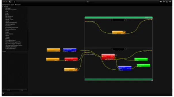
Therefore, we have introduced a visual pro-gramming tool in the platform, that allows to build a high-level computational scenario without writ-ing any line of code. Thus, for each abstraction defined in the platform, a visual wrapping (node) is introduced, which can be handled in the composer space, and connected to other nodes to construct the desired computational scenario (see Fig. 2). For a given node, several plugins may exist, that correspond to various implementations, and can be selected using the composer. This approach is hierarchical, in the sense that a node can contain itself a composition based on other nodes. More-over, particular nodes represent control structures, such for loops, if then conditions, etc.
Figure 2: Illustration of the visual programming system.
This visual programming approach really facil-itates the introduction of a new user. Moreover, it represents a valuable tool to prototype a new computational scenario. It should be underlined that the frontier between visual programming (us-ing the composer) and inline programm(us-ing (imple-mentation in plugins) completely depends on the choice of the user: it is possible to program en-tirely the simulation process using the composer and, on the contrary, it is also possible to embed a whole simulation process into a unique plugin. Of course, an intermediate choice is usually more useful. Performance studies have been conducted to quantify a possible loss of performance due to
the use of such a visual programming tool. How-ever, it has been found that this loss of perfor-mance is negligible.
1.3 Graphical interface and scientific visualization
The graphical interface is composed of four main spaces: the composer space that allows to visually build a computational scenario, the visu-alization space used for scientific visuvisu-alization of computational results and two other spaces dedi-cated to data exchange and parallel computing.
The composer space permits the user to select a node among a set of existing nodes, drop it in a working space, select the desired implementation in a corresponding plugin (see Fig. 2), and connect it with other nodes to construct a given computa-tional scenario.
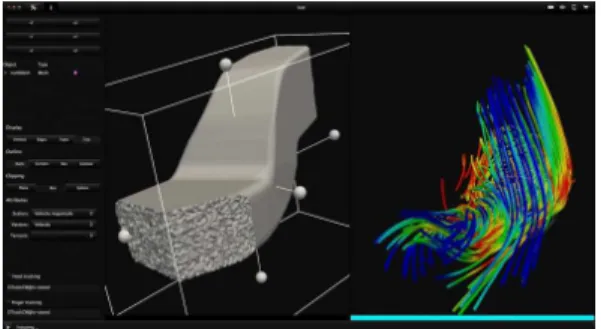
The visualization tool is based on the well-known VTK library (http:://www.vtk.org) and contains all usual features to visualize scalar or vectorial fields, glyphes or streamlines, grid nodes, faces, edges, etc (see Fig. 3). The main important feature is that an object can be visualized as soon as it is computed. Actually, the view itself is con-sidered as a node in the composition which is fed by grids, fields, etc. Therefore, each time a field is updated, the modifications can be seen in the visualization space. This feature, associated with the possibility to change a parameter or a plugin at runtime, makes the interactive computation and visualization possible.
Figure 3: Illustration of the visualization space.
1.4 Stereoscopic visualization
The researches related to methods used to visu-alize 3D fields have known a growing interest for the last years. Indeed, simulated flows are more and more complex and the use of sophisticated turbulence models, such as LES (Large Eddy Sim-ulation), DES (Detached Eddy Simulation) or VMS (Variational Multi-Scale) models requires visual-ization tools that help to capture the main
char-acteristics of the flow. Among all the possible ap-proaches, the use of virtual reality facilities is ex-plored. INRIA Sophia Antipolis M ´editerran ´ee cen-ter has an immersive space facility, which regroups two display devices, a CadWall for its ease of use and an iCube for its immersion quality. This fa-cility is dedicated to research in virtual reality, but can also be used by non-specialists to explore the possibilities of these new visualization devices.
The CadWall employed for the present ex-periments can be seen as a single screen of 3528x1200 pixels. Two images are simultaneously projected onto the wall and allows to create a 3D perception of the objects by using specific glasses. A dedicated software layer has been introduced in the platform in order to make the generation of such a stereoscopic view possible. Then, the plat-form can be used with the CadWall, or with any classical screen, without any modification.
Figure 4: Virtual reality facility at INRIA Sophia An-tipolis M ´editerran ´ee center.
2. APPLICATION TO COMPRESSIBLE FLOW SIMULATION
We explain in this section how the proposed software architecture is used for compressible flow simulation. We present first the numerical methods employed and then how they are imple-mented in the platform and plugins. Note that the platform is not devoted to CFD, fluid mechan-ics is only an application among others. At the present time, the platform is used by two INRIA Project-Teams for computations in aerodynamics (finite-volume method), electromagnetics (discon-tinuous Galerkin method), pedestrian traffic mod-eling (finite-volume method) and thermal conduc-tion (finite-element method). Moreover, the com-putational scenario is not restricted to simulation, but other computations can be carried out, on the basis of the same software components.
2.1 Modelling and numerics
Modeling The equation solved for compressible flows simulation are the Navier-Stokes equations. In conservative form, they can be written as:
∂tWc+ ∇ · F (Wc) = ∇ · N (Wc) + S(Wc) (1)
with the conservative variables Wc =
(ρ, ρu, ρv, ρw, ρE)T, the inviscid flux F(Wc) =
(F (Wc), G(Wc), H(Wc))T, the viscous flux
N (Wc) = (R(Wc), S(Wc), T (Wc))T and the
source term S(Wc).
The components of the inviscid flux in the global frame R0(bx, by, bz) are: F(Wc) = ρu ρu2+ p ρuv ρuw u(ρE + p) , G(Wc) = ρv ρvu ρv2+ p ρvw v(ρE + p) H(Wc) = ρw ρwu ρwv ρw2+ p w(ρE + p) The components of the viscous flux are:
R(Wc) = 0 τxx τxy τxz uτxx+ vτxy+ wτxz+ qx S(Wc) = 0 τyx τyy τyz uτyx+ vτyy+ wτyz+ qy T(Wc) = 0 τzx τzy τzz uτzx+ vτzy+ wτzz+ qz To close the equations, the pressure is modeled by the perfect gas state lawE = p
(γ−1)ρ+ 1
2V · V, the
heat flux q is modeled by using a Fick or Fourier law q(ǫ, κ) = −γµPr∇ǫ, the adiabatic index is set to γ = 1.4, the Prandtl number is set to Pr = 0.72 and the viscosity µ is either assumed to be constant or modeled with the Sutherland law. By neglect-ing the viscous fluxes and the source term in the equation 1, the Euler equations are recovered.
Spatial discretization A Mixed finite-Element/finite-Volume (MEV) discretization is used, which consists in discretizing the domain with a mixed finite-element/finite-volume approach of vertex centered type. The inviscid fluxes are discretized with a finite-volume approach while the viscous fluxes are discretized with a finite-element approach [2, 3].
A polygonal bounded domain Ω ⊂ Rn is
considered with a bound Γ, sub-divided into a tetrahedrization or triangulation Th with elements
Ti. Around each vertexsi a finite-volume control
cell Ci of a measure m(Ci) is constructed. The
set of vertices which are joined to the vertexsi is
denoted by N(si). The subset of all the highest
topological dimension polygons sharing the vertex siis denoted by T(si).
The inviscid fluxes are computed on the dual control cellsCi while the viscous fluxes are
com-puted on the elements Ti. A weak formulation of
the Navier-Stokes equations can be expressed us-ing a Galerkin approach.
By integrating the equation 1 over a control cellSi
(dual control cell or element) against a regular test functionϕi, the weak formulation is written as:
Z Si (∂tWc+ ∇ · F (Wc))ϕidΩ = Z Si (∇ · N (Wc))ϕidΩ + Z Si (S(Wc))ϕidΩ (2)
The finite-volume method can be interpreted as a Galerking method with the control cellSi = Ci
and with the test function equals 1 inside the dual control cell and 0 outside. This test function, re-lated to the control cellCi is defined as:
ϕCi (x) =
(
1, if x is in Ci
0, else
The variables Wcare considered to be constant
on each control cellsCi. These constants are
de-noted by Wc
i on the cellCi (see Fig. 5 and Fig.
6).
By using the Green-Ostrogradski theorem, the left term of 2 becomes:
Z Ci (∂tWc+ ∇ · F (Wc))ϕCi dΩ = m(Ci)∂tWic+ Z ∂Ci (F (Wc ) · bη))dσ (3)
with bηthe outward unit normal on∂Ci, the
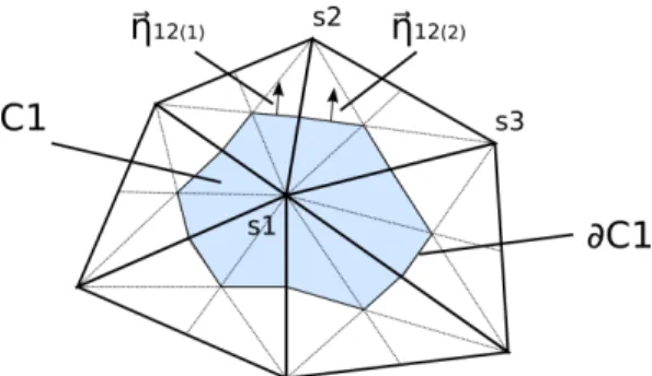
Figure 5: Illustration of a control cell in 2D.
Figure 6: Illustration of a control cell in 3D.
Furthermore, as the domain is discretised, Z ∂Ci (F (Wc ) · bη))dσ = X sj∈N (si) Z ∂Ci∩∂Cj (F (Wc ) · bη))dσ ≈ X sj∈N (si) F (Wc) |ij· Z ∂Ci∩∂Cj b ηdσ = X sj∈N (si) F (Wc) |ij· ηij (4) The F(Wc)
|ij part is modeled by using an
ap-proximate Riemann solver for which the associ-ated numerical flux is Φij = Φ(Wic, W
c j, ηij).
In the current work, the Rusanov, Steger-Warming [8, 1, 9] numerical fluxes are used.
To reach a high-order approximation in space, a MUSCL reconstruction technique is used. The reconstructed primitive state from Wipat the com-mon interface of the cells Ci and Cj is denoted
by Wijp: Wijp = Wip + 1
2αij(∇W p
i ) · IJ . The
slope (∇Wip) · IJ is approximated by ∆Wip =
2/3∆|NWip + 1/3∆|CWijp. The nodal slope
∆|NW p
i is computed from the nodal P1-Galerkin
gradients that is the average gradient of the gra-dients computed on the elementsT ∈ T (si). The
slope∆|CWijp corresponds to the centered slope
Wjp− Wip. We denoteαij(∆|NWip, ∆|CW p ij) the
limiting coefficient. Note that the reconstruction is performed using primitive variables and not con-servative variables.
Finally, the high-order numerical flux becomes: ΦijHigh order= Φ(Wijc, W
c ji, ηij).
The finite-element method can be retrieved by using the control cellSi = Ti and by using basis
functions on the element as test functions. The polygon Ti is defined as a Lagrange P1 finite
el-ement with a canonical basis denoted by ϕTi for each vertexsi. The local basis functionϕTi is equal
to 1 at vertexsi and zero at the other vertices of
the element.
A P1approximation of any functionf on a polygon
Ti can be done by projecting it on the canonical
basisϕT of the polygon:
f (X) ≈ fTi h (X) =< f, ϕ T >= NXs∈Ti i=1 f (i)ϕT i (X)
A linear approximation on each polygon Ti is
se-lected by using linear polynomial functions defined by the set P1.
This approximation is used for the density, the velocity and the temperature (or equivalently the internal energy).
By integrating by part, and by using the Green-Ostrogradski theorem, the diffusive term of 2 be-comes: Z Ti (∇ · N (Wc))ϕTidΩ = − Z Ti N (Wc ) · ∇ϕTidΩ + Z ∂Ti (N (Wc) · n)ϕT idσ (5) The velocity gradient being assumed to be con-stant by element, and ∇ϕT
i being a constant: Z Ti N (Wc) · ∇ϕT idΩ = N (Ti) · ∇ϕTi Z Ti dΩ = N (Ti) · ∇ϕTim(Ti) (6) By denoting ηTi = −ϕ T
im(Ti), the viscous
nu-merical flux is defined as:
Thus the equation 5 becomes: Z Ti (∇ · N (Wc))ϕT idΩ = ΥTi+ Z ∂Ti (N (Wc) · n)ϕTidσ (8) The term R∂T i(N (W c) · n)ϕT idσ concerns the
boundary conditions for the viscous terms.
Time integration An implicit second-order time discretization is obtained by using a dual time step approach and a backward time integration. The dual time step approach is similar to the one pro-posed in [4]. We introduce the computed residual Rifor the control celli. By denoting δ2
1Λ = Λ2−Λ1
the variation of the variable Λ from the state 1 to the state 2, we obtain as second-order implicit time integration scheme: m(Ci) 3Wc i n+1− 4Wc i n+ Wc i n−1 2δn+1n t + Ri(Wcn+1) = 0 (9) To solve this problem we introduce a subiteration state of indexk, such as:
Wicn+1= lim
k→∞W c i
(k+1)
The linearization of 9 around the state of indexk, with a local time stepδkk+1tiyields:
m(Ci) δkk+1ti +3m(Ci) 2δn+1n t ! In+ J∗(Wc(k)) ! δk+1k Wic = −Ri(Wc(k)) + m(Ci) δn n−1Wic− 3δ k nWic 2δn+1n t (10) with J∗(Wc(k)) an approximate Jacobian of the
numerical fluxes. It is composed of an inviscid and a viscous part. The inviscid Jacobian is based on the first-order Rusanov flux. The use of the Ru-sanov flux, or spectral radius Jacobian approxima-tion, is usually used in matrix-free approaches [5]. The viscous Jacobian is based on the exact Jaco-bian of the viscous fluxes and is computed as in [2].
The resulting Jacobian matrix is inversed with either a Jacobi or a symmetric Gauss-Seidel iter-ative algorithm. The use of a delta form for the implicit formulation allows to use an approximated Jacobian without loosing the second order accu-racy in space reached with MUSCL extrapolation.
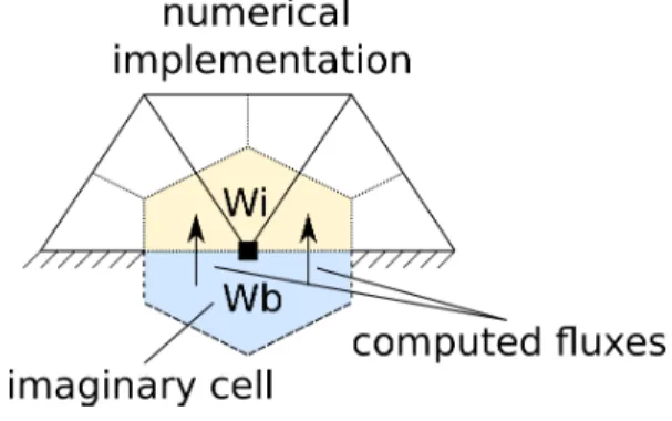
Boundary conditions The boundary conditions are implemented in a weak form through numerical fluxes. The representation of this implementation is given on the Fig. 7.
Figure 7: Illustration of the implementation of weak boundary conditions.
The flux computed between the fictive state Wc b
and the boundary (or interior) state Wc
i can be
computed with any numerical flux (independently from the interior fluxes). Depending on the bound-ary condition used, the fictive state Wc
b can be a
function of the interior and the exterior state Wc o: Wc b = W c b(W c i, W c
o). In this study, the
com-putation of the fictive state is carried out using the Riemann invariants for free-stream conditions, imposed pressure with extrapolation of charac-teristics for subsonic outlets (characteristic based methods), and symmetry conditions for slipping walls.
The non-slip condition is strongly imposed by setting a zero velocity on the boundary. The Jaco-bian matrix is thus modified such that the bound-ary velocity does not evolve.
The viscous boundary fluxes are neglected for free-stream boundary conditions and computed for other cases.
2.2 Possible implementation levels
The numerical methods presented above can be implemented in the platform and plugins with dif-ferent integration levels. On the one side, we can construct a simple composition based on sophis-ticated plugins, that basically represent the mesh generator, the solver and the view. On the other side, we can also construct a sophisticated com-position based on simple plugins, that represent all single operations performed during the compu-tational scenario. Using the former approach the visual programming tool is not much employed, whereas using the latter approach it is intensively used.
Actually, we choose an intermediate level, that allows to obtain a modular implementation where needed by our research topic. The whole mesh generator is embedded in a single plugin, whereas the solver is partitioned into elementary plugins. Therefore, the loops over finite-volume control cells or finite-elements are defined by the com-poser, while the local computations of fluxes, Ja-cobians, time-steps, etc. are embedded into ele-mentary plugins. We obtain finally a quite sophisti-cated composition, presented in Fig. 8, which con-tains sub-compositions, such as the one illustrated in Fig. 9 used to compute and store the inviscid flux and the local time step for a given pair of con-trol cells.
Figure 8: Composition used for flow simulation.
Figure 9: Sub-composition used for flux and local time step computation and storage.
2.3 Interaction parameters
As explained above, the user can interact with the computation by modifying at runtime a plugin or its parameters. In the case of compressible flow simulations, we have so far used three different ways to modify interactively the computations:
• Modification of a plugin to change the algo-rithm used. For instance, we change the nu-merical flux or the limiting coefficient function;
• Modification of a parameter of a plugin to change boundary conditions. For instance, we change free-stream velocity, or pressure; • Modification of a parameter of a plugin to
change a numerical method. For instance, we increase or decrease the CFL number used to compute the time step.
All these modifications are performed using a graphical interface in the composer space. Illus-trations are provided in the next sections.
3. SOME ILLUSTRATIONS
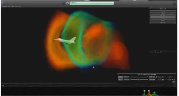
3.1 Sonic boom crossing for F16 aircraft
As first illustration, we consider the three-dimensional inviscid compressible flow around a F-16 aircraft. The computational scenario chosen here, with which the user interacts, is not the res-olution of the state equation, but the construction of a reduced order model from a flow database. A set of 16 computations have been performed and stored, with a grid of about 230,000 nodes, for dif-ferent values of incidence and free-stream velocity. Then, the visual programming tool is used to con-struct a scenario that reads these solutions, inter-polates linearly the solutions to compute flow vari-ables for a given angle of attack and free-stream velocity, and visualize the data of interest. Using some widgets, the user can modify the angle of attack and the free-stream velocity, while the visu-alization is updated interactively.
Figure 10: Pressure isolines for F16 aircraft.
To obtain a suitable perception of 3D fields, a volumic rendering feature is implemented in the platform, which lets the user control the color and transparency associated to each field value. The scalar field of interest is evaluated on a cartesian grid from the flow solution and updated as the user modifies the interaction parameters. This task is carried out using GPUs, in order to obtain a satis-factory rendering.
Figure 11: Pressure field in subsonic regime.
Figure 12: Pressure field in supersonic regime.
Figure 13: Modification of the volume rendering lookup table to isolate shock waves.
The pressure isolines on the aircraft surface in subsonic regime are illustrated in Fig. 10. The use of the volume rendering technique to obtain a 3D perception of the pressure field is shown on Fig. 11. As the user increases the free-stream velocity, the flow becomes supersonic and three shock waves appear, on the nose, the wing and the tail of the aircraft (see Fig. 12). It is possi-ble to modify the lookup tapossi-ble used for the volumic rendering to isolate the different shock waves, as illustrated in Fig. 13.
3.2 Supersonic ramp
In the previous example, the user interacts with a reduced order model of the flow fields. Now, we would like to illustrate the possible interaction with the PDE solver itself. We consider the invis-cid supersonic flow over a15◦ramp, for inlet con-ditions corresponding to a Mach number of value Min = 2. The grid counts about 2,500 nodes. An
unsteady simulation is performed in order to ob-serve the flow development. During a first phase,
one can observe the development of a shock wave and a rarefaction wave (see Fig. 14). Then, the shock is reflecting on the opposite wall and the flow converges to the solution depicted in Fig. 15. At this time, the user modifies the inlet boundary conditions using the widgets located at the left of the visualization space: the Mach number is pro-gressively increased to Min = 3. The inlet flow
change is progressing in the tunnel and modifies the shock wave characteristics, as illustrated in Fig. 16.
Figure 14: Pressure field: shock wave and rarefac-tion wave in development.
Figure 15: Pressure field: shock wave reflecting.
Figure 16: Pressure field: interaction between inlet condition change and shock wave.
This experiment illustrates how the user can in-teract with a computation at runtime and visualize simultaneously the flow modifications. The change
of boundary condition value has been demon-strated here, but we can consider other types of interaction: the user can for instance modify the boundary condition type or location, or even mod-ify numerical parameters, such as the numerical flux evaluation or the time step.
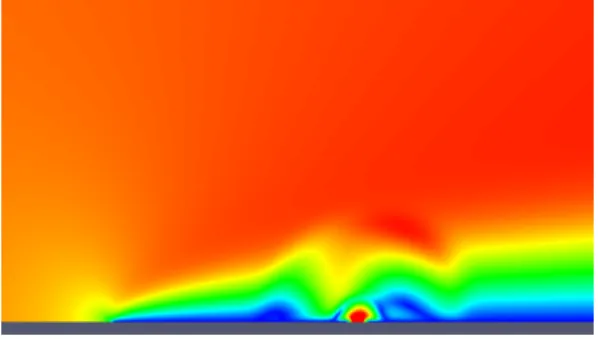
3.2 Oscillatory jet actuation
Finally, we present the interactive simulation of a viscous compressible flow. We consider the laminar flow over a flat plate, well known as Bla-sius test-case, and we introduce an oscillatory suction/blowing jet. The free-stream Mach num-ber is Min = 0.3 and the Reynolds number is
Re = 100 (based on the distance δ between the leading edge and the jet location) . The oscillatory jet width isδ/10 and frequency f = 10. The grid counts about 8,000 nodes. A second-order time integration is employed, with a physical time step 5 10−4.
Figure 17: Velocity modulus without actuation (t0).
Figure 18: Velocity modulus (t0+ 0.015).
During a first phase of the simulation, no actu-ation is done. A boundary layer is developing, as illustrated in Fig. 17. Then, at a timet0, the user
decides to activate the actuation. This is done by setting a non-zero actuation amplitude for the plu-gin that computes the jet boundary conditions (see Fig. 18). For the next time steps, the oscillatory
Figure 19: Velocity modulus (t0+ 0.040).
Figure 20: Velocity modulus (t0+ 0.060).
Figure 21: Velocity modulus (t0+ 0.085).
Figure 22: Velocity modulus (t0+ 0.120).
blowing / suction boundary conditions modify sig-nificantly the boundary layer, as can be seen in
Fig. 19 to Fig. 22. Although this is not presented here, the user can also modify the actuation fre-quency interactively.
DISCUSSION AND CONCLUSION
A modern software architecture, based on a platform / plugins system and a visual program-ming tool, has been used to implement numerical methods for compressible flow simulations. The platform features allow the user to modify interac-tively the computations by changing some param-eters or even some plugins at runtime, while ob-serving the impact on the solution.
Some tests have been carried out, that deal with reduced-order model construction for the 3D invis-cid flow around an aircraft, interaction with inlet boundary conditions for the supersonic flow over a ramp, and finally modification of an oscillatory jet for a boundary layer flow.
These tests have shown that interactive compu-tation and visualization in CFD is possible and is beneficial from a scientific point of view:
• a better understanding of physical phenom-ena or numerical behaviors is obtained; • the use of CFD tool is more attractive for
non-experts;
• the adjustment of physical or numerical pa-rameters is easier.
Of course this approach is limited by the com-putational facility used. Presently, for a sequential approach, the interactive computation is satisfac-tory until some dozen of thousand nodes. There-fore, we are presently implementing the use of par-allel approaches in the platform, to be able to apply interactive computation to large-scale problems. Our objective is to study interactively turbulent flows, by using simultaneously high-performance computing and virtual reality facilities.
References
[1] BATTEN, P., CLARKE, N., LAMBERT, C.,AND
CAUSON, D. On the choice of wavespeeds
for the hllc riemann solver. SIAM Journal on Scientific Computing 18 (1997), 1553. [2] FEZOUI, FATIMA, L., LANTERI, S., LAR
-ROUTUROU, B.,ANDOLIVIER, C. Resolution
numerique des equations de Navier-Stokes pour un fluide compressible en maillage tri-angulaire. Rapport de recherche RR-1033, INRIA, 1989.
[3] FRANCESCATTO, J. M ´ethodes multigrilles par agglom ´eration dirrectionnelle pour le cal-cul d’ ´ecoulements turbulents. PhD thesis, Universit/’e de Nice-Sophia Antipolis, Nice, France, 1998.
[4] JAMESON, A. Time dependent calculations using multigrid, with applications to unsteady flows past airfoils and wings. AIAA paper 91 (1991), 1596.
[5] KLOCZKO, T. D ´eveloppement d’une m ´ethode
implicite sans matrice pour la simulation 2D-3D des ´ecoulements compressibles et faiblement compressibles en maillages non-structur ´es. PhD thesis, Arts et M ´etiers Paris-Tech, 2006.
[6] KREYLOS, O., TESDALL, A. M., HAMANN, B., HUNTER, J. K.,ANDJOY, K. I. Interactive vi-sualization and steering of cfd simulations. In 8th Eurographics Workshop on Virtual Envi-ronments (2002).
[7] SCHIRSKI, M., GERNDT, A., VAN REIMERS
-DAHL, T., KUHLEN, T., ADOMEIT, P., LANG, O., PISCHINGER, S.,ANDBISCHOF, C. Vista
flowlib a framework for interactive visualiza-tion and exploravisualiza-tion of unsteady flows in vir-tual environments. In 7th International Im-mersive Projection Technologies Workshop, Zurich, Switzerland, 22–23 May, 2003 (2003). [8] STEGER, J. L., AND WARMING, R. Flux vector splitting of the inviscid gasdynamic equations with application to finite-difference methods. Journal of Computational Physics 40, 2 (1981), 263 – 293.
[9] TORO, E., SPRUCE, M., AND SPEARES, W. Restoration of the contact surface in the hll-riemann solver. Shock waves 4, 1 (1994), 25– 34.
[10] WENISCH, P., BORRMANN, A., RANK, E.,
VAN TREECK, C., AND WENISCH, O.
Col-laborative and interactive cfd simulation using high performance computers. In 18th Sym-posium AG Simulation (ASIM) and EuroSim. Erlangen, Germany (2005).