Laboratory investigation of the fracture behaviour polycrystalline ice in indentation tests: part 1 phase 1 testing

(1)

Publisher’s version / Version de l'éditeur:

Vous avez des questions? Nous pouvons vous aider. Pour communiquer directement avec un auteur, consultez la Questions? Contact the NRC Publications Archive team at

PublicationsArchive-ArchivesPublications@nrc-cnrc.gc.ca. If you wish to email the authors directly, please see the first page of the publication for their contact information.

https://publications-cnrc.canada.ca/fra/droits

L’accès à ce site Web et l’utilisation de son contenu sont assujettis aux conditions présentées dans le site LISEZ CES CONDITIONS ATTENTIVEMENT AVANT D’UTILISER CE SITE WEB.

Technical Report (National Research Council of Canada. Institute for Ocean Technology); no. TR-2006-25, 2007

READ THESE TERMS AND CONDITIONS CAREFULLY BEFORE USING THIS WEBSITE.

https://nrc-publications.canada.ca/eng/copyright

NRC Publications Archive Record / Notice des Archives des publications du CNRC :

https://nrc-publications.canada.ca/eng/view/object/?id=1f75b3f9-aa4c-43a8-9742-36b221559f5d https://publications-cnrc.canada.ca/fra/voir/objet/?id=1f75b3f9-aa4c-43a8-9742-36b221559f5d

NRC Publications Archive

Archives des publications du CNRC

For the publisher’s version, please access the DOI link below./ Pour consulter la version de l’éditeur, utilisez le lien DOI ci-dessous.

https://doi.org/10.4224/8896217

Access and use of this website and the material on it are subject to the Terms and Conditions set forth at

Laboratory investigation of the fracture behaviour polycrystalline ice in indentation tests: part 1 phase 1 testing

(2)

DOCUMENTATION PAGE REPORT NUMBER

TR-2006-25

NRC REPORT NUMBER DATE

January 2007

REPORT SECURITY CLASSIFICATION

Unclassified

DISTRIBUTION

Unlimited

TITLE

LABORATORY INVESTIGATION OF THE FRACTURE BEHAVIOR OF POLYCRYSTALLINE ICE WITH EMBEDDED MONOCRYSTALS – PHASE I

AUTHOR(S)

Jennifer Wells, Ian Jordaan, Ahmed Derradji-Aouat, Austin Budgen

CORPORATE AUTHOR(S)/PERFORMING AGENCY(S)

Institute for Ocean Technology, National Research Council, St. John’s, NL

PUBLICATION

SPONSORING AGENCY(S)

Institute for Ocean Technology, Marine Institute

IOT PROJECT NUMBER

2118

NRC FILE NUMBER KEY WORDS

grain boundaries, indentation tests, pressure

PAGES x, 133, App. 1-8 FIGS. 146 TABLES 4 SUMMARY

A series of indentation tests were performed as a joint collaboration between Memorial University of Newfoundland and The Institute for Ocean Technology (NRC-IOT). The tests were performed on ice specimens with dimensions of 20 x 20 x 10 cm, which were made of polycrystalline ice with a grain size of ~ 4 mm. In order to explore the role of grain boundaries, the test specimens included 2 cm cubed monocrystals placed at specific locations within the specimen. It is hypothesized that the large grain boundaries provided by the monocrystal will help to precipitate a fracture in the vicinity of the crystal. This should affect both the maximum load attainable during the test as well as the maximum duration of the tests as compared to a specimen that does not contain an embedded crystal. The tests were performed using an MTS located at the NRC-IOT. The total force was recorded during the tests using a 25 kN load cell with a sampling frequency of 20 kHz. A high-speed video camera was used in these tests to identify the location where fracture begins. A vertical sheet of laser light was used to aid in this process. The high-speed video was also used to help find a correlation between fluctuations in the load traces and visual events such as crushing, spalling and fracture. Additionally, the tests included the use of a tactile pressure sensor in the indentation area. The sensor was included in order to explore the pressure distribution in the area of the indenter. This area was found to consist of isolated areas of very high pressure compared to the average pressure found during the test.

ADDRESS National Research Council

Institute for Ocean Technology Arctic Avenue, P. O. Box 12093 St. John's, NL A1B 3T5

(3)

National Research Council Conseil national de recherches Canada Canada Institute for Ocean Institut des technologies Technology océaniques

LABORATORY INVESTIGATION OF THE FRACTURE BEHAVIOR OF

POLYCRYSTALLINE ICE WITH EMBEDDED MONOCRYSTALS –

PHASE I

TR-2006-25

Jennifer Wells, Ian Jordaan, Ahmed Derradji-Aouat, Austin Bugden

(4)

TABLE OF CONTENTS

List of Figures ... iv

List of Tables... x

1.0 Introduction... 1

2.0 Specimen preparation... 1

3.0 Test parameters / Test Matrix ... 3

4.0 Experimental Setup and Instrumentation... 5

5.0 Post-Test Thin Sections ... 8

6.0 Experimental Results ... 10

7.0 Recommendations for Analysis ... 13

8.0 References... 15

Appendix 1: Test parameters and sample preparation... 17

Appendix 2: Indenter Displacement ... 23

Appendix 3: High-Speed Video Stills and Post-Test Photographs... 31

Appendix 4: Thin-Sections ... 59

Appendix 4: Load Traces... 77

Appendix 5: Mean Nominal Stress ... 91

Appendix 6: Pressure Sensor Data... 99

Appendix 8: Calibrations ... 125

Pressure Sensor ... 125

Conditioning ... 125

Equilibrating ... 125

Calibration... 125

Calibration for piezoelectric load cell... 127

(5)

LIST OF FIGURES

Figure 1: Seed ice with an average grain diameter of ~ 4mm, used to produce the

polycrystalline ice used in the tests... 19

Figure 2: (a) Fiberglas mold used in the production of the ice specimens. (b) Glass bead used as a depth marker in the unfinished ice specimen. ... 19

Figure 3: Schematic representation of (a) the molded specimen of ice prior to and post machining. Each molded specimen was machined to produce two final test specimens. Note that 2 cm cubed monocrystals were placed at predetermined locations and marked using glass depth markers, which were removed by the machining process. (b) The embedded monocrystals were placed at predetermined depths within the molded specimen. They were located at a vertical depth of 10 mm within each specimen and at three horizontal locations corresponding to the predetermined indentation locations. ... 20

Figure 4: (a) MTS located at the NRC-IOT (b) Tekscan I-Scan pressure sensor system 21 Figure 5: Photograph of the setup used in the experiments. ... 21

Figure 6: (a) microtome used in the production of the post-test thin sections. (b) Light table used in the photography of the thin sections... 22

Figure 7: Indenter displacement as a function of time for I06_V2P0_I_025 ... 23

Figure 8: Indenter displacement as a function of time for I06_V2P0_C_026 ... 23

Figure 16: Indenter displacement as a function of time for I06_V2P0_E_035 ... 27

Figure 20: Photograph taken prior to test I06_V2P0_I_025 that shows the green laser pointer being used to generate a vertical sheet of laser light, in the same plane as the embedded crystal. ... 31

Figure 21: Photograph taken prior to test I06_V2P0_I_025 that shows how the vertical sheet of laser light can be used to illustrate the position of the embedded monocrystal. The crystal can be seen as a void in the light, directly underneath the indenter. ... 32

Figure 22: Sequence of frames taken from the high-speed video of I06_V2P0_I_025.... 32

Figure 23: Sequence of frames taken from the high-speed video of I06_V2P0_C_026. . 33

Figure 27: Sequence of frames taken from the high-speed video of I06_V10P0_C_030. 37 Figure 28: Sequence of frames taken from the high-speed video of I06_V10P0_I_031.. 38

(6)

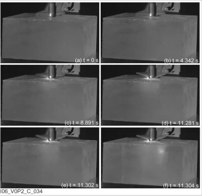
Figure 30: Sequence of frames taken from the high-speed video of I06_V0P2_C_034. . 40

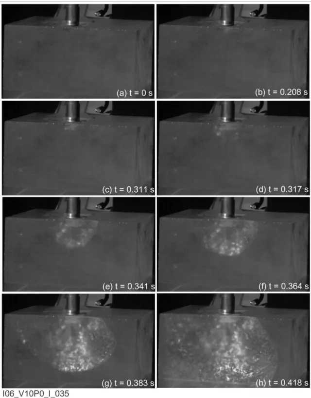
Figure 31: Sequence of frames taken from the high-speed video of I06_V10P0_I_035.. 41

Figure 33: Sequence of frames taken from the high-speed video of I06_V10P0_E_037. Arrow points to void left by embedded crystal... 43

Figure 34: Sequence of frames taken from the high-speed video of I06_V2P0_E_038. . 44

Figure 35: Experimental stills taken immediately after testing of I06_V2P0_I_025. ... 45

Figure 36: Experimental stills taken immediately after testing of I06_V2P0_C_026... 46

Figure 40: Experimental stills taken immediately after testing of I06_V10P0_C_030.... 50

Figure 41: Experimental stills taken immediately after testing of I06_V10P0_I_031. .... 51

Figure 42: Experimental stills taken immediately after testing of I06_V10P0_C_032.... 52

Figure 45: Experimental stills taken immediately after testing of I06_V2P0_E_035. ... 55

Figure 49: Schematic diagram showing the fracture patterns for all intermediate tests... 59

Figure 50: Schematic diagram showing the fracture patterns for all center tests. ... 59

Figure 51: Schematic diagram showing the fracture patterns for all edge tests. ... 60

Figure 52: (a) Thin-sections from I06_V2P0_I_025 shown under polarized lighting. (b) A schematic representation of the tested specimen. The box represents the locations from which each section was removed. ... 61

Figure 52: (c) Thin-sections from I06_V2P0_I_025 shown using reflected lighting... 62

Figure 53: (a) Thin-sections from I06_V2P0_C_026 shown under polarized and reflected lighting. (b) A schematic representation of the specimen tested. The box represents the locations from which each section was removed... 63

Figure 54: (a) Thin-sections from I06_V0P2_I_027 shown under polarized and reflected lighting. (b) A schematic representation of the specimen tested. The box represents the locations from which each section was removed... 64

Figure 58: (a) Thin-sections from I06_V10P0_I_031 shown under polarized. (b) A schematic representation of the specimen tested. The box represents the locations from which each section was removed. ... 68

(7)

Figure 59: (a) Thin-sections from I06_V10P0_C_032 shown under polarized and reflected lighting. (b) A schematic representation of the specimen tested. The box

represents the locations from which each section was removed... 70

Figure 62: (a) Thin-sections from I06_V2P0_E_035 shown under polarized and reflected lighting. (b) A schematic representation of the specimen tested. The box represents the locations from which each section was removed... 73

Figure 66: Total force as a function of time for test I06_V2P0_I_025 ... 77

Figure 67: Total force as a function of time for test I06_V2P0_C_026 ... 78

Figure 68: Total force as a function of time for test I06_V0P2_I_027. ... 78

Figure 71: Total force as a function of time for test I06_V10P0_C_030. ... 79

Figure 73: Total force as a function of time for test I06_V10P0_C_032 (figure shows total force as recorded by the pressure sensor only since the MTS did not record data for this test). ... 80

Figure 76: Total force as a function of time for test I06_V2P0_E_035. ... 82

Figure 80: Total force recorded by the piezoelectric load cell as a function of time for test I06_V2P0_C_026. ... 84

Figure 81: Total force recorded by the piezoelectric load cell as a function of time for test I06_V0P2_I_027... 84

(8)

Figure 85: Total force recorded by the piezoelectric load cell as a function of time for test

I06_V10P0_C_032. ... 86

Figure 87: Total force recorded by the piezoelectric load cell as a function of time for test I06_V2P0_E_035... 87

Figure 91: Diagram showing the calculation of the nominal / projected area of the spherical indenter. The nominal area represents the area of a circle that has a radius that changes according to the depth of penetration of the indenter. ... 91

Figure 92: Mean Nominal Stress as a function of time for test I06_V2P0_I_025 ... 92

Figure 93: Mean Nominal Stress as a function of time for test I06_V2P0_C_026 ... 92

Figure 101: Mean Nominal Stress as a function of time for test I06_V2P0_E_035 ... 96

Figure 105: Maximum pressure and average pressure as a function of time for test I06_V2P0_I_025... 99

Figure 106: Maximum pressure and average pressure as a function of time for test I06_V2P0_C_026. ... 100

Figure 108: Maximum pressure and average pressure as a function of time for test ... 102

I06_V0P2_I_028... 102

(9)

Figure 114: Maximum pressure and average pressure as a function of time for test

I06_V0P2_C_034. ... 108 Figure 115: Maximum pressure and average pressure as a function of time for test

I06_V2P0_E_035... 109 Figure 116: Maximum pressure and average pressure as a function of time for test

I06_V2P0_E_038... 112 Figure 119: Screen captures from the software which accompanies the pressure sensor.

The screen shots show four different times during the evolution of the test. The white window on the left of each figure gives the pressure distribution for that particular time as a color map. The color scale within this window shows the value of the pressure at each spatial location. The gray widow on the right of each

screenshot shows the time synchronized total force. ... 113 Figure 120: maximum pressure as a function of speed for all test locations... 114 Figure 121: average pressure as a function of speed for all test locations... 114 Figure 122: maximum pressure as a function of location for all indentation velocities. 115 Figure 124: maximum total force as a function of position for all the tests using a speed

of 0.2 mm/s. ... 117 Figure 125: maximum total force as a function of position for all the tests using a speed

of 2.0 mm/s. ... 117 Figure 126: maximum total force as a function of position for all the tests using a speed

of 10.0 mm/s. ... 118 Figure 127: maximum test duration as a function of position for all the tests using a speed of 0.2 mm/s. ... 119 Figure 128: maximum test duration as a function of position for all the tests using a speed of 2.0 mm/s. ... 119 Figure 129: maximum test duration as a function of position for all the tests using a speed of 10.0 mm/s. ... 120 Figure 130: maximum total force as a function of indentation speed for all the tests

performed at a center location... 121 Figure 131: maximum total force as a function of indentation speed for all the tests

performed at an edge location... 121 Figure 132: maximum total force as a function of indentation speed for all the tests

performed at an intermediate location. ... 122 Figure 133: maximum total force as a function of indentation speed for tests performed at

all locations. ... 122 Figure 134: maximum test duration as a function of indentation speed for all the tests

performed at a center location... 123 Figure 135: maximum test duration as a function of indentation speed for all the tests

performed at an edge location... 123 Figure 136: maximum test duration as a function of indentation speed for all the tests

(10)

Figure 137: maximum test duration as a function of indentation speed for tests performed

at all locations. ... 124

Figure 138: Sample calibration plot for the piezoelectric load cell. The upper plot gives the load trace in volts recorded by the piezoelectric load cell. The lower plot gives the load trace in Newtons recorded by the strain-gauge load cell. ... 128

Figure 139: MTS calibration certificate... 129

Figure 140: Secondary MTS calibration certificate... 130

Figure 141: Certificate of calibration showing traceability to national standard... 131

Figure 142: Secondary calibration certificate for load cell... 132

Figure 143: Piezoelectric load cell calibration... 133

Figure 144: Strain-gauge load cell calibration... 134

Figure 145: LVDT calibration. ... 135

(11)

LIST OF TABLES

Table 1: Summary of parameters used for each test. ... 17 Table 2: Labels and information for each test. ... 17 Table 3: Summary of temperatures recorded during testing. The air temperatures were

recorded close to, but not in contact with the MTS. The piston temperature was located on the MTS, but does not give the temperature of the horizontal platform on which the samples were resting. ... 18 Table 4: Drift values calculated by taking the amount of drift in volts / second for

(12)

1.0 INTRODUCTION

The tests described herein involved a series of indentation tests that were performed as a joint collaboration between Memorial University of Newfoundland and The Institute for Ocean Technology (NRC-IOT). The tests were performed on ice specimens with dimensions of 20 x 20 x 10 cm, which were made of polycrystalline ice with a grain size of ~ 4 mm. In order to explore the role of grain boundaries, the test specimens included 2 cm cubed monocrystals placed at specific locations with in the specimen

The tests were performed using an MTS located at the NRC-IOT. The total force was recorded during the tests using a 25 kN load cell with a sampling frequency of 20 kHz. A high-speed video camera was used in these tests to identify the location where fracture begins. A vertical sheet of laser light was used to aid in this process. The high-speed video was also used to help find a correlation between fluctuations in the load traces and visual events such as crushing, spalling and fracture.

Additionally, the tests included the use of a tactile pressure sensor in the

indentation area. The sensor was included in order to explore the pressure distribution in the area of the indenter. This area was found to consist of isolated areas of very high pressure compared to the average pressure found during the test.

2.0 SPECIMEN PREPARATION

The test specimens had dimensions of 20 x 20 x 10 cm and consisted of

polycrystalline ice specimens with a grain size of ~ 4 mm that had embedded 2 cm cubed monocrystals at specific locations within the specimen. The monocrystals were

(13)

embedded at a vertical depth of either 10 mm or 20 mm within the sample and at three horizontal locations depending on the test. The depth of 10 mm was chosen because it represents the approximate depth of maximum shearing stress during the indentation. The 20 mm depth was chosen to explore the effect of varying the depth of the crystal. The specimens were prepared according to the procedure outlined in Mackey (2006). Large blocks of bubble-free ice were purchased commercially to reduce the time necessary to produce test specimens. These blocks were crushed using a commercial ice crusher and sieved using a standard ASTM International 3.35-4.75 mm sieve to obtain seed ice (Figure 1, Appendix 1). The embedded crystals were cut from a large piece of monocrystal that had been grown using distilled, deaerated water. The ice specimens were then molded using a Fiberglas mold (Figure 2 (a), Appendix 1).

Each fill of the Fiberglas mold produced two test specimens as is shown

schematically in Figure 3 (a), Appendix 1. First, the mold was partially filled with seed ice. A monocrystal was then placed in the mold such that it would be embedded in a predetermined location in the finished specimen (Figure 3 (b)). The embedded crystal was placed so that it would have a vertical c-axis in the finished specimen. Small colored glass beads were also included in the corners of the mold at the same depth, to help locate the monocrystal in the molded specimen once it had frozen. These glass depth markers were not present in the final test specimens. An example of one of the glass beads is shown in Figure 2 (b), as it appears in the ice specimen prior to finishing. More seed ice was then added to the mold as well as another monocrystal and depth markers. Enough seed ice was then added to fill the mold. The top of the mold was sealed with a flexible rubber membrane. Next, a vacuum was applied to the mold in order to evacuate air from

(14)

the inter-seed voids. Distilled and de-aerated water, at a temperature of 0 0C, was then drawn into the mold under vacuum. The mold was insulated in such a way as to promote freezing from the bottom upwards. This caused any remaining air bubbles to be pushed to the top of the mold. The ice was then allowed to freeze for at least 72 hours at –10 0C and was then removed from the mold by leaving it upturned at ~ 20 0C until it released from the mold. Once the ice released from the mold, it was immediately returned to –10 0

C for storage.

Approximately a week prior to testing, a milling machine was used to machine two test specimens, with final dimensions of 20 x 20 x 10 cm, from each molded ice (Figure 1 (a), Appendix 1). By observing the position of the glass depth markers, it was possible to ensure that the embedded crystal was located at the correct vertical and horizontal locations within the finished specimen. Additionally, since the ice had frozen from the bottom of the mold upwards, any remaining air bubbles were easily removed from the top of the ice with machining.

3.0 TEST PARAMETERS / TEST MATRIX

A total of eighteen tests were performed using a combination of differing indenter speeds and indentation locations. These test parameters were chosen to repeat the

parameters used in Mackey (2006). The tests were performed in two phases. Phase I consisted of four preliminary tests. This phase was performed in order to validate the method of specimen preparation as well as the testing procedure. Unfortunately, during the testing, an equipment malfunction occurred and as such the data from these tests was not analyzed. Due to the malfunction, the tests from this phase will not be discussed

(15)

further in this report. Visual observations that were made during the tests however were promising. It appeared that the fracture behavior was affected by the inclusion of the monocrystal and regular speed videos of the tests seemed to show fractures beginning in the area of the crystal. Therefore, a second phase was performed, which consisted of fourteen tests. The tests that were performed as part of this phase will be discussed for the remainder of the report. The parameters used for each of these tests are given in Table 1 (Appendix 1). The tests were completed using a 20 mm rigid indenter with a radius of curvature of 25.6 mm. Its shaft was painted with a matt black finish to reduce reflective glare from the lights. The indenter used in the tests is a scaled-down version of a

spherical indenter used in field tests (Frederking et al., 1990). The choice of indenter was directly related to work done by both Mackey (2006) and Barrette et al. (2003) who performed similar small-scale indenter tests on polycrystalline ice without the inclusion of embedded monocrystals.

Three different indenter speeds were used varying from 0.2 mm/s to 10 mm/s depending on the test (Table 1). The indenter displacement rates for the slow and

medium velocities were chosen to be consistent with those used by Barrette et al. (2003). In that study the fastest rate was equivalent to the medium speed in this test series. The medium speed used in this study represents a transition between ductile and brittle material behavior of the ice. The higher rate for this series was chosen to investigate the material properties beyond that transition, and into the brittle zone. Plots of the indenter displacement as a function of time are given in Appendix 1. These plots show that each test was performed using the correct predetermined velocity.

(16)

Additionally, the distance between the indentation location and the edge of the test specimen was varied to investigate any potential edge effect. A total of three indentation locations were used having distances of 2, 5 and 10 cm away from the edge of the specimen. The horizontal placement of the embedded monocrystals corresponded to these locations, with the crystal always being directly under the indentation site.

4.0 EXPERIMENTAL SETUP AND INSTRUMENTATION

The tests were conducted using a Materials Testing System (MTS) located at the NRC-IOT. The MTS setup is shown in Figure 4 (a), Appendix 1 and the entire test setup is shown in Figure 5, Appendix 1. Recent calibrations for the MTS used in this study are given in Appendix 8. The room in which the tests were completed was held at

approximately -10 0C. The exact air temperatures at the time of each test are listed in Table 3, Appendix 1. The test setup involved placing an ice specimen on the test

platform so that the indenter would make contact at the desired distance from the edge of the specimen. The indenter was than manually lowered such that it made contact with the sample, while applying negligible load to the sample. The samples were under no

confinement during the test and were conducted to a maximum actuator displacement of approximately 7 mm. The tested specimens were photographed immediately after each indentation. These photographs are included in Appendix 2. Immediately after the specimen was photographed, each piece of the fractured specimen was labeled and

packaged separately in an airtight plastic bag. A straw was used to remove as much air as possible from each bag prior to sealing. All the pieces from each specimen were then packaged together in another larger, airtight plastic bag. The specimens were then stored

(17)

in coolers with additional padding and sacrificial ice. The coolers were stored at a temperature of –10oC until thin-sectioning could begin.

The tests were controlled and recorded using the MTS controller and recording equipment (model number 448.85). A 250 kN MTS load cell (model number 661.233-01, serial number 2133) was used with a sampling frequency of 20 kHz. The load cell was deemed appropriate based on the expected loads and noise levels. This was then filtered using a 3dB cutoff frequency of 3 kHz. Additionally, a piezoelectric load cell was included in the experimental setup. This load cell had a model number PCB 237A and was conditioned using a Kistler charge amp #5010. The calibration for the piezoelectric load cell is given in Appendix 8. During each test, the MTS was used to record both the total force from the load cells and the LVDT displacement. These traces were

synchronized using a one shot synchronizing electrical pulse that was generated at the start of each test.

The tests were videotaped using 3 video cameras. Two regular speed video cameras were used - a black and white camera that recorded at 30 frames per second (fps) and a color camera that recorded at 30 fps. Also, a high-speed black and white camera that recorded at 1600, 1000 and 125 fps depending on the length of the test in question was also used. This camera was used to help establish the location where fracture

propagation begins. It was also used to help find a correlation between fluctuations in the load traces and visual events such as crushing, spalling and fracture. The videos recorded by all three cameras are available through CISTI. Appendix 2 includes a series of frames from each of the high-speed videos of the experiments. The figures clearly show the

(18)

formation and propagation of cracks as well as crushing and spalling behavior in the area of the indenter.

An extremely bright, 532 nm, green laser pointer was used to provide additional illumination during the tests. The laser beam was directed through a glass cylinder producing a vertical sheet of laser light in the plane of the embedded crystal (see Figures 7-8, Appendix 2). Figure 2 shows that this light is reflected by the many grain

boundaries in the polycrystalline ice. The location of the monocrystal is visible however since the lack of grain boundaries in this area produce a void in the sheet of light. The intention of this sheet of light is to provide evidence for the fracture being precipitated by the large grain boundary. Any fractures that begin inside the sample in the area of the crystal should reflect this light more strongly than the surrounding grain boundaries at the moment of fracture. It was originally intended that this light would provide the sole illumination during the test. Once testing began however, illuminating the specimen with only the laser lighting proved impractical. High-speed video requires significantly more light than regular speed video and as such, in order to use only the laser light, the frame rate of the high-speed video would have to be dramatically reduced. It was decided that while additional lighting would be used during the tests, the laser sheet would still be used such that the direct lighting of the crystal would show any crack formation.

Synchronization between the data collected by the MTS load cell and the high-speed video was achieved using a MiDAS data acquisition system. A one shot synchronizing electrical pulse was generated at the beginning of each test. This pulse simultaneously triggered both the initiation of the indenter and the initiation of the high-speed video. The MiDAS system then acquired the data that was being recorded for the

(19)

load and the indenter displacement and synchronized it to the high-speed video that was being captured by the camera. As a precautionary measure, the synchronizing pulse was also used to cause an LED located next to the ice specimen to flash. This process could potentially be used to manually synchronize the load data with the high-speed video but was found to be unnecessary in this case.

Additionally, the experimental set up included a Pressure sensor. The Tekscan I-Scan system (http://www.tekscan.com/industrial/iscan_specs.html) was used to record pressure and force during the tests (Figure 4 (b), Appendix 1). The system consists of a thin, flexible, resistance based sensor that was connected to an external PC. The sensor consisted of an array of 44 x 44 ‘sensels’. These sensels represent the intersection of lines of semi-conductive ink that are drawn onto the sensors in a grid pattern. The sensor had a thickness of 0.004” where there is ink present and a thickness of 0.002” where there is no ink. Measurements were taken by recording the changes in current flow at each sensel giving the applied force distribution. Using the I-Scan system, it is possible to record the force distribution at a rate of up to 100 frames per second. The pressure distribution is then calculated using the applied force and total contact area for each time. The pressure sensitive film used in these tests had a pressure rating of 25,000 PSI.

During these tests, the pressure sensor was placed between the indenter and the surface of the ice. The calibration of the sensor is described in appendix 8.

5.0 POST-TEST THIN SECTIONS

Due to an equipment malfunction, Thin-sectioning of the tested specimens was delayed and did not take place until approximately 2 months after testing. Thin sections

(20)

from the indentation locations on all the tested specimens were taken. Wherever

possible, the sections were taken perpendicular to the fracture location in order to observe the effect of the monocrystal in regards to fracture. The thin-sectioning was done using the “Double Microtome” technique introduced by Sinha (1977). First, a section of ice approximately 5 - 6 cm thick was melted onto a warm glass slide. The thickness of the original section allowed this melted surface to be sufficiently far away from the indented area. A microtome blade was used to “shave” samples of ice from the free surface until a desired thickness was reached. A second glass slide was then welded to the free surface and the first slide was removed using a small blade. The new free surface was again microtomed, this time to 0.5 - 1.0 mm in thickness, thus allowing the crystal structure of the ice to be examined (Figure 6 (a), Appendix 1). It should be noted that typically a thin section would be welded to the glass slide by a bead of water around the full perimeter of the sample. In our case however, the sample was only welded on 3 sides, leaving the side that was indented un-touched.

Finally, the thin sections were photographed under cross-polarized light to facilitate easy viewing of the various crystals. The thin sections were also photographed under plain transmitted light with a side light oriented at approx 45 degrees to the sample (Figure 6 (b), Appendix 1). This side lighting was reflected by the crack surfaces

highlighting any micro cracking that was present in the thin section. Photographs of the thin-sections for all tests, under both lighting conditions are included in Appendix 3. This appendix also includes schematic representations of the location of thin sectioning for each test in relation to the final fracture locations. In a few of the tests (namely I06_V2P0_I_025 (B), I06_V2P0_I_029 (C), I06_V2P0_E_035 (B), and

(21)

I06_V0P2_E_036 (B)) it was found that under certain circumstances the light table used to photograph the samples produced enough heat to melt the section. The sections in which melting occurred are marked in the photographs in Appendix 3. This problem was later addressed in two ways. First, by leaving the remaining sections on the light table for only limited amounts of time and second by turning on the refrigerator fans in order to more vigorously circulate the air in the cold room.

6.0 EXPERIMENTAL RESULTS

Appendix 4 shows time histories of the total force that were recorded during the tests. Figures 66-79 show the total force that was recorded by the strain gauge load cell as well as the total applied force that was recorded by the pressure sensor. Data recorded by the load cell is also available for review, in its original ascii format, through CISTI. The load traces were manually synchronized by taking t = 0 for each test to correspond to the time when a load of 0.1 kN was achieved. It is apparent in a few of these plots that at towards the end of the tests the total force recorded by the sensor is higher than that which is recorded by the load cell. This is most likely due to the spherical shape of the indenter and the method of measurement used by the pressure sensor and load cell. The force recorded by the pressure sensor is measured over the contact area of the sensor taking into account horizontal components of force due to the curve of the indenter tip. This means that in this case, force is measured over the contact area of the indenter. Conversely, the load cell records only the total force in the vertical direction. This means that it measures total force in terms of the nominal area or the circular area that is

(22)

apparent at later times in the tests, since the values of the two areas (contact and nominal) move farther apart as the indenter penetrates further into the ice. Further post-calibration of the sensor may be required to address this issue. Additionally, the time histories of the total force that were recorded using the piezoelectric load cell are given in Figures 80-90, Appendix 4. The data shown in these plots have been calibrated using the method given in Appendix 8. In these plots, t = 0 was again taken to be the time at which the load exceeded 0.1 kN. Data recorded by this load cell is also available for review, in its original ascii format, through CISTI.

The total force data recorded by the strain gauge load cell was then used to plot the mean nominal stress as a function of time during the tests (appendix 5). In order to calculate the mean nominal stress, the total force at each point in time was divided by the corresponding nominal area of the indenter. The method by which the area was

calculated is shown in Figure 91, Appendix 5.

The pressure data that was acquired from the pressure sensor was converted to ascii format and exported to Matlab for analysis. Appendix 6 gives plots of this data. The data is also available for review in its original format through CISTI. The time scale for all plots have been normalized by taking t = 0 s to be the time when the indenter first makes contact with the ice specimen. These plots represent the peak pressures and

average pressures that were recorded for each experiment. It is interesting to note that the peak pressures that are recorded in all the tests are significantly higher than the average pressures recorded during corresponding tests. In fact, while all tests have average

(23)

of 80-120 MPa depending on the test. This behavior is reiterated in the plots of average and maximum pressure verses speed and location that are also given in appendix 6.

The pressure sensor was also used to provide videos of the pressure distributions during each test. These videos are available in their original *.fsx format through CISTI. Appendix 6 includes screenshots of multiple frames from one of these videos. The figures show that it is possible, using the Tekscan software, to display the pressure distribution at the same time as the synchronized load trace for each test. Additionally, it is possible to observe the location of isolated pressure peaks, which are illustrated in the figures by the color scale. In this case, the upper end of this scale represents pressures in the range of 100 MPa and are apparent as the red pixels in the pressure distribution.

The maximum load achieved during each test was determined and then plotted as a function of both location of indentation and speed of indentation. These plots are shown in appendix 7. The duration of each test was then estimated by taking the end of the test to be the point at which the specimen completely fails. The duration was also plotted as a function of speed and indentation location. These plots are shown in appendix 6. Preliminary results indicate that the maximum load achievable during each test is proportional to the indentation velocity with higher loads being achieved during fast tests. The maximum load is also proportional to distance from the edge of the specimen such that the highest loads are found during center tests. Alternatively, the duration of the tests are proportional to the distance from the edge but are inversely proportional to the velocity of the tests. This means that the longest tests occur at a center location with a slow speed.

(24)

7.0 RECOMMENDATIONS FOR ANALYSIS

A great deal of work still remains in the analysis of the experimental data. This analysis will be completed as part of Phase II and as such will be reported elsewhere. Recommendations for analysis will however, be included here. First, it will be necessary to take a closer look at the calibration of the pressure sensor to help clarify the

discrepancy between the total force recorded by the load cell and the pressure sensor. It will also be necessary to investigate the uncertainties involved in both the pressure sensor data and the force from the load cell to see if these differences are within the bounds of uncertainty.

A closer look at the high-speed video should also give valuable information. First, it will be useful to determine whether the crack propagation begins in the area of the embedded monocrystal. Then, a comparison must be made between fluctuations in the load traces and visual events such as crushing, spalling and fracture.

The thin sections for each test should also provide some useful information. It appears that in some tests, the fracture was not precipitated by the large grain boundary provided by the monocrystal. In some of the tests, the embedded monocrystal appears to have split down the middle. It will be useful to determine why this intra-crystalline fracture occurred in some tests as opposed to fracturing along the large grain boundary, which is assumed to be a weaker point. It will also be interesting to explore whether there is a correlation between test evolution and these intra-crystalline fractures.

Additionally, while these results are interesting on their own, it will be of benefit to make a comparison between these results and the results found in previous studies that do not include an embedded crystal.

(25)

Finally, before the next series of tests are performed, it will be necessary to address the sources of error that were present in the current test series. These sources of error include:

• Variation in average grain size of polycrystalline ice. • Variation in dimensions and placement of monocrystal. • Physical dimensions and surface finishing of ice specimen.

• Uncertainty due to the strain-gauge load cell, the piezoelectric load cell and the LVDT.

• Temperature fluctuations due to entering and exiting the cold room immediately prior to testing.

• Uncertainty in applied force and pressure distributions from the Tekscan I-Scan system.

• Time delay in beginning the thin-sectioning process.

• Heating from the lightbox during photographing of thin-sections.

(26)

8.0 REFERENCES

Barrette, P., Pond, J., Li, C., Jordaan, I. (2003). Laboratory-scale indentation of Ice. PERD/CHC report 4-81.

Jordaan, I. J. (2001). Mechanics of ice-structure interaction, Engineering Fracture Mechanics 68, 1923-1960

Mackey, T. R. (2006). Laboratory Indentation Testing of Polycrystalline Ice: An Investigation of Fracture. Masters Thesis, Memorial University of Newfoundland, Newfoundland, Canada

Sanderson, T. O. (1988). Ice Mechanics: Risks to Offshore Structures. Graham &Trotman, London.

Frederking, R. M., I. J. Jordaan and J. S. McCallum, (1990). Field tests of ice indentation at medium scale Hobson’s Choice Ice Island, 1989. In Proceedings of the 10th

International Association for Hydraulic Engineering and Research Symposium, Vol. 2, Espoo, 931-944.

(27)

(28)

APPENDIX 1: TEST PARAMETERS AND SAMPLE PREPARATION

Number of Tests at Each Indenter Location (Distance measured from edge of specimen) Embedded Crystal Depth Indenter Speed (mm/sec) Center (10 cm from edge) Intermediate (5cm from edge) Edge (2 cm from edge) 0.2 1 2 1 2.0 2 2 2 10 mm 10.0 2 1 1

Table 1: Summary of parameters used for each test.

Test # Speed

(mm/s) Test Location Test Label

1 2.0 Intermediate I06_V2P0_I_025 2 2.0 Center I06_V2P0_C_026 3 0.2 Intermediate I06_V0P2_I_027 4 0.2 Intermediate I06_V0P2_I_028 5 2.0 Intermediate I06_V2P0_I_029 6 10.0 Center I06_V10P0_C_030 7 10.0 Intermediate I06_V10P0_I_031 8 10.0 Center I06_V10P0_C_032 9 2.0 Center I06_V2P0_C_033 10 0.2 Center I06_V0P2_C_034 11 2.0 Edge I06_V2P0_E_035 12 0.2 Edge I06_V0P2_E_036 13 10.0 Edge I06_V10P0_E_037 14 2.0 Edge I06_V2P0_E_038

(29)

Test Number Air Temperature (0C) Piston Temperature (0C) I06_V2P0_I_025 -10.01 -7.32 I06_V2P0_C_026 -10.35 -6.73 I06_V0P2_I_027 -9.99 -6.37 I06_V0P2_I_028 -10.037 -6.17 I06_V2P0_I_029 -10.194 -6.12 I06_V10P0_C_030 -9.897 -7.37 I06_V10P0_I_031 -10.021 -7.08 I06_V10P0_C_032 -9.670 -6.78 I06_V2P0_C_033 -9.669 -6.53 I06_V0P2_C_034 -9.637 -6.12 I06_V2P0_E_035 -8.361 -5.11 I06_V0P2_E_036 -9.361 -5.49 I06_V10P0_E_037 -10.144 -5.75 I06_V2P0_E_038 -9.728 -5.65

Table 3: Summary of temperatures recorded during testing. The air temperatures were recorded close to, but not in contact with the MTS. The piston temperature was located on the MTS, but does not give the temperature of the horizontal platform on which the samples were resting.

(30)

Figure 1: Seed ice with an average grain diameter of ~ 4mm, used to produce the polycrystalline ice used in the tests.

Figure 2: (a) Fiberglas mold used in the production of the ice specimens. (b) Glass bead used as a depth marker in the unfinished ice specimen.

(31)

Figure 3: Schematic representation of (a) the molded specimen of ice prior to and post machining. Each molded specimen was machined to produce two final test specimens. Note that 2 cm cubed monocrystals were placed at predetermined locations and marked using glass depth markers, which were removed by the machining process. (b) The embedded monocrystals were placed at predetermined depths within the molded

specimen. They were located at a vertical depth of 10 mm within each specimen and at three horizontal locations corresponding to the predetermined indentation locations.

(32)

Figure 4: (a) MTS located at the NRC-IOT (b) Tekscan I-Scan pressure sensor system that was used to provide the pressure distributions for each test. The system consists of a thin, flexible pressure sensing film that is connected to a computer outside of the testing area via a data handle with a USB connection.

(33)

Figure 6: (a) microtome used in the production of the post-test thin sections. (b) Light table used in the photography of the thin sections.

In order to view the sections under cross polarized light, the sections are placed between two filters which are located on the top two levels of the light table. Reflected light photos are taken by placing the section on the top of the light table and adding light from an additional light source.

(34)

APPENDIX 2: INDENTER DISPLACEMENT

Figure 7: Indenter displacement as a function of time for I06_V2P0_I_025

(35)

(36)

(37)

(38)

Figure 15: Indenter displacement as a function of time for I06_V0P2_C_034

(39)

Figure 17: Indenter displacement as a function of time for I06_V0P2_E_036

(40)

(41)

(42)

APPENDIX 3: HIGH-SPEED VIDEO STILLS AND POST-TEST PHOTOGRAPHS

Figure 20: Photograph taken prior to test I06_V2P0_I_025 that shows the green laser pointer being used to generate a vertical sheet of laser light, in the same plane as the embedded crystal.

(43)

Figure 21: Photograph taken prior to test I06_V2P0_I_025 that shows how the vertical sheet of laser light can be used to illustrate the position of the embedded monocrystal. The crystal can be seen as a void in the light, directly underneath the indenter.

(44)

(45)

Figure 24: Sequence of frames taken from the high-speed video of I06_V0P2_I_027.

(46)

(47)

(48)

(49)

(50)

(51)

(52)

(53)

(54)

Figure 33: Sequence of frames taken from the high-speed video of I06_V10P0_E_037. Arrow points to void left by embedded crystal

(55)

(56)

(57)

(58)

(59)

(60)

(61)

(62)

(63)

(64)

(65)

(66)

(67)

(68)

(69)

(70)

APPENDIX 4: THIN-SECTIONS

Figure 49: Schematic diagram showing the fracture patterns for all intermediate tests. In the diagrams, the solid line represents a fracture that extended through the entire depth and width of the specimen and the dotted lines represent internal fractures that did not extend to the edges of the specimens.

(71)

(72)

Figure 52: (a) Thin-sections from I06_V2P0_I_025 shown under polarized lighting. (b) A schematic representation of the tested specimen. The box represents the locations from which each section was removed.

(73)

(74)

Figure 53: (a) Thin-sections from I06_V2P0_C_026 shown under polarized and reflected lighting. (b) A schematic representation of the specimen tested. The box represents the

(75)

Figure 54: (a) Thin-sections from I06_V0P2_I_027 shown under polarized and reflected lighting. (b) A schematic representation of the specimen tested. The box represents the locations from which each section was removed.

(76)

(77)

(78)

Figure 57: (a) Thin-sections from I06_V10P0_C_030 shown under polarized and reflected lighting. (b) A schematic representation of the specimen tested. The box represents the locations from which each section was removed.

(79)

Figure 58: (a) Thin-sections from I06_V10P0_I_031 shown under polarized. (b) A schematic representation of the specimen tested. The box represents the locations from which each section was removed.

(80)

(81)

Figure 59: (a) Thin-sections from I06_V10P0_C_032 shown under polarized and reflected lighting. (b) A schematic representation of the specimen tested. The box

(82)

(83)

(84)

Figure 62: (a) Thin-sections from I06_V2P0_E_035 shown under polarized and reflected lighting. (b) A schematic representation of the specimen tested. The box represents the locations from which each section was removed.

(85)

(86)

(87)

(88)

APPENDIX 4: LOAD TRACES

(89)

Figure 67: Total force as a function of time for test I06_V2P0_C_026

Figure 68: Total force as a function of time for test I06_V0P2_I_027.

(90)

(91)

Figure 73: Total force as a function of time for test I06_V10P0_C_032 (figure shows total force as recorded by the pressure sensor only since the MTS did not record data for this test).

(92)

Figure 74: Total force as a function of time for test I06_V2P0_C_033.

(93)

Figure 76: Total force as a function of time for test I06_V2P0_E_035.

(94)

(95)

Figure 80: Total force recorded by the piezoelectric load cell as a function of time for test I06_V2P0_C_026.

Figure 81: Total force recorded by the piezoelectric load cell as a function of time for test I06_V0P2_I_027.

(96)

(97)

(98)

Figure 87: Total force recorded by the piezoelectric load cell as a function of time for test I06_V2P0_E_035.

(99)

(100)

(101)

(102)

APPENDIX 5: MEAN NOMINAL STRESS

Figure 91: Diagram showing the calculation of the nominal / projected area of the spherical indenter. The nominal area represents the area of a circle that has a radius that changes according to the depth of penetration of the indenter.

(103)

Figure 92: Mean Nominal Stress as a function of time for test I06_V2P0_I_025

(104)

(105)

(106)

(107)

Figure 100: Mean Nominal Stress as a function of time for test I06_V0P2_C_034

(108)

Figure 102: Mean Nominal Stress as a function of time for test I06_V0P2_E_036

(109)

(110)

APPENDIX 6: PRESSURE SENSOR DATA

Figure 105: Maximum pressure and average pressure as a function of time for test I06_V2P0_I_025.

(111)

Figure 106: Maximum pressure and average pressure as a function of time for test I06_V2P0_C_026.

(112)

(113)

(114)

(115)

(116)

(117)

(118)

(119)

(120)

Figure 115: Maximum pressure and average pressure as a function of time for test I06_V2P0_E_035.

(121)

(122)

(123)

(124)

(a)

(b)

(c)

(d)

Figure 119: Screen captures from the software which accompanies the pressure sensor. The screen shots show four different times during the evolution of the test. The white window on the left of each figure gives the pressure distribution for that particular time as a color map. The color scale within this window shows the value of the pressure at each spatial location. The gray widow on the right of each screenshot shows the time

(125)

Figure 120: maximum pressure as a function of speed for all test locations

(126)

Figure 122: maximum pressure as a function of location for all indentation velocities.

(127)

(128)

Appendix 7: Summary Plots

Figure 124: maximum total force as a function of position for all the tests using a speed of 0.2 mm/s.

(129)

(130)

Figure 127: maximum test duration as a function of position for all the tests using a speed of 0.2 mm/s.

(131)

(132)

Figure 130: maximum total force as a function of indentation speed for all the tests performed at a center location.

Figure 131: maximum total force as a function of indentation speed for all the tests performed at an edge location.

(133)

Figure 132: maximum total force as a function of indentation speed for all the tests performed at an intermediate location.

Figure 133: maximum total force as a function of indentation speed for tests performed at all locations.

(134)

Figure 134: maximum test duration as a function of indentation speed for all the tests performed at a center location.

Figure 135: maximum test duration as a function of indentation speed for all the tests performed at an edge location.

(135)

Figure 136: maximum test duration as a function of indentation speed for all the tests performed at an intermediate location.

Figure 137: maximum test duration as a function of indentation speed for tests performed at all locations.