Computer Science and Artificial Intelligence Laboratory
Technical Report
MIT-CSAIL-TR-2007-027
May 29, 2007
Beyond the Bits: Cooperative Packet
Recovery Using Physical Layer Information
Beyond the Bits: Cooperative Packet Recovery Using
Physical Layer Information
Grace Rusi Woo
Pouya Kheradpour
Dina Katabi
gracewoo@mit.edu
pouyak@mit.edu
dk@mit.edu
Abstract
Wireless networks can suffer from high packet loss rates. This paper shows that the loss rate can be signif-icantly reduced by exposing information readily avail-able at the physical layer. We make the physical layer convey an estimate of its confidence that a particular bit is “0” or “1” to the higher layers. When used with cooperative design, this information dramatically im-proves the throughput of the wireless network. Access points that hear the same transmission combine their information to correct bits in a packet with minimal overhead. Similarly, a receiver may combine multiple erroneous transmissions to recover a correct packet. We analytically prove that our approach minimizes the errors in packet recovery. We also experimentally demonstrate its benefits using a testbed of GNU soft-ware radios. The results show that our approach can reduce loss rate by up to 10x in comparison with the current approach, and significantly outperforms prior cooperation proposals.
1
Introduction
Wireless networks can suffer from high packet loss. In some deployments the mean loss rate is as high as 20-40% [4, 21], and even when average packet loss is low, some users suffer from poor connectivity. Current wireless networks attempt to recover from losses us-ing retransmissions. However, in lossy environments, retransmissions often have errors and effectively waste the bandwidth of the medium, cause increased colli-sions, and fail to mask losses from higher layer pro-tocols. As a result, today a lossy network is barely useable.
Wireless networks, however, inherently exhibit spa-tial diversity, which can be exploited to recover from errors. A sender in a WLAN is likely to have multiple access points (APs) in range [3, 5]. It is unlikely that all these APs see errors in the same parts of a trans-mitted signal [20]. Consider an extreme scenario where the bit error rate is about 10−3 and the packet size
is 1500B (i.e., 12000 bits). In this case, the probabil-ity that an AP correctly receives a transmitted packet
is 0.99912000
≈ 10−5. Say there are two APs within
the sender’s range, and the bit errors at the two APs are independent [20]. If one can combine the correct bits across APs to produce a clean packet, the deliv-ery probability becomes 0.99.1
The problem, however, is that when multiple APs differ on the value of a bit, it is unclear which one is right. A prior cooperation pro-posal attempts to resolve conflicts between APs by try-ing all possible combinations and accepttry-ing the com-bination that satisfies the packet checksum [19]. Such an approach, however, has an exponential cost, limit-ing its applicability to packets with only a handful of corrupted bits.
This paper introduces SOFT, a cross-layer cooper-ation scheme for recovering faulty packets in WLAN. Current physical layers compute a confidence measure on their 0–1 decision for each bit. But due to the lim-itation of the interface between the physical and data link layer, this confidence information is thrown away. We show that a simple modification of the interface to export this confidence measure from the physical to the data link layer can dramatically increase the packet delivery rate. The data link layer can then use the confidence value to resolve conflicts across cooper-ating APs.
An important challenge in designing SOFT is to find the strategy that maximizes the likelihood of correctly reconstructing a packet from multiple faulty recep-tions. Say that we have multiple receptions of the same packet annotated with physical-layer confidence val-ues, but they do not agree on the value of the ith bit in
the packet. How should one resolve the conflict? One could take a majority vote. Alternatively, one could assign to the bit the value associated with the high-est confidence. Both of these strategies are subopti-mal, and may be even destructive. For example, some of the cooperating APs may be affected by a collision or a microwave signal, and thus end up polluting the information rather than enhancing it. By estimating the noise variance at each receiver and taking it into
1
The probability of having a corrupted bit at both APs is 10−6.
So, the probability that by combining the bits across APs one gets a fully correct packet is (1 − 10−6)12000
account, we do better than the above strategies. We analytically prove that our approach is optimal, and experimentally demonstrate its superiority.
The previous discussion focused on APs. However, SOFT boosts the reliability of both the uplink and downlink.
• On the uplink, SOFT leverages the abundance of
wired bandwidth in comparison to wireless band-width. Access points that hear a particular trans-mission communicate over the local Ethernet and combine their confidence estimates to maximize the likelihood of correctly decoding a corrupted packet. • Similarly, on the downlink, a node that receives a faulty packet combines the received packet with a later potentially faulty retransmission to obtain a correct packet. This strategy eliminates the need for any one retransmission to be completely correct, thus drastically reducing the number of retransmis-sions.
We have built SOFT in GNU software radios [7] and deployed it in a 13-node testbed. Software radios im-plement the whole communication system in software, making them an ideal environment for developing and testing cross-layer protocols. Our experimental results reveal the following findings.
• SOFT provides large boosts to wireless reliability. In environments with moderate to good delivery rate, SOFT almost eliminates any packet loss over the wireless channel. In environments with high loss rates, SOFT increases the delivery rate by an order of magnitude.
• SOFT shows significantly higher delivery rates than prior cooperation proposals that do not use physical layer information. It can provide up to 9-fold reduc-tion in loss rate, as compared to MRD [19].
• SOFT also reduces the number of retransmissions. In our testbed, with just one retransmission, SOFT achieves 94% reliability, while it takes the current approach 18 retransmissions to obtain similar per-formance.
2
SOFT’s System Architecture
SOFT’s design targets wireless LAN deployments in a university or corporate campus. In a large campus, on the one hand, some areas suffer from poor con-nectivity, on the other hand, a wireless user is likely to hear multiple access points operating on the same 802.11 channel [3]. SOFT allows these APs to coop-erate to recover corrupted packets, exploiting space diversity. SOFT also exploits time diversity by com-bining bits in a faulty packet with bits in later poten-tially faulty retransmissions. Combining packets with their retransmissions occurs on both the uplink and downlink.
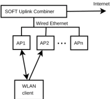
AP1 AP2 APn SOFT Uplink Combiner
WLAN client
Wired Ethernet
Internet
...
Figure 1: SOFT’s System Architecture. On the
up-link, multiple APs may hear the transmission of the wiless client. They communicate their confidence in the re-ceived bits to the SOFT Combiner. SOFT combines their information to reconstruct a clean packet from multiple faulty receptions.
For simplicity, we describe our ideas within the con-text of binary modulation, where a symbol refers to one bit. Our algorithm and lemmas can be easily ex-tended to other modulation schemes, as discussed in the appendix.
2.1 An Interface that Returns Soft Values
SOFT sits below the MAC, between the physical layer and the data link layer. It modifies the inter-face between the two layers. Instead of returning 0’s and 1’s, the physical layer returns for each bit a real number, which we call a soft value (SV). The SV gives us an estimate of how confident the physical layer is about the decoded bit. The decoded bit is zero when the corresponding SV is negative, and is one otherwise. The smaller the absolute value of the soft value, the less confident the physical layer is in whether the sent bit is 0 or 1. Note that regardless of the modulation scheme, the physical layer always first computes a soft-value, which it then decodes to “1” or “0” depending on the sign of the soft value. Traditionally, the SV has been hidden from the higher layers. However, in SOFT, the physical layer exposes a normalized version of this soft value to the data link layer.
SOFT associates soft values with each bit, we refer to this replacement of bits with their corresponding soft values as a soft packet or s-packet. The data link layer in SOFT decodes such s-packets to obtain the trans-mitted packets. Except for some details, the decoding algorithm is similar for the uplink and the downlink scenarios.
While the current design of SOFT targets WLANs, including 802.11a/b/g, we believe that our ideas ap-ply to Ultra Wide Band (UWB) and WiMax LANs. Although the details of the physical layer differ across technologies and within the same technology, all phys-ical layer design can easily expose an SV for each de-coded bit/symbol. Generally speaking, the function of a wireless receiver is to map a received signal to the
symbol that was transmitted. To do so, the receiver computes a soft value from the received signal for each symbol, which is a real number that gives an estimate of the transmitted symbol. The receiver then maps the soft value to the symbol which is closest to it. For ex-ample when the symbols correspond to “0” or “1” bit, the soft value is decoded to a “1” bit if it is positive and “0” otherwise. The soft value can be easily gen-eralized to systems where each symbol represent more than one bit.
2.2 Uplink
Figure 1 shows the SOFT architecture on the uplink. It is designed to exploit spatial diversity through the cooperation of several access points. Each AP in the WLAN infrastructure offers a different communication channel to the client. We leverage the comparatively high bandwidth of the wired Ethernet connecting the access points. Each AP forwards all s-packets including those that are corrupted to the combining agent. The combining agent is a logical module, that may reside on one of the access points or on a different machine on the local Ethernet, and can be thought of as an uber-access point.
The combining agent does not run the decoding for packets that are already correctly received, as deter-mined by the checksum. It invokes the packet combin-ing procedure only for corrupted packets. The agent first needs to identify the set of s-packets (received at different APs) that correspond to the same transmis-sion. To do this, it decodes the header of each s-packet to determine the packet-id of the transmitted packet. Packet-id is a pseudo random sequence assigned by the transmitter to each packet and maintained across retransmissions. S-packets having the same packet-id correspond to receptions of the same packet or its re-transmission at different APs. The combining agent keeps this set of packets corresponding to the same transmission in a hash table that is keyed by the packet-id. Headers, which include the packet-id, are en-coded with a lot of redundancy, hence they are highly likely to be received with no errors. Packet-ids are therefore assumed to be received with little error.
The next step for the combining agent is decoding. When an s-packet arrives at the agent, we face one of two situations: 1) The arriving packet is uncorrupted, i.e., it passes the checksum. In this case, the packet is forwarded toward its IP destination and other packets with the same packet-id are dropped. 2) The packet is corrupted, in which case all the packets with the same packet-id are passed to the combining algorithm (described in §3, to attempt to correct the faulty bits. If the combining algorithm succeeds, the correct packet is forwarded and the packets are deleted from the hash table. If the combining algorithm fails, the agent waits for new soft-packets with the same packet-id.
We note that the combining agent keeps a hash ta-ble of packet-ids for recently forwarded packets. When a new packet arrives, the agent checks the table to see whether a packet with a similar id has been cor-rectly forwarded, in which case the new packet is ig-nored. This eliminates redundant forwarding. Finally, old soft-packets that were never recovered are dropped after a timeout.
2.3 DownLink
SOFT’s design for the downlink exploits time diver-sity. Faulty s-packets are stored and combined with later retransmissions to increase the overall potential of recovery. The process of combining multiple faulty transmissions to correct bit errors is similar to that of combining s-packets across APs, except that the com-bining agent in the case of the downlink runs on the client node itself.
2.4 ACKs & Retransmissions in SOFT
SOFT modifies the transmitter and receiver mod-ules. If a SOFT receiver has the intended next-hop MAC address, it immediately acks correctly received packets using 802.11 synchronous acks. For each 802.11 ack-ed packet, the receiver communicates the correct reception to the combining agent to allow it to discard the s-packets corresponding to the ack-ed packet. On the other hand, if the packet is faulty or if the receiver is not the intended next-hop, it communicates the s-packet to the combining agent. The agent stores faulty receptions and uses them to reconstruct a clean version of the packet as described above. If the reconstruction succeeds, the agent sends an asynchronous ack to the sender with the packet-id. The lack of an ack causes the sender to timeout and retransmit the packet.
After transmitting a packet, the SOFT sender waits for an ack. If it receives a synchronous 802.11 ack, it moves on to the next packet waiting transmission. Oth-erwise, the packet may need to be retransmitted which happens when the combining agent at the receiver fails to recover a clean copy. The retransmission strategy varies between the uplink and downlink.
In the case of the uplink, SOFT disables link-layer retransmissions to allow the combining agent enough time to recover packets that the APs receive in error. Specifically, since cooperation requires the APs to com-municate over the wired LAN, it is not possible to re-cover a corrupted packet within the time limit for send-ing a synchronous 802.11 ack. Thus, SOFT WLANs operate in 802.11’s unicast mode but with no retrials. The SOFT sender stores unack-ed packets in a hash table keyed on the packet-id. Whenever it receives an asynchronous ack, it looks up the ack-ed packet-id in its table, removes the corresponding packet, and reset any scheduled retransmissions for that packet. Unack-ed packets are pending for retransmission, unless they
are ack-ed within a retransmit interval. The value of the retransmit interval depends on the wireless technology and the bit rate. It should take into ac-count the communication time between the APs and the combining agent over the wired LAN, the time to retransmit an asynchronous ack over the WLAN, and any potential congestion. We estimate this time using an exponentially moving average in a manner similar to the TCP RTT estimate. The retransmit interval is set to the average estimate plus one standard devi-ation.
On the downlink, the retransmission strategy can be simplified since packet recovery does not involve any communication between nodes. In particular, we envi-sion that SOFT will be implemented in hardware on the wireless card itself. In this case, we believe SOFT can check whether a packet is recoverable via combin-ing with prior receptions very quickly.2
The combining algorithm can be executed within a SIFS (i.e., 28 mi-croseconds), and the receiver can immediately send an 802.11 ack if it is able to reconstruct the packet. Thus, the transmitter on an AP can use the current strategy for retransmission and expects acks to be in-order.
3
Combining Algorithm
How should one combine the information from mul-tiple corrupted receptions in order to maximize the chances of recovering a clean packet? For both uplink and downlink, the combining algorithm is presented with multiple s-packets that correspond to the same original transmission. None of these s-packets is suffi-cient on its own to recover the original transmission. Yet, because these are s-packets, they carry SVs for each bit, which give the combining algorithm a hint about the noise level in that bit.
Say that the combiner is presented with 3 s-packets. Recall that a positive SV means “1”, a negative SV means “0”, and that the magnitude of the SV refers to the PHY’s confidence in the decision. Let the SV cor-responding to bit i in these s-packets take the values: 0.3, −0.1 and −0.2. How does the combining algorithm decide whether bit i is “0” or ”1”?
The most straightforward approach would take the maximum corresponding SV since it is the reception with most confidence. Thus, in the above example, one would say that bit i is a “1” because the reception with the highest confidence (i.e., 0.3) has mapped it to “1”. But is this the optimal answer? Clearly there are other approaches that look equally correct. For example, one
2
Our combining algorithm in §3 uses a weighted sum of the s-packets. Thus, there is no need to keep all s-s-packets. The sum can be constructed incrementally as more receptions arrive. Combin-ing requires only combinCombin-ing the most recently received s-packet with the weighted sum of prior s-packets, which can be quite fast. Thus, the card needs not maintain more than an s-packet worth of memory.
may resort to a majority vote. In this case, two recep-tions map this packet to “0” (−0.15 and −0.2) whereas one reception maps it to “1” (one positive value of 0.3). Thus, a majority voting approach would decide that the bit should be “0”, which is the opposite of the previous approach.
There are other approaches too, such as comparing the sum of the positive values to the sum of the nega-tive values, or comparing the sum of the squares of the positive values to the sum of the squares of the nega-tive values, etc. We would like to pick the combining strategy that maximizes the recovery probability.
In SOFT, we analyze the packet recovery probabil-ity and adopt a combining strategy that is provably optimal. Our strategy uses the sum of SVs weighted by the noise variance at their corresponding AP. It is based on the following lemma, which gives the optimal decision for an additive Gaussian white noise channel (AGWN), a typical model for indoor wireless chan-nels [23].
Lemma 3.1. Let y1, . . . , yk be SVs that correspond
to multiple receptions of the same bit over different AWGN channels. To maximize the recovery probabil-ity, one should map the bit to “0” or “1” according to the following rule:
if X
i
yi
σ2 i
≥0 then the bit is “1”, otherwise it is a “0”, where σ2
i is the noise variance in the ith AWGN
chan-nel.
The proof of the lemma is in the appendix. We also note that though the above lemma focuses on modu-lation systems where a symbol is a single bit, the ap-pendix shows a generalized form that applies to larger symbol size.
We note a few interesting points.
• Straightforward approaches for combining multiple receptions including taking the SV with the highest confidence or doing a majority vote are suboptimal. • One should not treat all receptions equally. This is particularly important for the uplink where different receptions traverse a significantly different wireless channel. For example, the wireless transmitter might have a line of sight to one of the access points, re-sulting in lower noise variability in this channel, and thus one should trust this channel more. One should not think that the more receptions she/he has the lower the error will be. Including physical informa-tion from APs with highly variable channels (i.e., large σ2
) without accounting for that variability de-creases the overall performance.
• The decision rule above requires the noise variance, σ2
i, on each channel. We compute this value by
look-ing at the variance in the received signal, as ex-plained in §5.
• Since the result in Lemma 3.1 assumes AWGN chan-nels, it is natural to wonder how closely real indoor wireless signals match the result in lemma 3.1. Ex-perimental results in §8 show that the decision strat-egy advocated by Lemma 3.1 is superior to other strategies in practice.
4
Direct Sequence Spread Spectrum
802.11b networks use Direct Sequence Spread Spec-trum (DSSS). DSSS trades off high bit rate for im-proved error resilience. Specifically, each bit is mapped to a multi-bit codeword before transmission. A simpli-fiedDSSS example may map a “1” bit to the codeword 11111111 and “0” to 00000000. This reduces efficiency as the sender has to transmit many more bits for each logical bit, but it significantly improves resilience be-cause an error has to change at least 4 bits in a code-words before it causes an error in mapping a received codeword to the correct logical bit. The length and val-ues of the codewords used in 802.11b vary depending on the bit rate.
The combining algorithm described in §3 can be ap-plied to 802.11a/b/g [14]. In this case, the combining algorithm is used to decode individual bits. DSSS de-coding is applied on sequences of these decoded bits to decode codewords and map them back to logical bits. Specifically, the receiver computes the Hamming dis-tance between a received codeword and possible code-words, and maps the received codeword to the logical bit that minimizes the Hamming distance [11].
We can however do better. We can exploit the fact that only a few codewords are allowed in 802.11b to further improve the performance. Thus, instead of mapping each bit in isolation as we did in lemma 3.1, we map each sequence of SVs to either a zero-codeword or a one-codeword. Say that we have k s-packets cor-responding to the same data packet. Let us focus on the ith codeword in these s-packets. Let each
word contain m bits. In this context, a soft code-word (s-codecode-word) is a sequence of m SVs, i.e., ~yi =
(y1, y2, . . . , ym). The following lemma gives the
opti-mal combining strategy for the case of AWGN chan-nels, typically used in analyzing indoor wireless.
Lemma 4.1. Let ~y1, . . . , ~yk be multiple s-codewords
that correspond to the same codeword transmitted over different AWGN channels. Let x~1 = (x1
1, . . . , x 1 m) be
the codeword corresponding to logical “1” and x~0 =
(x0 1, . . . , x
0
m) the codeword corresponding to a logical
“0”. The following strategy maximizes the recovery probability: if k X i m X j yij(xj1− x 0 j) σ2 i ≥0, then “1”, otherwise “0”, where σ2
i is the variance in the i
th AWGN channel. 0 0.1 0.2 0.3 0.4 0.5 0.6 0.7 0.8 0.9 1 -1 -0.5 0 0.5 1
Fraction of Soft Values
Soft Values SVs
Figure 2: Soft Value Distribution:A typical
distribu-tion of the soft values seen in our testbed. The two modes correspond to “0” and “1” bits.
The proof of the above lemma is in the appendix.
5
Estimating the Noise Variance
In order to compare the soft values observed at dif-ferent receivers, we require the corresponding σ2
i of the
channels. SOFT estimates a channel’s variance exper-imentally using the empirical distribution of the SVs. For the ith AWGN channel, the SV value of a bit can
be expressed as
yi = x + ni,
where ni is a white Gaussian noise and x is the
trans-mitted bit value ( x = −1 for a “0” bit and x = +1 for a“1” bit). Thus, conditioned on the bit value, yi is
also a Gaussian variable with the same variance as ni.
Thus, we estimate the variance in ni using the variance
in the yi’s. Figure 2 shows the soft values distribution
(i.e., the yi’s) at a particular AP in our testbed.
Note that the soft values have the same distribution as the ni’s only when we fix the value of the
transmit-ted bit (i.e., a fixed x in the equation above). In general we cannot tell for sure at an AP which received SV cor-responds to a “0” and which corcor-responds to a “1”. But because the vast majority of soft values already corre-spond to correctly decodable bits, the statistical vari-ance of the absolute value of the soft values is a good estimate for σ2
i. We compute this for every packet by
using all the soft values from it.
The above assumes that the channel noise variance stays the same. One however can enhance the estimate by using an exponential decaying average over a few packets recently received from the same sender.
6
Reducing Overhead
In the uplink case, SOFT transfers the s-packets from the APs to the combining agent over the wired Ethernet. We leverage the much higher wired Ether-net bandwidth to improve the scarce wireless through-put. The increase in the consumed Ethernet band-width however is an overhead of the system. We note that in a typical operation environment (e.g., univer-sity campus), Ethernet throughput is an order of mag-nitude larger than WLAN throughput. Furthermore,
though wireless throughput is increasing at a steady speed, it is likely that the difference between Ethernet and WLAN throughput will continue to hold; 10 Gb/s Ethernet (10GbE) is already on the market and 100 Gb/s Ethernet (100GbE) is presently under develop-ment by the IEEE [1].
Despite the big difference between Ethernet’s and WLAN’s throughput, it is important to keep SOFT’s overhead bounded. The wired bandwidth consumed by transferring s-packets depends on how we express an SV. If an SV is expressed as an 16-bit number, then each packet will be amplified 16 times. To reduce the overhead, we need to quantize the SVs. Optimal quan-tization depends on the σ2
of the channel. That is, for a particular distribution of SVs, one needs to integrate the total area and divide into 2k bins where k is the
number of bits used to express each SV. In practice, however, we found that a uniform quantization works equally well.
Thus, our quantization algorithm works as follows. It picks a constant cutoff for all SVs across all exper-iments. The cutoff value depends on the modulation scheme and thus should be calibrated for each 802.11 bit rate. Values above the cutoff are reduced to the cut-off value. Every SV is expressed using 3 bits, one for the sign and 2 bits for the magnitude. Though this still consumes Ethernet bandwidth, it keeps the overhead within practical limits.
7
Implementation
7.1 Hardware and Software Environment
We have implemented a prototype of SOFT using Software Defined Radios (SDR). SDRs implement all the signal processing components (source coding, mod-ulation, clock recovery, etc.) of a wireless communi-cation system entirely in software. The hardware is a simple radio frequency (RF) frontend, which acts as an interface to the wireless channel. The RF frontend con-verts the signal generated by the SDR from digital to analog and transmits it on the wireless channel. At the receiver, the base-band signal is converted from ana-log to digital and passed to the SDR software. Thus, SDRs expose the raw signal to software manipulation and thus present an opportunity to exploit information traditionally available only at the physical layer.
We use the Universal Software Radio Peripheral (USRP) [15] as our RF frontend. USRP is a generic RF frontend developed specifically for the GNU Radio SDR. The software for the signal processing blocks is from the open source GNURadio project [7].
7.2 Implementation Details
We export a network interface to the user, which can be treated like any other network device (e.g., eth0). On the sending side, the network interface pushes the
Mueller & Muller Timing Recovery Match Filter h[n] Slicer (Decision Device) > < 0
...
decoded bits match valuesFigure 3:The block diagram of the different components in the receiver module. The match values output by the match filter in the figure correspond to the soft values used in our algorithms.
packets to the GNU software blocks with no modifica-tions. On the receiving side, the packet is detected and demodulated. We use the output of the match filter as our SVs as described in §2.1. This value is a 32-bit float, which we quantize according to the algorithm in §6, and pass to SOFT. Our SOFT implementation matches the description in §2.
The modulation scheme we use in our implementa-tion is Gaussian Minimum Shift Keying (GMSK ). But the ideas we develop in this paper are applicable to any modulation scheme. The main reason for using GMSK here is that the GNU radio project has a mature GMSK implementation. Currently, GNU implementa-tions of other modulation techniques are either non-existent of buggy. GMSK is a form of Phase-Shift Key-ing (PSK) which is widely used in modern communi-cation systems. For example, GSM, a widely used cell-phone standard, uses GMSK, and 802.11 uses Binary and Quadrature Phase Shift Keying (BPSK/QPSK). GMSK has very good bit-error properties, has a sim-ple demodulation algorithm and excellent spectral ef-ficiency.
Fig. 3 shows the block diagram of the components in our receiver. The signal is first passed through a clock recovery module, which ensures that the opti-mum sampling time is found. The output of the clock recovery is passed through a matched filter which out-puts the soft value we use in our algorithms. Soft value computation depends on the modulation scheme used. But the basic intuition behind all matched filters is the same. They integrate the received signal energy so that the zero-mean gaussian noise is cancelled out and output a single float value which is the soft value. This soft value is now passed to a decision device that esti-mates what bit was transmitted depending on the sign of the soft value.
The soft value gives us a way to compute the confi-dence in the bit estimated by the decision device. We combine the soft value along with the corresponded es-timated bits to form a soft-packet. The soft-packet is now passed to the combining agent through the wired ethernet.
8
Experimental Results
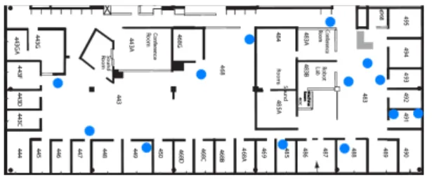
We evaluate SOFT in a 13-node software radio testbed. The topology is shown in Figure 4. Each node is a commodity PC connected to a USRP GNU
ra-Figure 4: Testbed Topology.The figure shows the test-ing environment. The dots mark the locations of the GNU-Radio nodes.
dio [15]. The USRP connects to the PC via USB 2.0. Thus, its throughput is limited to 32MB/s. This also limits the bandwidth of the signal to at most 4MHz, which is enough for performing representative narrow-band experiments.
SOFT’s combining algorithm works the same whether the s-packets are the result of overhearing at multiple APs or retransmissions at a single wireless receiver. Thus, we use the uplink experiments to ex-plore the various aspects of SOFT and its combining strategy and revert to the downlink experiments to in-vestigate retransmissions under SOFT. In general, the uplink also combines faulty s-packets with their poten-tially faulty retransmissions to recover a clean packet. Our experiments however deactivate combining with retransmissions for the uplink to disentangle the gains due to space diversity from those due to time diversity.
8.1 Setup
In each experiment, we pick three nodes as our access points (APs), and randomly vary the sender among the nodes in the testbed. Each randomly chosen sender transmits 500 packets, where packet size is 1500B. One of the three APs in each experiment is designated as the master AP and runs the combining agent. The other APs send their s-packets to the master AP over the wired Ethernet, which combines information across s-packets to reconstruct a clean packet. In uplink ex-periments, retransmissions are turned off to separate gains due to space diversity from those caused by time diversity.
For the downlink experiments, we randomly pick a sender-receiver pair and transfer 500 packets between them. Here, we focus on the gains due to time diversity, i.e., reductions in loss rate due to SOFT’s ability to re-cover clean packets by combining faulty transmissions with faulty retransmissions of the same packet.
It should be noted that because GNU Radios per-form all processing in software, many of the timing details of 802.11 cannot be implemented. This has two implications for our setup. In particular, unless one changes the FPGA code, one cannot consistently send synchronous 802.11 acks on time. We emulate 802.11 acks by sending the ack packet immediately after the
data packet, as fast as the SDR system permits. Sec-ond, with no proper timing control, one cannot imple-ment 802.11’s backoff algorithm. Thus, we do not have a mechanism to avoid collisions. Since we run only one sender at any time, our senders do not collide with each other. They may however be affected by interfer-ing signals in the same band. We try to run our exper-iments at night when wireless activities in our lab are limited. Note that although the errors resulting from interfering signals reduce the delivery rates, they do not bias the results towards any particular protocol, among those compared. The compared protocols pro-cess the same reception data, each with its approach for recovering correct packets.
8.2 Compared Approaches
We compare the following approaches
• SOFT: This approach adopts the architecture in §2 and uses the combining strategies of Lemmas 3.1 and 4.1.
• MAX Confidence: This is similar to SOFT but
with a max-confidence combine strategy. Specifi-cally, when combining multiple SVs that correspond to the same bit, the bit is mapped to “0” or “1” ac-cording to the SV with the maximum absolute value. • Majority Vote: This is also similar to SOFT but it uses a majority vote to combine multiple receptions. Specifically, each bit is assigned the value agreed on by the majority of the receptions (i.e., the majority of the APs).
• Current Approach: This approach is similar to
the current WLAN scenario which does not allow the APs to cooperate, and does not combine bits across different receptions.
• MRD: This is a prior cooperative scheme for packet recovery [19]. MRD does not use physical layer in-formation. It works as follows. It divides each packet into blocks. For each block, it assumes that at least one of the APs has correctly received the bit values for that block. It attempts to recover a faulty packet by trying every version received for each block, and checking whether such combined packet passes the checksum. MRD computational cost is exponential in the number of blocks. Thus, in order to be compu-tationally feasible, MRD recommends using 6 blocks per packet [19], which is what we use in our experi-ments.
8.3 Metrics
We use the following metrics:
• Packet Delivery Rate: This is the fraction of trans-mitted packets that the WLAN correctly delivers to the destination. For the current approach, the deliv-ery rate is computed as the fraction of uncorrupted packets received at the best AP, i.e., the one with the
0 0.2 0.4 0.6 0.8 1 0 0.2 0.4 0.6 0.8 1
Cumulative Fraction of Runs
Packet Delivery Rate
Current Approach MRD SOFT
Figure 5: CDF of Packet Delivery Rates.SOFT
sig-nificantly improves the packet delivery rate. While the mean delivery rate in the current approach and MRD is less than 7%, the mean SOFT delivery rate is as high as 62%. Retransmissions are turned off in these experiments, thus the improvement in delivery rate is mainly due to the use of soft values and the effect of spatial diversity.
lowest loss rate for the particular sender. For coop-erative approaches, the delivery rate is the fraction of packets that were successful recovered either im-mediately at the radio receiver, or after running the combining algorithm. The delivery rate is compute for all approaches without retransmissions.
• Number of Retransmissions: This is the number of times the sender had to retransmit the same packet to ensure errorless delivery to higher layer. Retrans-missions are activated only during downlink experi-ments. As such, the uplink experiments serve to eval-uate the gains due to spatial diversity gains. The downlink experiments, where no spatial diversity ex-ists, are used to evaluate the time diversity gains.
8.4 Importance of Cooperation & Soft Values
We are interested in quantifying the impact of co-operation on the reliability of WLANs. In particular, how much improvement in loss rate should one expect from combining packets across APs? Further, is there a significant benefit for obtaining physical layer informa-tion or a higher-layer technique like MRD is sufficient? To answer these questions we perform 100 runs of the experiment described in §8.1. Specifically, each time we pick three APs from the nodes in the testbed and a random sender, which transmits 500 packets. We com-pute the packet delivery rate for SOFT, the current approach, and MRD (with 6 blocks per packet). Fig-ure 5 compares the CDFs of the deliver rates for the three schemes.
The figure shows the importance of using soft values in cooperative recovery. The mean delivery rate in the current approach is less than 7%. MRD does not help much when delivery rates are considerably low. Such environments are highly lossy, while MRD can recover only from a handful of bit errors. In contrast, SOFT’s mean delivery rate is 62%, which is about an order of magnitude better than both the current approach and
0 0.2 0.4 0.6 0.8 1 0 50 100 150 200 250
Packet Delivery Rate
Number of Blocks Allocated
MRD SOFT
Figure 6: Comparing Delivery Rates for Increased MRD Blocks.Figure plots the delivery rate of one sender as a function of increased MRD blocks. SOFT’s delivery rate for this sender is about 78%. MRD cannot match SOFT’s performance even with hundreds of blocks. In prac-tice, it is infeasible to have such many blocks both because of computational overhead and the checksum losing its er-ror detection capability.
MRD.
We also check whether having a larger number of blocks improves MRD’s performance. Thus, in Fig-ure 6, we focus on a specific sender and a specific AP set. We vary the number of blocks used by MRD. Note that MRD’s computational complexity increases expo-nentially with the number of blocks. Computing the CRC for a large number of blocks is infeasible in prac-tice. But since we know the transmitted packet con-tent, we can check whether MRD recovers a correct packet without incurring the exponential cost. To do so, we compare the received blocks directly against the transmitted ones. Such a check is however infeasible in practical situations since the APs do not know a priori the sent data. Figure 6 shows that even if it would be practical to increase the number of MRD blocks to 200, SOFT still does better. This result further emphasizes the importance of exposing the information available to the physical layer to higher layers.
8.5 The Role of the Combining Rule
We also want to investigate how the delivery rate changes with the strategy used to recover packets from multiple soft copies. In particular, Lemma 3.1 advo-cates using a weighted sum of the SVs. But the lemma makes this assertion based on a AWGN model of the channel. Would the result of this lemma hold in prac-tice?
Figure 7 compares the CDFs of packet delivery rates for various combining rules. The experiments are run using the setup described in §8.1 and the CDFs are computed over all such runs. The figure shows that SOFT’s weighted-sum strategy performs better than taking a majority vote or using the bit value with the maximum confidence. Thus, the experimental results support the analysis in §3.
It is also interesting to note that a majority vote works better than trusting the largest SV. This is
0 0.2 0.4 0.6 0.8 1 0 0.2 0.4 0.6 0.8 1
Cumulative Fraction of Runs
Packet Delivery Rate
Max Conf Majority SOFT
Figure 7: CDFs of Delivery Rates for Different
Combining Strategies. The figure compares the
deliv-ery rate under three combining strategies: SOFT, Max-Confidence, and Majority-Vote. It shows that SOFT’s weighted-sum strategy performs significantly better than the others, which supports our analytical results.
ticularly true at low delivery rates. In this case, all APs are receiving very poor signals. The differences in their SVs are close to the noise level. Taking the max SV allows a biased SV to deviate the results, whereas taking a majority vote increases resilience.
8.6 Impact of Noise Variance
Our analysis highlights the importance of account-ing for the noise variance when combinaccount-ing SVs received from different APs. Here, we experimentally check how normalizing by the noise variance affects delivery rates. The noise variance is computed at each AP experimen-tally using its received data, as described in §5.
Figure 8 shows that accounting for the noise vari-ance can improve the delivery rate by about 14%. It is interesting to note that the noise variance is particu-larly important when the delivery rates are neither too low nor too high. This is because at very low delivery rates, all APs have highly noisy channels such that the difference in their noise level does not matter. At very high delivery rates at least one and sometimes two APs have very good channels and can still recover the sig-nal despite the bias introduced by the more challenged AP. It is at moderate delivery rates when a biased AP produces destructive effect, polluting the SVs of the two not very confident APs.
8.7 Direct Sequence Spread Spectrum
This section shows that SOFT’s benefits extend to scenarios with direct sequence spread spectrum (DSSS). We repeat the experiments described in §8.1 with DSSS. We compare SOFT’s delivery rates with the delivery rates of the current approach. As ex-plained earlier DSSS improves packet delivery at the cost of using lower bit rate for the same bandwidth.
In comparison with Figure 5, Figure 9 shows a sig-nificant improvement in the overall loss rate for both SOFT and the current approach. SOFT, however, still significantly outperforms the current approach. With
0 0.2 0.4 0.6 0.8 1 0 0.2 0.4 0.6 0.8 1
Cumulative Fraction of Runs
Packet Delivery Rate
SOFT with no Weights SOFT
Figure 8: CDF of Delivery Rates with and
with-out Normalization by the Noise Variance. The
fig-ure shows that normalizing the SVs by the noise variance improves the delivery rates, and that the normalization is particularly important for moderate to moderately-high delivery rates. 0 0.2 0.4 0.6 0.8 1 0 0.2 0.4 0.6 0.8 1
Cumulative Fraction of Runs
Packet Delivery Rate Current Approach
SOFT
Figure 9: CDFs of Delivery Rates under DSSS.The
figure shows that DSSS improves the delivery rates for both SOFT and the current approach. For these environments, SOFT eliminates all losses for the vast majority of the runs.
SOFT, 97% of all runs experience perfect delivery rates, as opposed to only 72% with the current ap-proach. Thus, for environments with moderate to high delivery rates, SOFT eliminates most of the residual losses.
8.8 Retransmissions on the Downlink
We also evaluate SOFT’s performance on the down-link. In this case, SOFT reconstructs a faulty packet by combining multiple receptions at the same receiver. We want to compute the number of retransmissions required to recover a correct packet, with and with-out SOFT. We perform the following experiment. We pick a random sender-receiver pair from the nodes in testbed. The sender transmits 500 different packets. In contrast, to prior experiments, the sender retransmits every packet until the receiver recovers a correct copy of the packet. We repeat the same experiment for 30 sender receiver pairs.
Figure 10 shows a CDF of the number of retransmis-sions per packet, taken over all packets and all sender-receiver pairs. The figure shows that in our testbed, only 33% of the packets on the downlink are received with no need for retransmission (the value for #Re-transmissions = 0). SOFT cannot improve this number on the downlink because there is no cooperation. But
0 0.2 0.4 0.6 0.8 1 0 5 10 15 20 25 30 Fraction of Packets Number of Retransmissions Current Approach SOFT Recombination
Figure 10: CDFs of the Number of Retransmissions
on the Downlink. SOFT correctly recovers 94% of the
packets with less than one retransmission. The current ap-proach needs up to 18 retransmissions to achieve the same delivery rate. Magnitude Cutoff 0.2 0.4 0.6 0.8 1 Fraction of Packets 0 0.1 0.2 0.3 0.4 0.5 0.6 0.7 0.8
2 Bits 3 Bits Float
Figure 11: Impact of Quantization on the Delivery Rates.The figure shows two results: 1) It is sufficient to use 3 bits to express the value of the SVs. 2) the quantiza-tion is fairly resilient to the choice of cutoff value.
SOFT significantly improves the overall performance of the downlink. In particular, 94% of the packets are correctly received after one retransmission. In contrast, the current approach needs up to 18 retransmissions to achieve the same reliability.
8.9 Impact of Quantization
To reduce the overhead over the wired Ethernet, we quantize the SV values and express then using only 3 bits. We want to ensure that by doing so we are not loosing too much in term of delivery rates. Thus, we plot the average delivery rate of 30 random runs for various quantization parameters.
Figure 11 shows two important results. First, our approach is fairly resilient to the choice of the cutoff for values in the rage [0.4, 0.8]. Thus, despite that the SVs collected at different APs have different variance (i.e., spread), we can still use the same cutoff value across all APs. Second, it is sufficient to express the SVs using 3 bits, one for the sign and two bits for the magnitude. This reduces the size of an s-packet and significantly reduces the wired overhead.
9
Related Work
Related work falls in two areas.
(a) Cooperative Design Spatial cooperation, i.e., combining information from multiple nodes to boost throughput, has been discussed within recent work [9, 17, 22]. Most of the work in this area is theoretical with no system implementation or experimental re-sults. The main difficulty in implementing the theo-retical proposals is their reliance on tight synchroniza-tion across nodes. Some prior work [18, 24] advocates combining frames received from adjacent access points to improve uplink WLAN performance, but they are both based on simulation and ignore protocol level is-sues such as ARQ. Experimental work on spatial coop-eration either assumes multiple antennas on the same node (i.e., MIMO systems) [23] or does not use physi-cal layer information [19, 6]. In comparison, this paper presents a practical protocol that integrates spatial co-operation with physical-layer information and does not assume MIMO nodes.
The closest work to ours is by Miu et al. [19], who propose combining receptions from multiple access points to recover faulty packets. Their work does not use physical layer information. It divides the packet into multiple blocks. When the access points receive conflicting blocks, this proposal attempts to resolve the conflict by trying all block combinations and checking whether any of the resulting combinations produces a packet that passes the checksum. The overhead of their approach is exponential in the number of erroneous blocks and thus too costly when there is significant loss. Our experimental results in §8.4 compare against their approach and demonstrate the importance of us-ing physical layer information.
(b) Soft Decoding The use of physical layer informa-tion in decoding is usually referred to as soft decoding. Prior theoretical work has discussed soft decoding and applied it to various codes including Reed Solomon and LDPC [12, 10, 25]. The Viterbi decoding algo-rithm has a soft extension (SOVA) that includes phys-ical information as a priori probabilities of the input symbols [13]. Also, some prior work has suggested that a receiver should save a corrupted packet and combine it with a later retransmission [8, 2]. Our work builds on this foundation but differs in two main ways. First, prior work studied a single wireless channel, whereas we present a network architecture that combines soft information from multiple APs in a cooperative de-sign. Second, we focus on practical networking issues and present a working implementation of our design.
Concurrently to our work, a second research group was looking at passing physical layer hints to higher layers [16]. The two projects were developed indepen-dently and each group learned about the other’s re-search only after most of the ideas were developed. In
particular, our ideas as well as our initial results have been documented in a class report that was submitted as early as November 2006. The two projects use soft information but the ideas differ considerably. The work in [16] uses a threshold over soft information. When the soft information associated with a received codeword is above the threshold, the codeword is considered to be goodand when it is below the threshold the codeword is bad. The threshold is updated dynamically based on prior observations. The work in [16] propose to use this threshold with a postamble to discover which chunks in a packet are received incorrectly, and retransmit them. In contrast to the above, our project does not use a threshold. It recovers erroneous packets by combining soft information across multiple erroneous receptions. Also, in contrast to [16], our work combines soft infor-mation from receptions at different receivers, in which case it also adjusts for channel variance. Finally, our work leverages the high Ethernet bandwidth between access points in WLAN to perform soft information combing.
10
Conclusion
Today’s wireless networks have largely adopted the abstractions of wired networks, despite the fact that they come with unique challenges. Lossy links and poor connectivity are two main problems in wireless networks that have direct impact on application per-formance and user satisfaction. Current approaches to address these problems have mostly been inadequate. However, wireless media provide intrinsic resilience due to their spatial and temporal diversity, and this presents opportunities to address their challenges with novel solutions.
Computer networks have traditionally been designed with narrow interfaces between layers in the stack. In this paper, we have presented SOFT, a scheme that increases the reliability of wireless networks by adopt-ing a more informative interface between the physical and higher layers, and using confidence values from the physical layer to cooperatively reconstruct packets at the data layer. Our experimental results demonstrate that SOFT improves the mean packet delivery rate and reduces the required number of retransmissions by an order of magnitude.
References
[1] 100 Gigabit Ethernet Transmission Sets New Record, 2006.
http://arstechnica.com/news.ars/post/20061115-8231.html.
[2] T. W. A. Avudainayagam, J.M. Shea and L. Xin. Reliability Exchange Schemes for Iterative Packet Combining in Distributed Arrays. In Proc. of the IEEE WCNC, volume 2, pages 832 – 837, 2003. [3] A. J. Nicholson and Y. Chawathe and M. Y. Chen
and B. D. Noble and D. Wetherall. Improved Access Point Selection. In MobiSys, 2006.
[4] D. Aguayo, J. Bicket, S. Biswas, G. Judd, and R. Morris. Link-level Measurements from an 802.11b Mesh Network. In SIGCOMM, 2004.
[5] P. Bahl, J. Padhye, L. Ravindranath, M. Singh, A. Wolman, and B. Zill. DAIR: A Framework for Managing Enterprise Wireless Networks Using Desktop Infrastructure. In Hotnets, 2005.
[6] S. Biswas and R. Morris. Opportunistic Routing in Multi-Hop Wireless Networks. In SIGCOMM, 2005. [7] E. Blossom. GNU Software Defined Radio.
http://www.gnu.org/software/gnuradio, 2006. [8] S. S. Chakraborty, E. Yli-Juuti, and M. Liinaharja.
An ARQ Scheme with Packet Combining. IEEE Communication Letters, 1998.
[9] S. Diggavi, N. Al-Dhahir, A. Stamoulis, and A. Calederbank. Great Expectations: The Value of Spatial Diversity in Wireless Networks. Proceedings of the IEEE, 92(2):219 – 270, Feb. 2004.
[10] R. Gallagher. Low-Density Parity-Check Codes. MIT Press, Cambridge, MA, 1963.
[11] A. Goldsmith. Wireless Communications. Cambridge University Press, 2005.
[12] V. Guruswami and M. Sudan. Reflections on Improved Decoding of Reed-Solomon and Algebraic-Geometric Codes. IEEE Information Theory Society Newsletter, 52(1):6–12, 2002. [13] J. Hagenauer and P. Hoecher. A Viterbi Algorithm
with Soft-Decision Outputs and its Applications. In IEEE GLOBECOM, 1989.
[14] p. a. IEEE 802.11 WG. Wireless lan medium access control (mac) and physical layer (phy) specifications, 1999.
http://standards.ieee.org/getieee802/802.11.html. [15] E. Inc. Universal software radio peripheral.
http://ettus.com.
[16] K. Jamieson and H. Balakrishnan. PPR: Partial Packet Recovery for Wireless Networks. Technical report, MIT, 2007.
[17] J. Laneman, D. Tse, and G. Wornell. Cooperative diversity in wireless networks: Efficient protocols and outage behavior. IEEE Transactions on Information Theory, 50(12), 2004.
[18] V. Leung and A. Au. A wireless local area network employing distributed radio bridges. Wireless Networks 2, pages 97–107, 1996.
[19] A. K. Miu, H. Balakrishnan, and C. E. Koksal. Improving Loss Resilience with Multi-Radio Diversity in Wireless Networks. In 11th ACM MOBICOM Conference, Cologne, Germany, Sept. 2005.
[20] C. Reis, R. Mahajan, M. Rodrig, D. Wetherall, and J. Zahorjan. Measurement-Based Models of Delivery and Interference. In SIGCOMM, 2006.
[21] M. Rodrig, C. Reis, R. Mahajan, D. Wetherall, and J. Zahorjan. Measurement-based characterization of 802.11 in a hotspot setting. In ACM SIGCOMM Workshop on Experimental Approaches to Wireless Network Design and Analysis (E-WIND), 2005.
[22] A. Scaglione, D. Goeckel, and J. Laneman. Cooperative communications in mobile ad hoc networks. IEEE Signal Processing Magazine, 23(5):18 – 29, 2006.
[23] D. Tse and P. Vishwanath. Fundamentals of Wireless Communications. Cambridge University Press, 2005. [24] M. C. Valenti. Improving uplink performance by
macrodiversity combining packets from adjacent access points. IEEE WCNC, pages 636– 641, 2003. [25] M. Wang, X. Weimin, and T. Brown. Soft Decision
Metric Generation for QAM with Channel Estimation Error. IEEE Transactions on Communications, 50(7):1058 – 1061, 2002. Proof of Lemma 3.1
Let ~y = (y1, y2, ...yk) be soft values associated with a par-ticular bit. Given a transmitted bit value x , the y’s are conditionally independent, and correspond to multiple re-ceptions of the same bit over different independent AWGN
channels ni with µ = 0 and σ
2
i. I.e. yi = x + ni where x = −1 for a “0” bit or x = 1 for a “1”.
Let H0 be the hypothesis that x = −1 and let H1 be the hypothesis that all of x = 1. Note that the two hypothe-ses are equally likely a priori, i.e., before a reception the likelihood of a “0” is the same as the likelihood of a “1”.
Here, we consider the likelihood functions: H0: P~y|H(~y|H0) = Y i 1 p2πσ2 i e −(yi −(−1))2 2σ2i H1: P~y|H(~y|H1) = Y i 1 p2πσ2 i e −(yi −(1))2 2σ2i
The optimum decision is to choose:
P (H0|~y) H0 ≷ H1 P (H1|~y) P (H0, ~y) P (~y) H0 ≷ H1 P (H1, ~y) P (~y) P (~y|H0) P (H0) P (~y) H0 ≷ H1 P (~y|H1) P (H1) P (~y) P~y|H(~y|H0) H0 ≷ H1 P~y|H(~y|H1) ln Y i 1 p2πσ2 i e −(yi −(−1))2 2σ2i ! H0 ≷ H1 ln Y i 1 p2πσ2 i e −(yi −1)2 2σ2i ! X i −(yi− (−1)) 2 2σ2 i H0 ≷ H1 X i −(yi− 1) 2 2σ2 i X i −yi σ2 i H0 ≷ H1 X i yi σ2 i
By subtraction, the above result is equivalent to:
if X i yi σ2 i ≥ 0 then it is “1” otherwise “0”., where σ2
i is the variance in the ith AWGN channel.
Proof of Lemma 4.1
The proof of Lemma 4.1 is again fairly similar to that of Lemma 3.1. But here, instead of bits we replace them with the codeword which represents the bits “1” or “0” respectively. Thus, P~y|H(~y|H0) H0 ≷ H1 P~y|H(~y|H1) ln 0 @ Y i Y j 1 p2πσ2 i e −(yij −(xj ))0 2 2σ2i 1 A H0 ≷ H1 ln 0 @ Y i Y j 1 p2πσ2 i e −(yij −(xj ))1 2 2σ2i 1 A X i X j −(yij− x 0 j) 2 2σ2 i H0 ≷ H1 X i X j −(yij− x 1 j) 2 2σ2 i X i X j yijx 0 j σ2 i H0 ≷ H1 X i X j yijx 1 j σ2 i
By subtraction, the above result is equivalent to: if k X i m X j yij(x 1 j − x 0 j) σ2 i
≥ 0, the logical bit is “1”, otherwise “0”,
where σ2
i is the variance in the ith AWGN channel. Generalizing Lemma 3.1 to Larger Symbols
Lemma 10.1. Let y1, . . . , yk be the output of the match filter that correspond to multiple receptions of the same symbol over different AWGN channels. Let x1, . . . , xm be the possible value for the transmitted symbol. To maximize the symbol recovery probability, one should map the received symbol to a possible value xj according to the following rule:
arg min xj X j ||yi− xj|| 2 σ2 i
where ||.|| is the Euclidian norm and σ2
i is the variance in
the ith AWGN channel.
The proof is similar to that of Lemma 3.1. The only dif-ference is that we replace bits with the symbols in our constellation.