Some aspects of floor spectra of 1DOF nonlinear primary structures

HAL Id: cea-02355368

https://hal-cea.archives-ouvertes.fr/cea-02355368

Submitted on 2 Dec 2019

HAL is a multi-disciplinary open access

archive for the deposit and dissemination of sci-entific research documents, whether they are pub-lished or not. The documents may come from teaching and research institutions in France or abroad, or from public or private research centers.

L’archive ouverte pluridisciplinaire HAL, est destinée au dépôt et à la diffusion de documents scientifiques de niveau recherche, publiés ou non, émanant des établissements d’enseignement et de recherche français ou étrangers, des laboratoires publics ou privés.

Some aspects of floor spectra of 1DOF nonlinear

primary structures

Ioannis Politopoulos, Cyril Feau

To cite this version:

Ioannis Politopoulos, Cyril Feau. Some aspects of floor spectra of 1DOF nonlinear primary

struc-tures. Journal of earthquake engineering and structural dynamics, 2007, 36 (8), pp.975-993.

SOME ASPECTS OF FLOOR SPECTRA OF 1DOF NONLINEAR PRIMARY STRUCTURES

Ioannis POLITOPOULOS*† _{and Cyril FEAU}

CEA/Saclay - DEN/DM2S/SEMT/EMSI - 91191 Gif-sur-Yvette Cedex, France

In this paper the influence of the non-linear behaviour of the primary structure on floor spectra is investigated by means of simple models. The general trends of floor spectra for different types of nonlinear behaviour of one degree of freedom primary structure are shown and we point out their common futures and their differences. A special attention is given to the cases of elastoplastic and nonlinear elastic behaviours and methods to determine an equivalent linear oscillator are proposed. The properties (frequency and damping) of this equivalent linear oscillator are quite different from the properties of equivalent linear oscillators commonly considered in practice. In particular, in the case of elastoplastic behaviour, there is no frequency shift and damping is smaller than assumed by other methods commonly used. In the case of nonlinear elastic

behaviour, the concept of an equivalent frequency which is a random variable is used. Finally, a design floor spectrum of primary structures, exhibiting energy dissipating nonlinear behaviour is proposed.

KEY WORDS: floor spectra, ductility demand, linearization

* _{Correspondence to: Ioannis Politopoulos, Commissariat à l'Energie Atomique –}

CEA/Saclay – 91191 Gif-sur-Yvette Cedex, France.

1. INTRODUCTION

The earthquake behaviour of secondary structures and equipment of industrial and power generation facilities may be of particular importance. In fact, in some cases, the proper function of such facilities during and after an earthquake depends, to an important extent, on the capacity of their components and equipment to withstand the earthquake induced forces. Moreover, the partial or total failure of a component may result in important environmental and economical consequences. For this reason, some research has been done on this subject and recommendations are proposed in many regulations for aseismic structures.

However, though primary structures are currently designed to have a nonlinear response, recommendations for floor spectra or equivalent design formulae in most

regulations do not take into account this fact and are based on linear analysis. So, the question of the influence of the nonlinear behaviour of the building on the floor spectra arises. Some research has been done in this field. Lin and Mahin [1] studied the floor spectra of 1DOF nonlinear structures and proposed reduction factors which enable an estimate of the floor spectra of nonlinear structures based on the floor spectrum of linear structures. In the case of an elastic perfectly plastic 1DOF system Villaverde [2] proposed an extension of the method that he had already proposed for the determination of the floor spectra of linear structures [5]. Actually, he considers that if the nonlinear primary structure is elastoplastic it can be

substituted by an equivalent linear oscillator based on secant stiffness and adequate damping. It will be shown that this assumption may lead to erroneous floor spectral values because in the case of elastoplastic behaviour the correct equivalent linear oscillator has the same stiffness as the original linear system. The amplification of the floor spectra of multidegree of freedom (MDOF) nonlinear structures in the range of higher modes frequencies has been investigated by Sewell et al [3] and Sing et al [4]. Villaverde [5] and Rodriguez et al [6] proposed, also, simplified procedures to compute floor spectra and peak floor accelerations, respectively, of MDOF nonlinear structures. However, we believe that there is not sufficient theoretical evidence to use these methods currently.

In the following, under the assumption that the interaction between secondary and primary structures can be neglected, the influence of the non-linear behaviour of the primary structure on the floor spectra is investigated by means of simple models with just one of freedom (1DOF). Firstly, we study the general trends of floor spectra by observation of the results of a parametric study based on nonlinear numerical analyses. Then, equivalent linearization methods are used to determine an equivalent linear oscillator whose floor spectrum approximates satisfactorily the floor spectrum of the nonlinear structure. Finally, we propose a design floor spectrum for main structures with some energy dissipation capacity. 2. STRUCTURAL MODEL AND SEISMIC INPUT

In this paper, similarly to [1] the influence of the non-linear behaviour of the supporting structure on the floor spectra is investigated by means of the simplest possible model for the supporting building, a 1 DOF nonlinear oscillator. This choice is done in order to limit

mathematical difficulties and the number of parameters of the study. Some aspects of floor spectra that can not be studied with 1DOF models are discussed in [3] and [4]. However, despite their extreme simplicity, 1DOF models may reflect the essential features of the nonlinear response of some real structures. That is why some design procedures of MDOF structures are carried out by means of a substitute 1DOF system (e.g. [7]).

Three types of nonlinear behaviour, illustrated in figure 1, are considered: elastoplastic, origin oriented and nonlinear elastic. The slope of the second branch of the skeleton curve (e.g. hardening in the case of an elastoplastic behaviour) is considered to be very small for all the analyses performed (equal or less than 1% of the first branch slope). From a practical point of view the results obtained with this very small hardening are equivalent to those with zero hardening. The only reason to consider, here, some small hardening is to avoid, from a rigorous mathematical point of view, indeterminations which may be associated with the case of zero hardening. These three types of nonlinear laws are rough approximations of the real global behaviour of some structural systems. In fact the elastoplastic law can be used to model ductile steel structures whereas the origin oriented law is more suited to model highly stiffness degrading concrete structures. Nonlinear elastic behaviour is an approximation of the response of walls that exhibit uplift at their base because of foundation uplift or

because of a full depth crack. It can also been used to approximate the behaviour of prestressed unbonded precast joints [7].

As an index of the nonlinearity exhibited by the primary structure we consider the nonlinear demand:

µ

=d_max /d_y, where

d

_max is the maximum displacement and d_yis the displacement corresponding to the onset of nonlinear behaviour. In the case of an

elastoplastic behaviour µ is the displacement ductility demand.

The excitation is defined by means of a Kanai-Tajimi filtered white noise power spectral density (PSD). The frequency and the damping of the filter are 2.95 Hz and 55% respectively. These parameters are in the range of commonly assumed parameters and they result in a PSD which reasonably approximates the PSD corresponding to the spectrum of the Eurocode 8 for medium soil conditions [8]. A hundred accelerograms compatible to the considered PSD are generated and scaled so that their peak ground acceleration is equal to one. The signals are multiplied by a trapezoidal temporal envelope having a whole duration of 10 s and a plateau, corresponding to cycles at almost maximum amplitude, of 5 s.

The primary structures studied have initial frequencies of 2, 3 and 5 Hz that is,

respectively, frequencies lower, equal and higher than the excitation main frequency (2.95 Hz). The damping ratios of the primary and secondary structures are 5% and 2% respectively. 3. INFLUENCE OF THE NONLINEAR DEMAND ON THE FLOOR SPECTRUM

In this section we investigate the influence of the nonlinear demand on the floor spectrum. Figure 2 illustrates the general trends of floor spectra of systems with different constitutive laws, all of them exhibiting the same mean nonlinear demand

µ

=4. The target nonlinear

demand may be obtained by determining the value of the linear limit force with an iterative bisection procedure. We notice that:

a) All three nonlinear behaviours reduce significantly the floor spectrum peak values, which occur in the vicinity of the building frequency, with respect to the floor spectrum of an assumed linear elastic building. Generally, the peak values given by the origin oriented model are lower or similar to the peak values corresponding to the elastoplastic behaviour. The nonlinear elastic model results in peak values higher than the other two models. The spectral value at high frequencies is also reduced by approximately the ratio of the yield force to the maximum stiffness force of the linear oscillator. In fact, at high frequencies (almost zero period) the spectral value is equal to the peak acceleration of the support and hence,

approximately, to the maximum stiffness force of the primary structure if the viscous damping force of the primary structure is neglected.

b) In general, the floor spectrum of the elastoplastic building lies under the floor spectrum of the linear elastic buildings in the whole range of frequencies. For low equipment frequencies the floor spectrum values of both linear and nonlinear building responses are similar.

c) The spectral values at low frequencies (lower than the initial building frequency) corresponding to the origin oriented and nonlinear elastic models exceed those of the linear analysis. This may be explained by the stiffness reduction of these models for both loading and unloading directions. For instance, if the displacement of the system is beyond the limit displacement of linear behaviour, for these two types of nonlinear behaviour, loading and unloading occur with a stiffness less than the initial stiffness. This is not the case for an elastoplastic behaviour, where unloading and some times loading (if the force does not lie on the post-yield portion of the skeleton curve) takes place with the initial stiffness.

d) Contrary to the other two models, the nonlinear elastic model results in floor spectrum values, at frequencies higher than the building initial frequency, that may exceed the spectral values corresponding to a linear building. It seems that a local maximum occurs at a frequency about 2 times the building frequency.

An amplification factor can be defined as the ratio of the floor spectral values of the nonlinear primary structures to those of the corresponding linear primary structure.

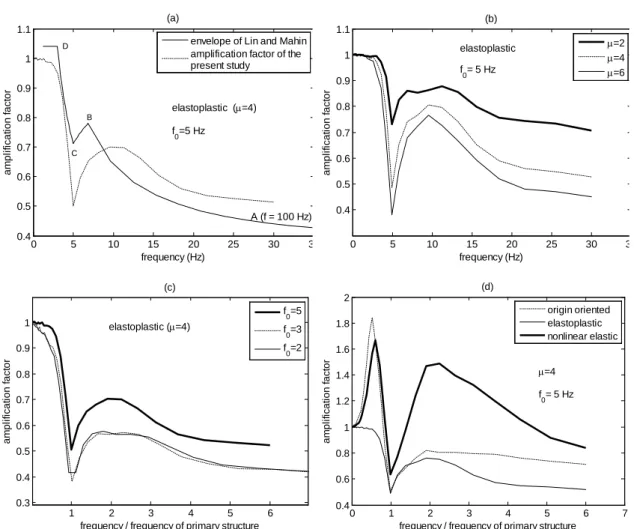
In their study, Lin and Mahin [1], based on the results of nonlinear responses to ten real earthquake records, proposed an envelope of the amplification factor. They define four characteristic points and they propose a linear interpolation between, with respect to the period of the secondary structure. Of course, if plotted versus frequency, this envelope of the amplification factor does not vary linearly. The four characteristic points A, B, C, D correspond respectively to the zero period amplification, to a local maximum, to the minimum and to the beginning of the plateau of low frequency amplification. Figure 3a shows an example of the envelope proposed in [1] as well as the amplification factor issued from the nonlinear response to the excitation signals used in the present study. As it can be seen the envelope of Lin and Mahin does not give a conservative upper bound of the amplification factor in the whole range of frequencies.

Observation of the amplification factor for various structural frequencies, ductility demands and nonlinear constitutive laws leads to the conclusion that the relative location (frequency ratio) of the characteristic points is almost independent of the nonlinear demand, the frequency of the primary structure and the particular nonlinear law. This conclusion is illustrated by the results in figures 3b-3d.

4. EQUIVALENT LINEAR 1DOF OSCILLATOR

Equivalent linear systems are often used by engineers as an approximation of nonlinear systems. In this section we present the properties (frequency and damping ratio) of the equivalent linear 1DOF oscillators leading to floor spectra that are (in some sense) good approximations of the floor spectra of the nonlinear systems. The determination of the equivalent linear oscillator is made a posteriori by a nonlinear least square fitting of the PSD of the acceleration of the nonlinear system.

The square of the modulus of the transfer function of the absolute acceleration of a linear oscillator is:

2 2 2 2 2 2 2 2

)

/

(

4

)

/

1

(

)

/

(

4

1

eq eq eq eq eq a

f

f

f

f

f

f

H

ζ

ζ

+

−

+

=

(1)

The theoretical PSD of a Kanai-Tajimi filtered white noise having a unity PSD has the same expression with feq and

ζ

eq replaced by the frequency and the damping of the filter fg and

g

ζ

respectively. 2 2 2 2 2 2 2

)

/

(

4

)

/

1

(

)

/

(

4

1

g g g g g ee

f

f

f

f

f

f

S

ζ

ζ

+

−

+

=

(2)

So the PSD of the acceleration of the equivalent linear oscillator is

r

S

H

S

_aaeq

=

_a 2 _ee (3)

The coefficient r accounts for the effects of the scaling and of the time modulation envelope applied to the excitation signals used in the nonlinear analyses. If

S

_eenl, is the PSD of the excitation signals, computed numerically,

∫

∫

∞ ∞

=

0 0

df

S

df

S

r

ee nl ee (4)

The parameters feq and

ζ

eq are calculated by least square fitting between eq aa

S

and the PSD

of the acceleration of the nonlinear system. Figure 4 shows the results of the regression analysis for the three types of nonlinear behaviour in the case of a mean inelastic demand

4 =

The results in figures 4b and 4c clearly show that the approximation of an equivalent linear oscillator does not give satisfactory results for the cases of nonlinear elastic and origin oriented models. On the other hand, in the case of an elastoplastic response the fitting shown in figure 4a is quite satisfactory. So, the case of the elastoplastic behaviour will be discussed in more details. Moreover, in order to have a further insight into the behaviour of a nonlinear elastic oscillator an alternative linearization leading to more satisfactory results will also be presented subsequently.

4.1 Equivalent stiffness and damping of an elastoplastic oscillator

A common assumption in earthquake engineering design and reasoning (e.g. [7]) is to approximate the nonlinear behaviour by the behaviour of an equivalent linear oscillator. According to one of the more commonly used methods [7], the frequency is computed by the secant stiffness corresponding to the displacement inelastic demand whereas the damping ratio is the sum of viscous damping and damping corresponding to the energy dissipated by the nonlinear law during a cycle at maximum displacement amplitude.

µ

/

0

f

f

_eq

=

(5)

and for an elastoplastic oscillator :

µ

ζ

µ

π

ζ

_eq = 2(1−1/ )+ ₀ (6)

For the case studied here (initial frequency

f

₀=5 Hz, viscous damping

ζ

₀= 5%, ductility

demand

µ

=4) this approach gives: feq=2.5 Hz and ζeq=58%. In [2] a somewhat different

expression is proposed for the frequency shift and the equivalent damping is estimated without considering the term accounting for plastic dissipation. An extensive presentation of the equivalent linear models proposed so far in the literature can be found in [9].

However the results in figure 4a show that there is no frequency shift and damping is much smaller than the one predicted by eq. (6). In order to better understand the physics of the problem the PSD of the building relative displacement is shown in figure 5.We can see that the energy of the signal is concentrated in the vicinity of zero and 5 Hz frequencies. The general trends of this example are valid for low and moderate ductility demands of practical interest. In fact, the process of the elastoplastic response can be split into two parts. The first one corresponds to the time evolution of the elastic strain (or displacement) and it will be called “elastic” process. The second part, called “plastic”, corresponds to the plastic excursions and it is the remaining part of the signal (total displacement – elastic displacement).The elastic process has a main frequency almost equal to the initial frequency. This is readily explained by the fact that as long as evolution of the plastic deformation does not occur, the behaviour is linear with the stiffness being the initial stiffness during loading and unloading. Moreover, if the ductility demand is not high, the duration of plastic excursions is small, so, the

characteristic time of the process is approximately the period of the associated linear oscillator and its frequency is approximately equal to the initial frequency f0. As far as it concerns the

that in the case of a white noise excitation and if some hardening exists (even small) so that the process may be assumed to be stationary, the PSD of the plastic process is a Dryden spectrum: 2 2 2 2 2 ) f ( ) f ( S_ddp _p

π

λ

λ

σ

+ = (7)

In the above expression

σ

p is the standard deviation and

λ

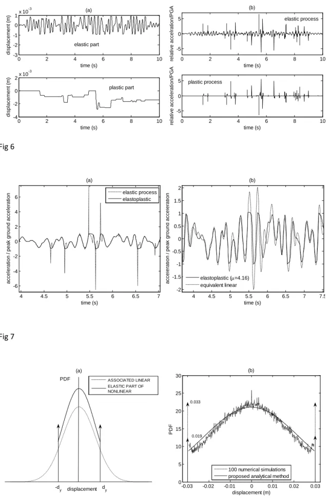
is a frequency dimension

parameter characterizing the mean frequency of the plastic process. This explains the shape of the PSD of fig 5 in the range of low frequencies and the peak at zero frequency. In the case of zero hardening, the shape of the PSD in the vicinity of zero frequency is the same, but, since the plastic part process is no more stationary the intensity of its PSD is time dependent. In figure 6 the relative displacements and accelerations of the elastic and plastic processes of a sample function are shown.

At the beginning of each plastic excursion the velocity of plastic and elastic processes are discontinuous so the corresponding accelerations are Dirac functions. However, because of the continuity of the velocity of the total response, the acceleration Dirac functions of the elastic process have the same absolute value but opposite sign of those of the plastic process, hence their contributions to the total acceleration are mutually cancelled. As it can been seen in figure 7a the absolute acceleration corresponding to the elastic part only is a very good approximation of the acceleration of the elastoplastic response if the Dirac functions are removed.

The extremely good agreement between the PSD of the elastoplastic and equivalent elastic acceleration processes (fig. 4a) implies that the standard deviations of both processes are almost equal. As far as it concerns the displacement process, the standard deviations of the equivalent linear and elastic part processes are found to be almost the same. However, the peak factor of the elastic part process is found to be smaller than the peak factor of the equivalent linear process. Indeed, the probability density function of the elastic part is quite different from the one of the equivalent linear process because the displacement cannot take values in the entire domain

]

− ,

∞

+

∞

[

. As it can be seen in figure 7b the maximum

acceleration of the linear equivalent response is higher than the one of the elastoplastic response. For this reason, the value of the plateau of the floor spectrum at high frequencies is higher for the linear equivalent oscillator than for the elastoplastic oscillator.

The equivalent damping ratios for different ductility demands and frequencies are presented in table 1. For the sake of comparison in the same table the equivalent damping given by eq. (6) divided by

µ

so as to correspond to the damping ratio with respect to the initial frequency is listed also. It is worth noticing that in contrast to equation (6) the damping ratio corresponding to plastic dissipation increases almost linearly with increasing ductility demand and it depends on the frequency of the structure.

In the following we propose a method to approximate a priori the damping of the equivalent linear oscillator in the case of a white noise excitation (or a wide band excitation). At first we consider the response of a linear elastic oscillator with the initial damping (e.g. 5% for the examples considered). This process will be called associated linear process. Its probability density function (PDF) is a normal distribution with zero mean value and variance given by the classical relation: 0 3 0 0 2

2

ω

ζ

ω

π

σ

S

ee

(

)

d

=

(8)

where See is the two sided PSD of the excitation. The PDF of the elastic part of the elastoplastic

solution is different. In particular it is defined in the [−d_y,d_y] domain with two Dirac functions at the boundaries accounting for the displacement values on the plateau of the elastic part of the solution (figure 8a). We make the assumption that the PDF of the elastic part (excepted the Dirac functions) is equal to the truncated PDF (between −d_y and d_y) of the associated linear process scaled by an amplification factor. By definition, the area under this function must be equal to one. In the case of low ductility demands we can, in a first

approximation, neglect the contribution of the Dirac functions to the computation of the probability function (a reasonable approximation when plastic excursions are of limited

duration and/or are not very frequent). The condition of unit area under the PDF curve enables the computation of the scaling factor and thus of the PDF of the elastic part of the nonlinear response. The numerical computation of the standard deviation is straightforward and the equivalent damping

ζ

eq can be estimated by eq. (8), if

ζ

eq is used in place of

ζ

0.

As an example we examine an elastic perfectly plastic oscillator having a 5 Hz frequency and a 5% damping. A small hardening would have given similar results, but the choice of no

hardening has been made for the sake of consistency with the theory presented in this

subsection. The yield force is determined to result in an average ductility demand of two under a white noise excitation having a duration of 20 s. The above procedure gives a damping of 7% which is in good agreement with the value of 6.5 %, given by the least square fitting of the PSD. However, neglecting the contributions of the Dirac functions results in a lower standard deviation and consequently to higher damping values. Obviously, the differences between the results of the above simplified procedure and the consistent linearization by fitting of the PSD are even more important in the case of higher (moderate) ductility demands. So, the need to take into account the Dirac functions contributions arises. To this purpose we use the results of the pioneering work of Vanmarcke and Veneziano [11]. According to their results the mean time between plastic excursions of an elastic perfectly plastic oscillator submitted to a white noise excitation is:

(

q

)

p e f e t _{π η} η 2 / 0 2 / 2 1 2 − − = (9)

where

η

=d_y /

σ

_d is the normalized yielding displacement and q is a measure of the spread of the band of the associated linear process:

π

ζ

λ

λ

λ

ζ 0 1 0 2 0 2 1 4 1 0 . if q < ≅ − = (10) 0

λ

,

λ

1 and

λ

2 being the moments of the spectral density of the process of order 0, 1 and 2 respectively. Attention must be given to the fact that plastic excursions occur in clumps and the above mean time t_p is an approximation of the mean time between successive plastic clumps.

It can be proven that the average velocity of crossing a given level for a linear elastic process does not depend on the level itself and its value is:

v

=

2

π

f

₀

σ

_d

π

/

2

(11)

In the following we will consider that instead of clumps there is only one plastic excursion at a time. This assumption is motivated by our wish for simplification and does not correspond to a physical reality. However, it is consistent with the observation that in the case of low ductility demand (high yield force) the number of plastic jumps in a clump is small, one plastic jump being a limit case. If we make also the assumption that the velocity of crossing (reaching) the yield level is the same as for the associated linear process, the average duration of a plastic excursion may be computed by considering that the yielding force decelerates the mass m of the oscillator up to a zero velocity before an unloading elastic phase begins:

∆

t_p =vm/F_y. It results that the probability that the displacement takes the yield value d_y or −d_y is:

p p y

t

t

d

d

P

(

=

)

=

∆

/

(12)

Consequently the amplitude of the Dirac functions of the PDF is0.5

∆

t /_p t_p. The PDF based on the above assumptions is compared in figure 8b with the PDF computed by means of 100 numerical simulations. It must be recognized that the proposed method, based, as already mentioned, on the assumption of one plastic jump at a time instead of a clump of plastic jumps in alternating directions, underestimates the amplitude of the Dirac functions because the duration of the plastic excursions is underestimated. Consequently, the variance is

underestimated and hence the equivalent damping is slightly overestimated. For example, for the case shown in figure 8b ( f₀ =5 Hz,

ζ

₀ =0.05,

π

S

_ee

/

2

ω

₀3

ζ

₀

d

2_y

=

0

.

57

) we find a

damping of 9.8% instead of 9.32% as determined by the PSD fitting. Despite this small discrepancy the agreement is considered satisfactory. On the basis of various numerical simulations, not shown here for lack of available space, it seems that a conservative estimate of the damping would be to multiply the analytical determined Dirac functions by 1.6. For the case discussed here this leads to a damping of 9.1%.

In the case of a filtered white noise excitation, like the Kani-Tajimi filtered white noise considered here, the equivalent damping can be approximated if we make the usual

assumption that a white noise excitation can be considered, having a PSD value equal to the PSD value of the filtered excitation process at the frequency of the oscillator. In figure 4a we can see that, for the example case previously examined, the fitting of the PSD gives an

equivalent damping of 12.2 %. The simplified variant (neglecting the contributions of the Dirac functions) of the method proposed in this section gives an equivalent damping of 11.25 %. Although the agreement is satisfactory, it must be recognized that contrary to the case of a white noise excitation where the analytical method (especially the simplified variant) overestimates the damping, in this case the damping is underestimated. This discrepancy is due to the fact that because of the filtering process, as well as of the temporary scaling of the excitation signals, eq. (8) is less accurate than in the case of a pure white noise. This is true even if the response is completely linear. For instance, the use of eq. (8) to determine the damping of the elastic process, knowing the standard deviation, gives a 4.5 % damping instead of the exact value of 5 %.

4.3. An alternative concept of equivalent linearization of a nonlinear elastic oscillator As already mentioned in section 4, replacing a nonlinear elastic oscillator with an equivalent linear oscillator, having a constant stiffness, does not give satisfactory results, at least as far as the frequency content of the response is concerned. This is clearly illustrated in figure 4c. In this section we will present an alternative method of linearization, based on an equivalent linear oscillator whose frequency is a random variable. The method deals with oscillators with nonlinear stiffness force that can be derived from a potential. It has been presented firstly in the pioneering work of Guihot [12] and Miles [13] and has been improved later by Bouc [14], Bellizzi and Bouc [15], Fogli et al [16] and Rudinger and Krenk [17]. All the examples treated in these references concern systems with tangential stiffness increasing with deformation (e.g. Duffing oscillator or impacting oscillator). However, there is no limitation in the theory to account for tangential stiffness decreasing with deformation, as it is the case in this study, provided that there is not softening behaviour (no negative tangential stiffness). Even if the practical interest of the method is perhaps limited, it has a theoretical interest and contributes to having a further insight into the physics of the problem. For the sake of simplicity, we will limit ourselves to the case of a white noise excitation, although the theory can be applied to general wide band random excitations. One of the basic ideas is that the main apparent circular frequency of the response Ω depends on the value of the envelope of the process b (

) (b

b→

Ω

). We remind that the envelope amplitude b corresponding to a displacement d

and a velocity

d

can be defined implicitly by:

) ( ) ( ) (b U d K d U = +  (13)

where U and K are the potential and kinetic energy respectively and

b

≥

0

. The apparent

frequency

Ω

(b), corresponding to a cycle with maximum amplitude b, is calculated by considering the conservative free oscillations of the same amplitude. Energy conservation leads to:

















>

































−

−

+

≤

=

y y y y y

d

b

if

b

d

b

d

b

d

b

d

b

if

b

2 2 2 0 2 0 2

1

cos

2

1

)

(

π

α

ω

ω

Ω

(14)

where dy is the displacement corresponding to the limit of linear behaviour and

(

k

2

−

k

1

)

/ k

1

=

α

, 2 0 1

=

ω

k

and

k

₂ being the linear and post-linear stiffness. The next step is

to approximate the nonlinear stiffness force with

Ω

2(b)d. The resulting equation of motion reads: g

d

d

b

d

d





+

2

ζ

₀

ω

₀



+

Ω

2

(

)

=

−





(15)

where

d

is the relative displacement and

d



_g is the ground acceleration. Attention must be

paid to the fact that, in accordance with the physics, the damping force is not amplitude dependent.

Numerical solutions of eq. (15) (with b(t) having been calculated previously from the original nonlinear equation) show that the mean error of the force estimate is small, although locally (at each time instant) it may be significant. Moreover, as it can be observed in figure 9a, the displacement corresponding to the equivalent linear system with varying stiffness coefficient of eq. (15) is an excellent approximation of the nonlinear response.

Under the assumption of a narrow band process, the probability density function of the envelope is given by [18]:

)

(

/

)

(

)

(

b

C

p

z

b

p

=

_b

Ω

(16)

where p(z) is the PDF of the peaks given by:













−

=

0 0 0

(

)

2

exp

)

(

)

(

S

z

U

dz

z

dU

C

z

p

_z

π

ω

ζ

(17) In the above expressions

C

b and

C

z are normalisation constants, U(z)is the potential energy and

S

0 is the two sided PSD of the white noise excitation.

Miles [19] deals with equation (15). In order to calculate the PSD of the displacement response he proceeds in a manner analogous to the one classically used in the case of constant stiffness coefficient making the assumption that, for a known time history of b(t), the Green function (impulsive response) may be approximated by the expression:

) ( sin 1 ) ( ( )/2

ω

τ

ω

τ

₌ τ ₋ − − − t e t h c t _D D (18) where 2 0 2 0 2

))

(

(

ζ

ω

Ω

ω

_D

=

b

t

−

. It is worth noticing that

ω

_D is a function of the time t and

not of t−

τ

. The above approximation is based on the assumption that

Ω

2(b)varies much more slowly than h(t−

τ

). It follows that the displacement history is given by the convolution integral:

∫

− = t g d d t h t d 0 ) ( ) ( ) (

τ



τ

τ

(19)

The resulting PSD of the displacement is:

(

)

p b db b S S_dd ( ) 4 ) ( 1 ) ( 0 2 2 0 2 0 2 2 2 0

∫

∞ + − =

ω

ω

ζ

ω

Ω

ω

(20)

However the approximation of the Green function of the linear equation with varying stiffness coefficient by relation (18) is not accurate. In fact, figure 9b shows the solutions of eq. (15) computed by a time integration algorithm and by the convolution integral (19) using the approximation (18) for the impulsive function. It becomes obvious that this approximation is not satisfactory and that, therefore, the PSD given by eq. (20) is not accurate in the case of strong nonlinearities.

Instead of considering eq. (15) one can consider the following equation: g

d

b

B

d

b

d

d





+

2

ζ

₀

ω

₀



+

Ω

2

(

)

=

−

(

)





(21)

where

b

is a random variable independent of the white noise input

d



_g. For a given value of

the random variable b, B(b) is calculated by seeking the mean square displacement of the linear eq. (21) to be equal to the mean square value of the nonlinear response, which reads

2

/

)

2

/

(

)

(

d

2

E

b

2

b

2

E

_nl

=

=

[14]. So:

2

)

(

2

)

(

2 2 0 0 0 2 2

b

b

S

B

d

E

=

=

Ω

ω

ζ

π

(22)

It results that the intensity of the white noise

S

₀ is replaced by

B

2

S

₀

=

b

2

ζ

₀

ω

₀

Ω

2

(

b

)

/

π

.

For fixed b, the conditional PSD of the displacement is:

(

)

2 2 0 2 0 2 2 2 2 0

4

)

(

)

(

)

/

(

ω

ω

ζ

ω

Ω

ω

+

−

=

b

b

B

S

b

S

_dd (23)

It follows that the PSD is given by:

(

)

p b db b b B S S_dd ( ) 4 ) ( ) ( ) ( 0 2 2 0 2 0 2 2 2 2 0

∫

∞ + − =

ω

ω

ζ

ω

Ω

ω

(24)

The PSD of other response variables of interest are calculated with the same procedure. For example the PSD of the absolute acceleration is:

(

)

(

)

p

(

b

)

db

)

b

(

)

b

(

B

)

b

(

S

)

(

S

_aa

∫

∞

+

−

+

=

0 2 2 0 2 0 2 2 2 2 4 2 2 0 2 0 0

4

4

ω

ω

ζ

ω

Ω

Ω

ω

ω

ζ

ω

(25)

Figure 10 compare the PSDs calculated according to the preceding method with the results of numerical simulations (

S

₀

=

0

.

5

m2/s3r,

f

₀

=

5

Hz, d_y =0.0264m,

α

=

−

0

.

99

,

ζ

₀

=

0

.

05

).

Despite some discrepancies the agreement is good. The proposed method captures the broadening of the PSD and clearly explains that this is not the consequence of increasing damping but of frequency scattering. However, it must be noticed that numerical simulations show that the time history of the displacement of the modified equivalent linear equation (21) is a poorer approximation of the exact displacement of the nonlinear system than the solution of eq. (15) (both

Ω

(b) and B(b)having being previously determined by the solution of the original nonlinear equation).

It can be mathematically proven [14] that if the nonlinear stiffness force is expressed in terms of Fourier series, the above method corresponds to the first order approximation with only one term retained. A refinement of the method, taking into account higher order terms reveals the appearance of odd harmonics ((2n−1)

Ω

(b)) especially in the PSD of the acceleration. These higher harmonics may explain the local maximum of the

pseudoacceleration spectra in figure 2. Actually, in section 3 we observed a small local peak at a frequency about 2 times the initial frequency. However, considering the reduction of the apparent frequency and the shape of the PSD of the excitation input (which is not a white noise), one can speculate that these local maxima may correspond to the third harmonic

) (

3

Ω

b .

5. DESIGN FLOOR SPECTRA OF PRIMARY STRUCTURES WITH ENERGY DISSIPATING CAPACITY

This section concerns only primary structures having an elastoplastic or origin oriented behaviour, that is, the two types of behaviour of this study with some energy dissipation capacity. The term equivalent linear oscillator is used in this section to designate the linear oscillator equivalent to the elastoplastic oscillator.

As already mentioned in section 3, the peak floor spectral values given by the origin oriented model and located in the vicinity of the initial frequency f0, are lower or similar to the peak

values corresponding to the elastoplastic behaviour. Observation of the results of section 3 shows, also, that for frequencies higher than f0 the floor spectra for both types of behaviour

are similar. This means that, for this range of frequencies, the floor spectrum of the elastoplastic case may be used as an approximation of both spectra. In addition, as already mentioned in subsection 4.1 the maximum acceleration (and consequently the floor spectral acceleration plateau at high frequencies) is higher in the case of the equivalent linear oscillator than in the case of the elastoplastic oscillator. So, we can consider that the floor spectrum of the equivalent linear oscillator lies over or near the floor spectra corresponding to these two types of nonlinear behaviour for frequencies higher than f0. Observation of the results of

oriented behaviour are higher than those of the elastoplastic structure. We speculate that a plateau from f0 to f0/2 and a linear interpolation up to zero frequency would add sufficient

margin to the floor spectrum in the range of frequencies between zero and f0. So, we can

summarise a proposal for a design floor spectrum of structures exhibiting some energy dissipation, in the following steps:

- determine the equivalent linear oscillator for an elastoplastic behaviour for a given nonlinear demand,

- use the floor spectrum of this equivalent linear oscillator in the frequency range from the primary structure frequency,

f

0, to infinite frequency,

- consider a horizontal plateau from

f

₀ to

f

₀

/

2

,

- linearly interpolate between zero frequency and

f

₀

/

2

.

As illustrated in figure 11, the resulting design spectrum, lies over or near the floor spectrum values corresponding to the elastoplastic and origin oriented models

6. CONCLUSIONS

In this work we tried to have a better understanding of the influence of nonlinear earthquake response of 1DOF primary structures to the floor spectra. In accordance to the findings of previous studies [1], the observation of the results of numerical simulations confirms that: - In general, nonlinear behaviour of the primary structure reduces the peak values of the

floor spectra.

- However, nonlinear behaviour does not, always, result in floor spectral values which lie under the floor spectral values of the corresponding linear structure in the whole range of frequencies.

Moreover, the main conclusions of this study can be summarised as follows:

- Generally, for the same inelastic demand, and for skeleton curves of the same shape, energy dissipating nonlinear behaviour seems to result in lower spectral values than nonlinear behaviour without energy dissipation.

- The effect of an elastoplastic behaviour of the primary structure on the floor spectrum can be satisfactorily reproduced by the consideration of an equivalent linear oscillator.

Contrary to some common approaches, the stiffness of the equivalent linear oscillator is the stiffness of the initial linear oscillator and the damping is much less than the damping given by the hysterisis area at maximum displacement cycle.

- A method is proposed to determine a priori the damping of the equivalent linear oscillator in the case of elastoplastic behaviour and a large band excitation defined by its power spectral density.

- The method of equivalent linearization with the equivalent frequency being a random variable is applied, in the case of an elastic nonlinear oscillator, and gives power spectral densities in a satisfactory agreement with the results of numerical simulations.

- A proposal of a design floor spectrum of primary structures exhibiting energy dissipating nonlinear behaviour is presented.

The most important limitations of this paper concern the assumption of 1DOF primary structures and the models of idealized nonlinear behaviour considered. Studies with a larger variety of nonlinear laws should be performed to enhance (or weaken) the validity of the above conclusions and observations. The issue of floor spectra of nonlinear multi-degree of freedom primary structures is much more complex. The authors are working in this field and they hope to publish their results in the near future.

ACKNOWLEDGEMENTS

This work is partially financed by the integrated project LESSLOSS of the European Union. This financial support is gratefully acknowledged by the authors.

REFERENCES

1. Lin J, Mahin S. Seismic Response of Light Subsystems on Inelastic Structures. Journal of

Structural Engineering 1985; 111(2):400-417.

2. Villaverde R. Simplified Approach to Account for Nonlinear Effects in seismic Analysis of Nonstructural Components. Seminar on seismic design, retrofit and performance of

non-structural components 1998; ATC-29-1:187-200.

3. Sewell RT, Cornell CA, Toro GR, McGuire RK, Kassawara RP, Sing A. Factors influencing equipment response in linear and nonlinear structures. Transactions of 9th _{international} conference on Structural Mechanics In Reactor Technology, Lausanne, Switzerland, 1989; K2:849-856.

4. Singh MP, Chang TS, Suarez LE. Floor response spectrum amplification due to yielding of supporting structure. Proceedings of 11th _{World Conference on Earthquake Engineering,}

Acapulco, Mexico, 1996; Paper No. 1444.

5. Villaverde R. Method to improve seismic provisions for non-structural components in buildings. Journal of Structural Engineering 1997; 123(4):432-439.

6. Rodriguez ME, Restrepo JI, Carr AJ. Earthquake-induced floor horizontal acceleration in buildings. Earthquake Engineering and Structural Dynamics 2002; 31:693-718.

7. Priestley MJN. Myths and Fallacies in Earthquake Engineering Revisited; The Mallet Milne Lecture, IUSS Press, 2003.

8. Pinto PE, Vanzi I. Base Isolation: Reliability for different design criteria. Proceedings of 10th World Conference on Earthquake Engineering, Rotterdam, Balkema, 1992; 2033-2038.

9. Miranda E, Ruiz-Garcia Jorge. Evaluation of approximate methods to estimate maximum inelastic displacement demands. Journal of Earthquake Engineering and Structural

Dynamics 2003; 32(8):1237-1258.

10. Feau C. Les méthodes probabilistes en mécanique sismique. Application aux tuyauteries

fissurées. Thèse de Doctorat de l’Université d’Evry, 2003.

11. Vanmarcke EH, Veneziano D. Probabilistic seismic response of simple inelastic systems. 5th World Conference on Earthquake Engineering 1973; Rome.

12. Guihot P. Analyse de la réponse de structures non-linéaires sollicitées par des sources

d’excitation aléatoires. Application au comportement des lignes de tuyauteries sous l’effet d’un séisme. Thèse de Doctorat de l’Université Paris VI, 1990.

13. Miles RN. An approximate solution for the spectral response of Duffing’s oscillator with random input. Journal of Sound and Vibration 1989; 132(1):43-49.

14. Bouc R. The power spectral density of response for a strongly non-linear random oscillator.

Journal of Sound and Vibration 1994; 175(3):317-331.

15. Bellizzi S, Bouc R. Spectral response of asymmetrical random oscillators. Probabilistic

Engineering Mechanics 1996; 11:51-59.

16. Fogli M, Bressolette Ph, Bernard P. The dynamics of a stochastic oscillator with impacts.

European Journal of Mechanics and Solids 1996; 15(2):213-241.

17. Rundinger F, Krenk S. Spectral density of oscillator with bilinear stiffness and white noise excitation. Probabilistic Engineering Mechanics 2003; 11:51-59.

18. Lin YK. Probabilistic Theory of Structural Dynamics; McGraw-Hill, 1967.

19. Miles RN. Spectral response of a bilinear oscillator. Journal of Sound and Vibration 1993;

163(2):319-326.

20.

Table 1: Equivalent damping ratios (in %) for various structural frequencies and ductility demands

frequency ductility

2 Hz 3 Hz 5 Hz

PSD _Eq(6)/ PSD _Eq(6)/ µ PSD Eq(6)/

µ

1 5 5 5 5 5 5

2.5 12 29.1 10.6 29.1 8.6 29.1

4 19 28.8 16.6 28.8 12.2 28.8

Figure captions

Fig. 1: Nonlinear constitutive laws.

Fig. 2: Floor spectra (mean of 100 signals) of a building exhibiting a mean nonlinear displacement demand µ=4 and having a frequency of: (a) 2 Hz; (b) 3 Hz; and (c) 4 Hz. Fig. 3: Amplification factor: (a) comparison with the envelope of Lin and Mahin; (b) various ductility demands; (c) various frequencies; and (d) various nonlinear constitutive laws. Fig. 4: Least square fitting of the power spectral density of the floor acceleration of a primary structure having an initial frequency of 5 Hz: (a) elastoplastic; (b) origin oriented; and (c) nonlinear elastic.

Fig. 5: Power spectral density of the displacement of the primary structure (f0 = 5 Hz, μ= 4).

Fig. 6: Partitioning of relative displacement and accelerations to elastic and plastic parts (µ=4.16).

Fig. 7: Acceleration time history of a time segment of a sample function (µ=4.16): (a) elastic part and elastoplastic processes; and (b) elastoplastic and equivalent linear processes. Fig. 8: Probability density function of the elastic part of the elastoplastic response process. Fig. 9: Displacement time history of the elastic nonlinear oscillator for a time segment of a sample function: (a) comparison between the original nonlinear oscillator and the equivalent linear oscillator of eq. (15); and (b) comparison between solutions of the equivalent linear oscillator, computed by central differences and by the convolution integral with the impulsive response approximated by eq. (18).

Fig. 11: Comparison between the proposed design floor spectrum and numerically determined floor spectra (means of 100 signals) for a primary structure with a mean ductility demand μ = 4 and having a frequency of: a) 5 Hz ; and (b) 3Hz.

FIGURES

a) elastoplastic b) origin oriented c) nonlinear elastic

Fig.1 d F d F d F 0 5 10 15 20 25 30 35 0 5 10 15 frequency (Hz) ps eudoac c el er at ion / peak gr ound ac c el er at ion (a) linear elastoplastic origin oriented nonlinear elastic f₀=2 Hz 0 5 10 15 20 25 30 35 0 5 10 15 20 25 frequency (Hz) ps eudoac c el er at ion / peak gr ound ac c el er at ion (b) linear elastoplastic origin oriented nonlinear elastic f 0=3 Hz 0 5 10 15 20 25 30 35 0 5 10 15 20 25 frequency (Hz) ps eudoac c el rat ion / peak gr ound ac c el er at ion (c) linear elastoplastic origin oriented nonlinear elastic f 0=5 Hz

Fig. 2 Fig. 3 0 5 10 15 20 25 30 3 0.4 0.5 0.6 0.7 0.8 0.9 1 1.1 frequency (Hz) am pl if ic at ion f ac tor (a)

envelope of Lin and Mahin amplification factor of the present study C B A (f = 100 Hz) D elastoplastic (µ=4) f 0=5 Hz 0 5 10 15 20 25 30 3 0.4 0.5 0.6 0.7 0.8 0.9 1 1.1 (b) frequency (Hz) am pl if ic at ion f ac tor µ=2 µ=4 µ=6 elastoplastic f₀= 5 Hz 1 2 3 4 5 6 0.3 0.4 0.5 0.6 0.7 0.8 0.9 1

frequency / frequency of primary structure

am pl if ic at ion f ac tor (c) f 0=5 f 0=3 f₀=2 elastoplastic (µ=4) 0 1 2 3 4 5 6 7 0.4 0.6 0.8 1 1.2 1.4 1.6 1.8 2 am pl if ic at ion f ac tor

frequency / frequency of primary structure (d) origin oriented elastoplastic nonlinear elastic µ=4 f 0= 5 Hz

Fig 4 Fig. 5 0 5 10 15 20 25 30 0 2 4 6 8 10 12 14 frequency (Hz) P S D of f loor ac c el er at ion (a) elastoplastic equivalent linear f eq=4.93 Hz, ζeq=12.2% 0 5 10 15 20 25 30 0 2 4 6 8 10 12 14 16 18 20 frequency (Hz) P S D of f loor ac c el er at ion (b) origin oriented equivalent linear f eq=3.14 Hz, ζeq=15.8% 0 5 10 15 20 25 30 0 5 10 15 20 25 30 frequency (Hz) P S D of f loor ac c el er at ion (c) nonlinear elastic equivalent linear f eq=4.7 Hz, ζeq=8.7% 0 5 10 15 20 25 30 10-10 10-8 10-6 10-4 10-2 frequency (Hz) P S D of r el at iv e di s p lac em ent f₀ = 5 Hz ζ 0 = 5% µ = 4

Fig 6 Fig 7 0 2 4 6 8 10 -3 -2 -1 0 1x 10 -3 time (s) di s pl ac em ent ( m ) (a) 0 2 4 6 8 10 -4 -2 0 2x 10 -3 time (s) di s pl ac em ent ( m ) plastic part elastic part 0 2 4 6 8 10 -5 0 5 time (s) rel at iv e ac c el rat ion/ P G A (b) 0 2 4 6 8 10 -5 0 5 time (s) rel at iv e ac c el er at ion/ P G A plastic process elastic process 4 4.5 5 5.5 6 6.5 7 -6 -4 -2 0 2 4 6 time (s) ac c el er at ion / peak gr ound ac c el er at ion (a) elastic process elastoplastic 4 4.5 5 5.5 6 6.5 7 7.5 -2 -1.5 -1 -0.5 0 0.5 1 1.5 2 time (s) ac c el er at ion / peak gr ound ac c el er at ion (b) elastoplastic (µ=4.16) equivalent linear (a) ASSOCIATED LINEAR ELASTIC PART OF NONLINEAR PDF displacement -d y dy -0.03 -0.02 -0.01 0 0.01 0.02 0.03 0 5 10 15 20 25 30 displacement (m) P D F (b) 100 numerical simulations proposed analytical method

0.033

Fig 8 Fig 9 Fig 10 11 11.5 12 12.5 13 -0.1 -0.05 0 0.05 0.1 time (s) di s pl ac em ent ( m ) (a) equivalent linear non linear 7.5 8 8.5 9 9.5 1 -0.1 -0.08 -0.06 -0.04 -0.02 0 0.02 0.04 0.06 0.08 time (s) di s pl ac em ent ( m ) (b) central differences convolution integral 0 2 4 6 8 10 0 1 2 3 4 5 6x 10 -5 Sd d (ω ) ( m 2s /r ) frequency (Hz) (a) nonlinear equivalent linear 0 2 4 6 8 10 0 5 10 15 20 25 30 frequency (Hz) Saa (ω ) ( m 2/s 3r) (b) nonlinear equivalent linear

Fig 11 0 1 2 3 4 5 6 7 0 2 4 6 8 10 12 f/f 0 ps eudoac c el er at ion/ peak gr ound ac c el er at ion (a) proposal elastoplastic origin oriented

floor spectrum of the equivalentlinear oscillator of the elastoplastic case

f 0=5Hz, µ=4 0 2 4 6 8 10 12 0 2 4 6 8 10 12 f/f 0 ps eudoac c el er at ion/ peak gr ound ac c el er at ion (b) proposal elastoplastic origin oriented f 0=3 Hz, µ=4

floor spectrum of the equivalent linear oscillator of the elastoplastic case