HAL Id: cea-02500852
https://hal-cea.archives-ouvertes.fr/cea-02500852
Submitted on 6 Mar 2020
HAL is a multi-disciplinary open access
archive for the deposit and dissemination of
sci-entific research documents, whether they are
pub-lished or not. The documents may come from
teaching and research institutions in France or
abroad, or from public or private research centers.
L’archive ouverte pluridisciplinaire HAL, est
destinée au dépôt et à la diffusion de documents
scientifiques de niveau recherche, publiés ou non,
émanant des établissements d’enseignement et de
recherche français ou étrangers, des laboratoires
publics ou privés.
R.I.A. experiments Acoustic Emission signal analysis
L. Pantera, O. Issiaka Traore
To cite this version:
L. Pantera, O. Issiaka Traore. Reproducible Data Processing Research for the CABRI R.I.A.
experi-ments Acoustic Emission signal analysis. ANIMMA 2015 - 4th International Conference on
Advance-ments in Nuclear Instrumentation Measurement Methods and their Applications, Apr 2015, Lisbonne,
Portugal. �cea-02500852�
Reproducible Data Processing Research for the
CABRI R.I.A. experiments Acoustic Emission signal
analysis
Laurent Pantera
∗,Oumar Issiaka Traore
†∗
CEA, DEN, CAD/DER/SRES/LPRE, Cadarache, F-13108 Saint-Paul-lez-Durance, France
†Laboratory of Machanics and Acoustics (LMA) CNRS, 13402 Marseille FRANCE
Abstract—The CABRI facility is an experimental
nu-clear reactor of the French Atomic Energy Commission (CEA) designed to study the behaviour of fuel rods at high burnup under Reactivity Intitiated Accident (R.I.A.) conditions such as the scenario of a control rod ejection. During the experimental phase, the behaviour of the fuel element generates acoustic waves which can be detected by two microphones placed upstream and downstream from the test device. Studies carried out on the last fourteen tests showed the interest in carrying out temporal and spectral analyses on these signals by showing the existence of signatures which can be correlated with physical phenomena. We want presently to return to this rich data in order to have a new point of view by applying modern signal processing methods. Such an antecedent works resumption leads to some difficulties. Although all the raw data are accessible in the form of text files, analyses and graphics representations were not clear in reproducing from the former studies since the people who were in charge of the original work have left the laboratory and it is not easy when time passes, even with our own work, to be able to remember the steps of data manipulations and the exact setup. Thus we decided to consolidate the availability of the data and its manipulation in order to provide a robust data processing workflow to the experimentalists before doing any further investi-gations. To tackle this issue of strong links between data, treatments and the generation of documents, we adopted a Reproducible Research paradigm. We shall first present the tools chosen in our laboratory to implement this workflow and, then we shall describe the global perception carried out to continue the study of the Acoustic Emission signals recorded by the two microphones during the last fourteen CABRI R.I.A. tests.
Index Terms—Reproducible Research, R language,
Acoustic Emission, CABRI R.I.A. tests
I. Introduction
T
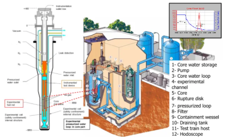
HE CABRI facility is an French experimental nuclear reactor located at the Cadarache Research Centre in southern France. CABRI is made up of an experimental loop specially designed (see figure 1):• to receive the instrumented test device housing the fuel rod to be tested in the centre of the driver core. This device also includes the instrumentation to control the experiment and to characterize the behaviour of the fuel rod during the power transient,
• to cool the experimental fuel rod in the required
thermal-hydraulic conditions.
The LPRE laboratory of the CEA is in charge of the preparation and performance of the tests. Early after a test, its responsibilities also include a preliminary inter-pretation of the experimental data from signals obtained by many sensors placed within the experimental cell.
1- Core water storage 2- Pump 3- Core water loop 4- experimental channel 5- Core 6- Rupture disk 7- pressurized loop 8- Filter 9- Containment wessel 10- Draining tank 11- Test train host 12- Hodoscope
Figure 1: Experimental pressurized water loop (155 bar, 300◦C) with the test device
In this article, We shall focus in the article only on microphone signals placed upstream and downstream from the test device. The main phenomenon to be tracked is the fuel rod failure. It is our ambition to return to the data of the last fourteen tests, carried out from the year 1993 to 2002, in order to highlight specific events which would have been precursors of the rod failure. We therefore had to face a classic problem for experimentalists managing large data sets. People who did the work left the laboratory and in spite of technical notes it is not easy to answer the following questions:
1) Choice of the raw experimental data among all the files acquired for every experiment,
2) Data cleaning (digitizing date correction, up-sampling, not identical sensors names along the years...),
3) Method to detecting abrupt changes in the micro-phone signals to generate events,
4) Parameter settings for treatments on the data and graphic representations of the results,
5) Control of the global coherence of the process. Moreover, the difficulty in applying this process is that, in real life, it never flows smoothly from data collection to conclusions. We must repeat many parts of the break-down discovering problems with the data, find the right adjustment of parameters to recover the old results and then finally apply new data analysis methodologies which may make a better use of the data. In fact, the important principle in our case, and generally in data processing, is iteration. We discovered there was a way to run it using the Literate Programming paradigm. Introduced for writing good software documentation with its maintenance as time passes, it is really worth exploring this orientation to work in data processing. The object of the work presented in this article is to demonstrate how we put this iteration princi-ple in action in our laboratory. We shall first present the principle of the Literate Programming, then the software tools chosen to implement this workflow, and finally we shall describe the global perception carried out to continue the study of the Acoustic Emission signals recorded by the two microphones during the last fourteen CABRI R.I.A. tests.
II. Literate Programming
A. General description
The idea comes from computer science. “Literate Pro-gramming” is a programming methodology devised by Knuth [1]. The aim was to create significantly better documentation of programs and also to provide a realistic means to help the programmers keep the documentation up to date according to the code evolution given the fact that the code and the documentation would be embedded in the same file. In fact, Knuth explains that rather than considering a program to be a set of instructions to a computer that includes comments to the reader, it should be seen as an explanation to a human with a corresponding code. Two processors called “tangle” and “weave” allow us to convert the original source document into an ex-ecutable program and into a publishable document in high quality, respectively (i.e. with a table of contents, references, algorithms, figures etc...), the typesetting being managed by the TEX/LATEX langage [2]. The first Literate
Programming environment called WEB [3] was designed by Knuth. There were then many other tools, often tied to a specific programming language, not always easy to learn. A simplified approach, called "noweb", was then proposed by Ramsey [4]. This solution requires the use of only one file with a minimum syntax to be learned. We shall now describe this way to process.
B. The noweb solution
A noweb file is a text file containing "code delim-iters" called chunks which separate code instructions from the documentation. Each code chunk begins with <<
chunk name >>= on a line by itself and we have to
give it a name. Each documentation chunk begins with a line that starts with an @ on a line by itself also, without name. Chunks are terminated implicitly by the beginning of another chunk or by the end of the file. The documentation chunks contain text written in LATEX.
The Literate Programming tools help the user extract the code from the code chunks in order to compile, execute it and construct the documentation by extracting the LATEX instructions from the documentation chunks. The
supported langages depend on the Literate Programming tool used.
C. The R Language
In our laboratory, we have been working for some years with the free powerfull software R [5] for data manipulation and calculation. This software proposes an implementation of the noweb approach described in the previous section for doing Literate Programming. R has two special functions, Sweave [6] and knit [7] to process the noweb file where the text of a document is "woven" with the code written to perform calculations and produce the figures, the tables presenting the results. The processed file is another text file containing the LATEX instructions
of the documentation chunks and where the code chunks have been replaced by the results of their evaluation.
III. setting up the Laboratory notebook We give the software chosen to work in our laboratory.
A. Editor
At the beginning of our approach, we worked with
Tinn-R [8]. It is a very nice editor, easy to use and very
efficient for using with the R and LATEX languages. More
recently, appeared RStudio [9] which is a powerful IDE1 dedicated to R. With skill, we may prefer to use Emacs [10] with the add-on package ESS (Emacs Speak Statistics). The package is designed to support editing of scripts and interaction with various statistical analysis programs such as R. Although the learning curve is not steep, emacs is a text editor with lots of great features very convenient when one knows how to use them in the everyday life manipulating data.
B. Data Manipulation
As we already stated, we mainly use the R language but we also use the python and octave languages as well as the very convenient unix command, awk which are also supported by the knit function.
C. Data Storage
We decided to manage the detected events with the DBMS2 PostegreSQL. It has the advantage of being very
well interfaced with the R Language.
1Integrated Development Environment
D. Versioning
We track the different versions of some files with the git software [11]. The type of files under versioning can vary a lot, from the quality insurance header of the laboratory technical report, the bibliography or even the mock data for testing code. Git was chosen due to the fact that it is not necessary to set a server as svn software for example to use it, so it is more convenient to use for a small team as ours.
IV. Data resumptions
Before doing further investigation on Acoustic Emission Signal, it has been necessary to search for the raw data and reconstruct the process to find the old results. Some amount of data manipulation before analysis is possible. Herein, we give the different steps of the process the exper-imentalists have to manage. It must be understood that minimum skills in different technical fields are required in order to be able to do the job. All people who are actually faced with data processing will recognize the tasks that we list herein but we think that it is useful to recall them in order to insist on the opportunity offered by the Literate Programming framework to track this complex process.
A. Obtaining Data
This step is very important for the fact to trust the quality of raw data spurs working for further investigation. Data came from multiple sources as several text files with specific formats, binary files, Relational Database, MS Excel. We have to follow for the variety of syntax used.
B. Cleanning Data
Here are some examples we encountered:
• The most basic operation consisted in making sure that files are readable stripping irrelevant characters introduced for example by the use of different Oper-ating System or encoding system,
• There is also some trouble linked to the way of working: the labels used to name the same physical quantity across time can be different,
• In spite of all the precautions, there is always missing
data we have to deal with,
• the microphone signals were recorded with an
ana-logic Ampex system. Hence, we had to digitize the magnetic tapes for working on computer. This opera-tion introduced erroneous date in the numerical files : data were indexed with the date of the digitization and not with the date of the test,
• The digital acquisition systems acquired the signals for flowmeters and pressure transducers with a lower sample rate than for the microphones. In the objective to do crossed comparisons these signals required an upsampling,
• Once all the dates were correct, we had to shift the
values according to the definition of the TOP3 for
every test.
After editing all available data, we have to parse them into an usable format to begin the analysis.
C. Overview to control the coherence
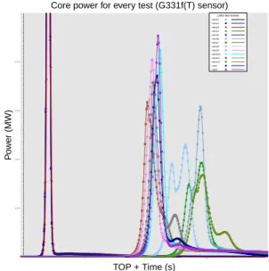
It is well known that we can have a lot of information only in observing data. And when we are able to work with a lot of data at the same time, it is powerfull to control the whole coherence apprehending available data for every test. With a language such as R, we easily superpose quantities as the experimental core power for every test (see figure 2). Graphics such as those of figure 3 and 4 are more powerful. On one diagram, the noise of every microphone given the test (see figure 3) is shown. The identical y-scale for all the diagrams yields important information about the acquisition system. Two tests ap-peared having a background noise with a high level. The work on dates can be controled thanks to a whole vision as in figure 4 juxtaposing available microphone values with the core power of every test.
Core power for every test (G331f(T) sensor)
TOP + Time (s) P o w er (MW) 1000 2000 3000 4000 0.2 0.4 0.6 ●●●●●●●●●●●●●●●●●●●●●●●●●●●●●●●●●●●●●●●●●●●●●●●●●●●● ● ● ● ● ● ● ● ● ● ● ● ●●●●●●●●●●●●●●●●●●●●●●●●●●●●●●●●●●●●●●●●●●●●●●●●●●●●●●●●●●●●●●●●●●●●●●●●●●●●●●●●●●●●●●●●●●●●●●●●●●●●●●●●●●●●●●●●●●●●●●●●●●●●●●●●●●●●●●●●●●●●●●●●●●●●●●●●●●●●●●●●●●●●●●●●●●●●●●●●●●●●●●●●●●●●●●●●●●●●●●●●●●●●●●●●●●●●●●●●●●●●●●●●●●●●●●●●●●●●●●●●●●●●●●●●●●●●●●●●●●●●●●●●●●●●●●●●●●●●●●●●●●●●●●●●●●●●● ●●●●●●●●●●●●●●●●●●●●●●●●●●●●●●●●●●●●●●●●●●●●●●●●●●●●●●●●●●●●●●●●●●●●●●●●●●●●●●●●●●●●●●●●●●●●●●●●●●●●●●●●●●●●●●●●●●●●●●●●●●●●●●●●●●●●●●●●●●●●●●●●●●●●●●●●●●●●●●●●●●●●●●●●●●●●●●●●●●●●●●●●●●●●●●●●●●●●●●●●●●●●●●●●●●●●●●●●●●●●●●●●●●●●●●●●●●●●●●●● ● ● ● ● ● ● ● ● ● ● ● ● ● ● ● ● ● ● ● ●● ● ● ● ● ● ● ● ● ● ● ● ● ● ● ● ● ● ●●●●●●●●●●●●●●●●●●●●●●●●●●●●●●●●●●●●●●●●●●●●●●●●●●●●●●●●●●●●●●●●●●●●●●●●●●●●●●●●●●●●●●●●●●●●●●●●●●●●●●●●●●●●●●●●●●●●●●●●●●●●●●●●●●●●●●●●●●●●●●●●●●●●●●●●●●●●●●●●●●●●●●●●●●●●●● ●●●●●●●●●●●●●●●●●●●●●●●●●●●●●●●●●●●●●●●●●●●●●●●●●●●●●●●●●●●●●●●●●●●●●●●●●●●●●●●●●●●●●●●●●●●●●●●●●●●●●●●●●●●●●●●●●●●●●●●●●●●●●●●●●●●●●●●●●●●●●●●●●●●●●●●●●●●●●●●●●●●●●●●●●●●●●●●●●●●●●●● ●●● ●● ● ● ● ● ● ● ● ● ● ● ● ● ● ● ●● ● ● ● ● ● ● ● ● ● ● ● ● ● ● ●●●●●●●●●●●●●●●●●●●●●●●● ●●●●●●●●●●●●●●●●●●●●●● ●●●●●●●●●●●●●●●●●●●●●●●●●●●●●●●●●●●●●●●●●●●●●●●●●●●●●●●●●●●●●●●●●●●●●●●●●●●●●●●●●●●●●●●●●●●●●●●●●
Liste des essais
repna1 repna2 repna3 repna4 repna5 repna6 repna7 repna8 repna9 repna10 repna11 repna12 cip01 cip02 ● ● ●
Figure 2: Core power for the studied CABRI tests The operations described so far are time consuming and often boring. Thus, already at the beginning of the work, it is preferable to be familiar with a programming scripting language to perform the different tasks which can be rerun and then useful to make the data consistent.
D. Creation of a catalogue of events
This step consists in proposing a global view of what happened during every test to the reader through the perception of the microphones. We had to manage:
1) The detection of events according to the signal-to-noise ratio,
3The TOP is the instant chosen by experimentalists to be the
Figure 3: Noise signal on the two microphones for every studied test
Figure 4: Core power and microphone signal available for every studied CABRI test
2) The storage of the events in a Relational Database, 3) The extraction of the events to propose an
visualiza-tion.
To detect an event, we used a sequential analysis tech-nique based on the moving variance of the signal. To decide the beginning and the end of an event we define a threshold from a learning set of values characteristic of the background noise (see figure 5). The algorithm is a little more complicated since we have to take into account the two microphones in the same time for the choice of the values t1 and t2. After detection, we store the values
of the two microphones and the values4 of two types of
flowmeters and pressure transducers. Finally, an event is defined by the signals of eight physical quantities.
There are presently stored in the database around one hundred events detected over the fourteen tests. The
4As the microphones, the flometers and the pressure transducers
are placed downstream and upstream from the test cell.
0.01 0.02 0.03 0.04 0.05 −6 −4 −2 0 2 4 6 Time (s) V oltage (V) Signal Moving Variance Time cut Sampling interval=1 µs Variance window = 500 Nb div/window = 50 Nbsigmas = 100 learning set noise threshold event duration t1 t2
Figure 5: Methodology used for the detection of an event
graphs of all events are inserted in the final report (see
figure 6 for the visualization of the event used to illustrate
the detection methodology).
Figure 6: Every event is caracterized by signal of several sensors
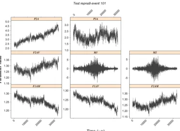
E. Pre-analysis
Once we completed the cleaning and the visualization of the data, we did the pre-analysis of the data which corre-sponds in fact to finding once again the results presented in the old technical report. This work consists in doing a descriptive analysis of the signals both in the time and frequency fields. Every event, we associated on the same graph (see figure 7):
• The value in time of the two microphones, the
pres-sure transducers and the flowmeters,
• The autocorrelation fonction, • The partial autocorrelation function, • The smoothed periodogram,
• The raw spectrum,
• The short-time Fourier Transformation.
Figure 7: Time and spectral analysis for every event Some specific signatures can be highlighted. That is the case for the events pertaining to the test shutdowns as shown on the short-time Fourier Transform in the bottom left corner of the figure 7. All these graphs are included in the final report. Here again, the Literate Programming offers a means to track the process precisely since we can keep the information about the methodology used to do the smoothing of the periodogram and the choice of parameters.
F. Statistical model
This section is about statistical modeling. This is the first time we have performed this task on our data. It is in fact the beggining of our ambition to carry out further investigations about the understanding of the physical phenomena appearing during the transient. For the mo-ment, the analysis has to be considered always as a part of tools to look at the data in order to have a better comprehension of our events.
So far, we observed the events only in the spectral do-main. Each of them is manipulated through its smoothed periodogram [12]. This one is divided in several bins as shown in figure 8 to create a vector with as many coordinates as number of bins. The figure 8 is an example with fifty bins but we took one thousand bins on the real data. Then, we performed a Correspondence Analysis [13]
to perform a dimensionality reduction. In term of vari-ability, this methodology allows us to define several new vectors, called factors, which retain a large part of the total variance from the initial space composed by the one thousand dimensions. In our case, we can work with ten factors to represent around eigthy percent of the total variance.
freq uency
V
2H
z
Every event is represented by a histrogram
50 classes for the plot, 1000 for the actual data
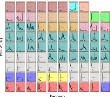
Figure 8: Methodology used for the detection of an event Then, a hierarchical clusthering [14] on these selected factors allows us to highlight twelve classes (see figure 9) typifying the shapes of periodograms (see figure 10).
Events stored in the Data Base
Agglomeration
criterion
85 86
12187 901248112282 88 83 84100 105 106 107 104 103 102 10865 96 61 62 641096311252 54 55 58 28 70 77 78 73 7911748 5311172 5111699 41 37 89 98115 11050 71 47 491258012691 3412033129 128 119 12332 46 97127 114 11327 94 31 95 2610144 45 39 38 40 42 35 36 29
Figure 9: The dendrogram
At this step, it would be possible to try to answer some questions such as, for example: "is there a relationship
between the core power average during an event and its frequency distribution". We begin to create a dependent
variable, that is to say a vector whose coordinates are the calculation of the core power mean value for each event (see red line in figure 11a). And we do a multiple linear regression, the independent variables being the selected factors 11b.
The previous analysis concluded that there is no sta-tistical relationship. In fact, there are some troubles in our data. For some classes, periodogram shapes point out the fact that we should have taken into account the low frequencies of the background noise for some tests (see figure 10 in the top left corner). Also, it would be better to work on the energy average instead of working on the core power average. In fact we must continue to prepare
Figure 10: The different shapes of periodograms
(a) Creation of the independent variable
(b) Multiple linear model
Figure 11: Questionning a linear relationship between the spectral contents and the average of the core power for each event
the data and then we enter into the cycle of iteration. V. Iteration
There are many reasons why we are obliged to return on the data processing:
• The initial raw data can change. During the data processing, we have to do physical assumptions which may be wrong,
• Change in the choices of the delay for dates in updat-ing,
• The abrupt changes detection algorithm can be im-proved, creating different events which would have a stronger physical meaning,
• According to the modifications of the previous steps,
we must be able to empty and populate the database with the new ones,
• The parameters can be set according to different
points of view leading to a trade-off,
• The background noise was not taken into account.
Using scripting languages rather than point-and-click to prepare the data and generate the final report, reconstruc-tion of results will then take only a few minutes. At every iteration, the coherence can be checked easily thanks to the global vision.
As explained in § II-B, all the tasks listed so far are placed in code chunks of the noweb file. But some of them can be time-consuming and we don’t want to repeat these tasks at every rerun. This situation is taken into account through the possibility of setting up options for every code chunk. Thus, when evaluating code chunks, we are able not to include some chunks in the global evaluation keeping the results of the previous runs. In order to give an idea of how it actually works, we propose a small example in the next section.
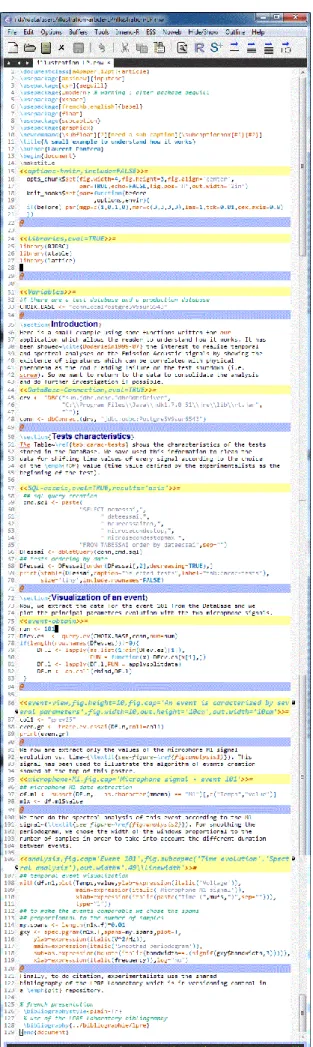
VI. A small example
We can see on the left side of the figure 12 the contents of a real noweb file which gives after compilation the document shown on the right part. The lines with yellow background mark the beginning of a code chunk. Every code chunk has a name. The @ lines with blue background mark the end of a code chunk and the beginning of a doc-umentation chunk. There is no name for a docdoc-umentation chunk. We can easily associate the results of the right part with the chunk of the left side. In the chunk "SQL-essais" we first make a request in the Database and then create the table. In the chunk "event-obtain", we access the data relative to event number 101 and we visualize it in the chunk "event-view". In the chunk "analysis", we do the smoothed periodogram calculation. We see that to make the events comparable we chose the spans proportional to the number of samples, thus resolution is identical for all events. In the header of a code chunk, with its name, we can add options as in the chunk "analysis" where we indicate the captions and the size of the figures. If we don’t want to evaluate this chunk at the next run, all we have to do is add an option as «analysis, eval=FALSE». This
approach is very flexible and it becomes easy to manage data processing from one file.
VII. Conclusion
The object of the work presented in this article was to put into action the strong links between the data, treatments and generation of the final technical report. According to the philosophy of the Literate Programming, the text of the technical document is mixed with the computer code that produces all the printed output such as tables, graphs for the study thereby eliminating the unrealistic point-and-click tasks. This difficulty is not specific to the nuclear field. For many years, researchers have worked out solutions to this mundane issue and presently, new technologies and high-level programming languages offer us actual answers. Applying this paradigm by ourself on our experimental data as explained, we can now say that Literate Programming can indeed become a reality. We have sought to make this article a teaser for experimentalists in encouraging them not to be afraid by the data driven analysis. From this work, we hope next time to be able to deduce interesting physical results.
Acknowledgment
The authors would like to thank the R core team and contributors for the creation and development of the R language and environment [5], which intelligently modified our way of doing experimental data processing.
References
[1] D. E. Knuth, “Literate programming,” Compt. J., vol. 27, no. 2, pp. 97–111, 1984.
[2] ——, The TEXbook. Addison-Wesley, 1984.
[3] ——, “The WEB system of structured documentation,” Stan-ford University, StanStan-ford, CA, StanStan-ford Computer Science Re-port CS980, Sep. 1983.
[4] N. Ramsey, “Literate programming simplified,” IEEE Softw., vol. 11, no. 5, pp. 97–105, Sep. 1994. [Online]. Available: http://dx.doi.org/10.1109/52.311070
[5] R Core Team, R: A Language and Environment for Statistical
Computing, R Foundation for Statistical Computing, Vienna,
Austria, 2014. [Online]. Available: http://www.R-project.org/
[6] F. Leisch, “Sweave and beyond: Computations on text
documents,” in Proceedings of the 3rd International Workshop
on Distributed Statistical Computing, Vienna, Austria,
K. Hornik, F. Leisch, and A. Zeileis, Eds., 2003, ISSN
1609-395X. [Online]. Available: http://www.R-project.org/
conferences/DSC-2003/Proceedings/
[7] Y. Xie, knitr: A General-Purpose Package for Dynamic Report
Generation in R, 2015, r package version 1.9. [Online].
Available: http://yihui.name/knitr/
[8] J. C. Faria, Resources of Tinn-R GUI/Editor for R
Environ-ment., UESC, Ilheus, Bahia, Brasil, 2012.
[9] RStudio Team, RStudio: Integrated Development Environment
for R, Boston, 2012. [Online]. Available: http://www.rstudio.
com/
[10] R. M. Stallman, “Emacs the extensible, customizable self-documenting display editor,” ACM SIGOA Newsletter, vol. 2, no. 1-2, pp. 147–156, Apr. 1981. [Online]. Available: http: //doi.acm.org/10.1145/1159890.806466
[11] S. Chacon, Pro Git. Apress, 2009.
[12] P. Bloomfield, Fourier Analysis of Time Series, J. WILEY and
I. Sons, Eds. John WILEY and Sons,INC, 2000.
[13] J. Benzécri, L’analyse des données: L’analyse des
correspon-dances, ser. L’analyse des données: leçons sur l’analyse
facto-rielle et la reconnaissance des formes et travaux. Dunod, 1973.
[14] G. Saporta, Probabilités, analyse des données et statistique. Editions Technip, 1990.
Figure 12: Contents of the noweb file illustration-LP.nrw on the left side and the result of the compilation on the right side, that is to say the file illustration-LP.pdf
![Figure 8: Methodology used for the detection of an event Then, a hierarchical clusthering [14] on these selected factors allows us to highlight twelve classes (see figure 9) typifying the shapes of periodograms (see figure 10).](https://thumb-eu.123doks.com/thumbv2/123doknet/12950503.375854/6.918.79.464.220.590/methodology-detection-hierarchical-clusthering-selected-highlight-typifying-periodograms.webp)