Navigating Wikipedia with the Zoomable Adjacency Matrix Explorer

HAL Id: inria-00141168

https://hal.inria.fr/inria-00141168v3

Submitted on 24 Apr 2007

HAL is a multi-disciplinary open access

archive for the deposit and dissemination of

sci-L’archive ouverte pluridisciplinaire HAL, est

destinée au dépôt et à la diffusion de documents

Matrix Explorer

Jean-Daniel Fekete, Niklas Elmqvist, Thanh Nghi Do, Howard Goodell,

Nathalie Henry

To cite this version:

Jean-Daniel Fekete, Niklas Elmqvist, Thanh Nghi Do, Howard Goodell, Nathalie Henry. Navigating

Wikipedia with the Zoomable Adjacency Matrix Explorer. [Research Report] RR-6163, INRIA. 2007,

pp.25. �inria-00141168v3�

inria-00141168, version 3 - 24 Apr 2007

a p p o r t

d e r e c h e r c h e

Navigating Wikipedia with the Zoomable Adjacency

Matrix Explorer

Jean-Daniel Fekete — Niklas Elmqvist — Thanh-Nghi Do — Howard Goodell — Nathalie

Henry

N° 6163

Matrix Explorer

Jean-Daniel Fekete , Niklas Elmqvist , Thanh-Nghi Do , Howard Goodell ,

Nathalie Henry

Th`eme COG — Syst`emes cognitifs Projet AVIZ

Rapport de recherche n°6163 — 2007 — 25 pages

Abstract: This article presents the Zoomable Adjacency Matrix Explorer (ZAME), a

visualization tool for exploring networks at a scale of millions of nodes and tens of millions of edges. ZAME presents an adjacency matrix graph representation aggregated at multiple scales. It allows analysts to explore a graph at many levels, zooming and panning with interactive performance from the most summary to the most detailed views.

Several components work together to make this performance possible and the results meaningful. A “pyramid” of aggregated views paged on demand to OpenGL GPU shader programs supports smooth multiscale browsing in huge datasets. Efficient matrix ordering algorithms group related elements to make the views meaningful. Using ZAME, we can ex-plore the entire French Wikipedia, over 500,000 articles and 6,000,000 links, with interactive performance on standard consumer-level computer hardware.

Key-words: Large-scale graph visualization, matrix-based representation, node-link dia-grams, multi-scale navigation, matrix ordering, graph aggregation.

∗

R´esum´e : Cet article d´ecrit l’Explorateur de Matrice d’Adjacence Zoomable (ZAME), un outil de visualisation destin´e `a explorer des r´eseaux de l’ordre d’un million de nœuds et de dix millions d’arˆetes. ZAME montre le graphe sous la forme d’une matrice d’adjacence agr´eg´e en plusieurs niveaux. Il permet `a un analyste d’explorer un graphe `a tous les niveaux et zoomant et d´epla¸cant la vue de mani`ere totalement interactive de la vue la plus r´esum´ee `

a la vue la plus d´etaill’ee.

Plusieurs composant sont coupl´es pour donner ces performances et rendre la repr´esentation intelligible: une Pyramide de vues agr´eg´ees, pagin´ees et envoy´ees `a l’´ecran `a la demande `a travers un programme utilisant les Shaders programmables d’OpenGL. Tous ces m´ecanismes permettant une exploration rapide et continue de masses de donn´ees. Des algorithmes de r´eordonnancement de matrice permettent de rendre cette repr´esentation compr´ehensible. En utilisant ZAME, nous pouvons explorer interactivement et sur une machine multim´edia standard la totalit´e de l’hypertexte que constitue la version fran¸caise de Wikipedia, constitu´ee de plus de 500 000 articles et de 6 000 000 de liens.

Mots-cl´es : Visualization de graphe de grande taille, repr´esentation matricielle, diagramme nœud et lien, navigation multi-´echelle, r´eordonnancement de matrice, agr´egation de graphe.

1

Introduction

Few Internet users today are unaware of the Wikipedia online encyclopedia project. Written exclusively by volunteers on the Internet, Wikipedia has become the ninth most popular site on the Web since its inception in 2001. As of this writing, its versions in 250 languages contain more than six million articles, over 1.6 million in the English version alone, making it the largest encyclopedia ever assembled. Most users of Wikipedia today read individual articles or series of articles as in a traditional encyclopedia. However, some users would like to view and analyze the collection as a whole, such as Wikipedia administrators or sociology researchers who want to study its structure and connectivity.

If this can be done easily, more-typical Wikipedia readers might be able to profit from a graphical overview showing where the articles they have read fit in a grouping of related articles. These overviews might include visual clues about the character of the article to help them decide where to go next, such as article length, number of accesses or citations, update activity, authorship, or perhaps rating by some future online editorial agency that the reader trusts. Such tools could enable whole new patterns of exploration that many people will use to study Wikipedia.

This pattern is not limited to Wikipedia, but is part of two general trends. Increasingly, analysts in many fields need to explore and understand large, complex networks with mil-lions of vertices and milmil-lions or billion of edges. Also, where appropriate tools have been developed, ordinary users with personal computers today explore datasets on grand scales— the geography of our entire planet, or all the stocks of the New York exchange—that until recently were the domain of specialists.

For example, we are collaborating with sociologists seeking to understand the dynamics of large online social networks. The social network of the Wikipedia project links tens of thousands of writers to hundreds of thousands or millions of articles; open-source software projects such as the Debian Linux distribution link hundreds of developers to thousands of software modules. Currently they have only statistical tools to test their models of these networks, because interactively exploring such large networks remains a challenge for existing information visualization tools.

In this article, we present the Zoomable Adjacency Matrix Explorer (ZAME), the first system that permits meaningful visual navigation of the whole of Wikipedia, from an overview of the entire corpus down to the individual articles, seamlessly and with interactive performance. ZAME is based on a zoomable multiscale adjacency matrix representation of Wikipedia articles and their internal links. It implements three original features:

ˆ a fast automatic reordering mechanism to find a good layout;

ˆ special indices supporting a rich variety of data aggregations; and

ˆ GPU-accelerated rendering with programmble shaders to deliver interactive and smooth

framerates.

ZAME can be used with any network including social networks and bioinformatics net-works. The system provides two different scales of zoom—geometric zoom as well as detail

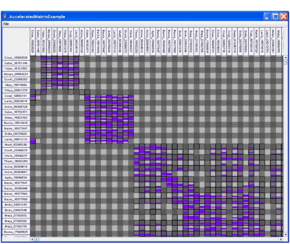
Figure 1: Screenshot of ZAME showing a min-max aggregation of numerical values. zoom—allowing the user to independently change both the amount of data visible on the screen as well as the size allocation of each data point. In addition, we use special visual rep-resentations of aggregated edges implemented in shader programs to make the aggregation (and its contents, if desired) evident to the user.

The remainder of this article is organized as follows: we first present a survey of related work. This is followed by a description of ZAME’s features and design. We conclude with a discussion of its current implementation and performance results.

2

Related Work

The most crucial attribute of a graph visualization is its readability, its effectiveness at conveying the information required by the user tasks [11]. For example, Ghoniem et al. pro-posed a taxonomy of graph tasks and evaluated the effectiveness of node-link and adjacency matrix graph representations to support them in [17]. They found that graph visualization readability depends strongly on the graph’s size (number of nodes and edges) and density (average edges per node). Different visualizations had better readability for different graph sizes and densities, as well as for different tasks.

Several recent efforts visualize large graphs with aggregated representations that present node-link and/or matrix graphs at multiple levels of aggregation. The following sections describe several important ones.

2.1

Node-Link Visualization of Large Networks

Node-link diagrams can effectively visualize networks of about one million vertices if they are relatively sparse. Hachul and J¨unger [14] compared six large-scale graph drawing algorithms for 29 example graphs, some synthetic and some real, of which the largest had 143,437 vertices and 409,593 edges. Of the six algorithms, only three scaled well: HDE [15], FM3

[13] and to some extent GRIP [9]. However, the densities of the sample graphs were small, typically less than 4.0. When the density or the size grows, some dimensionality reduction mechanism is needed to maintain readablity.

Hierarchical aggregation allows larger graphs to be visualized and navigated, assuming that there is an algorithm for finding suitable aggregations at each level in a reasonable time. An aggregation is suitable if each aggregated level can be visualized effectively as a node-link diagram, and if navigation between levels has sufficient visual continuity for users to maintain their mental map of the whole network and avoid getting lost. No automated strategy published to date can select an appropriate algorithm for an arbitrary network, but there are many successful aggregation algorithms for specific categories of graphs. For example, Auber et al. [3] present effective algorithms for aggregating and visualizing the important class of networks (including the global Internet and many social networks) known as small-world networks [20], whose characteristics include power-law degree distribution, high clustering coefficient and small diameter. Systems such as Tulip offer multiple clustering algorithms and are designed to permit smooth navigation on large aggregated networks [2]. Gansner et al. propose another method involving a topological fisheye that is usable when a correct 2D layout can be computed on a large graph [10]. After the network is laid out, it is topologically simplified to reduce the level of detail at coarser resolutions. The fisheye selects a focus node and displays the full detailed network around it, showing the remainder of the network at increasingly coarse resolutions for nodes farther away from the focus. This technique preserves users’ mental maps of the whole graph while magnifying (distorting) the network around the focus point. However, effectively laying out an arbitrary large, dense graph remains an open problem for node-link diagrams. All the methods require a good global initial layout, which can be very expensive to compute.

Wattenberg [19] describes a method for aggregating networks according to attributes on their vertices. The aggregation is only computed according to the attribute values, much like pivot tables in spreadsheet calculators or data cubes in OLAP databases. This approach works best when the values are categorical or numerical with a low cardinality. The article only refers to categorical attributes on the vertices. When no categorical attribute is suitable for computing the pivots, as with the Wikipedia hypertext link network visualized in this paper, this approach is not effective—the whole network would be displayed as a single point.

Overall, the node-link representation has two major weaknesses [11]: (i) it copes poorly with dense networks, and (ii) without a good layout, it requires aggregation methods to reduce the density enough to be readable. Because these methods are very dataset depen-dent, current node-link visualization systems leave the choice of aggregation and layout to the users, who therefore need considerable knowledge and experience to get good results.

2.2

Matrix Visualization of Large Networks

Several recent articles have used the alternative adjacency matrix representation to visualize large networks. Abello and van Ham demonstrated [1] the effectiveness of the matrix rep-resentation coupled with a hierarchical aggregation mechanism to visualize and navigate in networks too large to fit in main memory. Their approach is based on the computation of a hierarchy on the network displayed as a tree in the rows and columns of the aggregated ma-trix representation. The aggregation is a hierarchical clustering in which items are grouped but not ordered. It is computed according to memory constraints as well as semantic ones. The users operate on the tree to navigate and understand the portion of the network they are currently viewing.

Navigation in this approach is constrained by the hierarchical aggregation: users navigate in a tree that has been computed in advance. The main challenge is to find an aggregation algorithm that is both fast and that produces a hierarchy meaningful to the user. Unfor-tunately, this choice is typically dataset-dependent. Without a meaningful hierarchy, users navigate in clusters containing unrelated entries and cannot make sense of what they see.

Henry and Fekete in [16] proposed several methods based on reordering the rows and columns of the matrix as opposed to just clustering similar nodes. They describe two methods based on approximate Traveling Salesman Problem (TSP) solutions, which are computed on the similarity of connection patterns and not on the network itself. One method uses a TSP solver directly; the other initially computes a hierarchical clustering and then reorders the leaves using a constrained TSP. Both algorithms yield orderings that reveal clusters, outliers and interesting visual patterns based on the roles of vertices and edges. Because the matrix is ordered, not just clustered, both navigation (panning) between and within clusters of similar items may reveal useful structure. Unfortunately, both reordering methods are at best quadratic; since they need to compute the full distance matrix between all the vertices. Therefore, it is difficult to scale them to hundreds of thousands or millions of vertices.

Interactive System Representation Data Reordering Automatic Graph Database Visualization Navigation

Figure 2: Overview of the components of ZAME.

3

The Zoomable Adjacency Matrix Explorer

ZAME is a network visualization system based on a multiscale adjacency matrix representa-tion. Attributes associated with the vertices and edges can be mapped to visual attributes of the visualization, such as color, transparency, labels, border width, size, etc., using se-lectable schemes to aggregate each attribute appropriately at higher levels. ZAME integrates all the views of a large network, from the most general overview down to the details, and provides multiscale navigation techniques that operate at all levels. Therefore, it can be used for tasks at all levels, from understanding the network’s overall structure, to exploring the distribution of results to a content-based search query at multiple levels of aggregation, to performing analysis tasks such as finding cliques or the most central vertices. Additional relevant graph tasks can be found in [17].

The main technical challenge of the system is managing the huge scale of such graphs— on the order of a million vertices for the Wikipedia database—while delivering the real-time framerates necessary for smooth interaction. Furthermore, the graph must be laid out (the matrix nodes reordered) to group similar nodes so that the visualization becomes readable, i.e. in such a way that patterns emerge and conclusions can be drawn from the data.

To achieve these goals, our tool consists of four different components (see Figure 2):

ˆ a hierarchical data structure for storing the graph and its attributes in an aggregated

format;

ˆ an automatic reordering component for computing a meaningful order for the matrix

to support visual analysis;

ˆ an accelerated rendering mechanism for efficiently displaying and caching a massive

graph dataset; and

ˆ a set of navigation techniques for exploring the graph.

3.1

Multiscale Data Aggregation

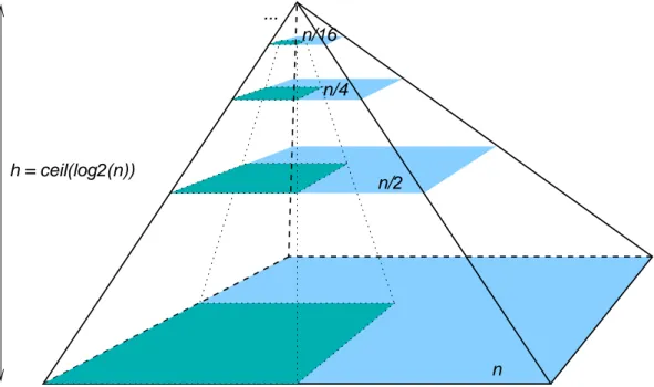
To support multiscale graph exploration with interactive response, we designed an index structure tailored to its visualization abstraction, the 3-dimensional binary pyramid of “de-tail levels” shown in Figure 3. Users pan across the surface of one de“de-tail level; they zoom up and down between detail levels (along perspective lines meeting at the tip of the pyramid, so features match between zoom levels). Detail level zero of this abstraction, the bottom level of the pyramid, is the adjacency matrix of the raw data with the nodes arranged (according to the reordering permutation) on the rows and columns at the edge and the edges between them indicated at the row/column intersections on the level’s surface. Every detail level above the base has half the length and width (number of nodes) and a quarter the intersec-tion squares (possible edges) as the level below it. Therefore, each node at a higher, more summary detail level represents two nodes at the level below it (except the last node on a level, in the case where the lower level had an odd number of nodes), and each intersection square indicating a possible edge at this level represents four possible edges at the level below it.

Combining nodes and edges for higher detail levels require that we define how to aggre-gate the underlying data and its corresponding visual representation. See Sections 3.3 and 3.5 for these definitions.

n/16

n/4

n/2

...

n

h = ceil(log2(n))

3.1.1 Pyramid Index Structure

The original network at detail level 0 is stored as a standard graph in the InfoVis Toolkit (IVTK) [7]. The specialized index structure is maintained in “zoomable” equivalents spe-cialized for the pyramid index structure.

A standard IVTK graph is implemented by a pair of tables, one for its vertices and another for its edges. Each row represents one vertex or edge. It contains attributes in “internal columns” that maintain the graph topology. For each vertex, there is a first and last edge for each of two linked edge lists for its outgoing and incoming edges. Each of these lists is maintained in a pair of columns in the edge table: the “next edge” and “previous edge” for the outgoing and incoming edge lists. To complete the topology, two more columns of the edge table store its first and second vertex (source and sink edge vertices for directed graphs). The doubly-linked edge lists are an optimization for fast edge removal, but the back-link can be omitted to reduce memory consumption if necessary. Thus, the IVTK needs to store four numbers for each vertex, and either six or four numbers for each edge. Its current implementation uses CERN COLT [6] primitive integer arrays that have very little overhead; so in a 32-bit Java implementation today, the memory consumed is 16 bytes for each vertex and 16-24 bytes for each edge.

A zoomable graph has the same basic structure. However, instead of single-layer vertex and edge tables, it uses specialized “zoomable” tables with multilevel indices. Also, it maintains some invariants that accelerate important operations. Below is a description of the basic operations:

getRelatedTable() returns the original table the zoomable table aggregates;

getItemLevel(int item) returns the aggregation level for a specified item, 0 for the orig-inal level and ⌈log2(|V |)⌉ for the highest level with only one element, |V | being the

number of vertices of the graph;

getSubItems(int item) returns a list of items in the next lower aggregation level (two vertices or up to four edges);

getSuperItem(int item) returns the corresponding item at the next higher aggregation level; and

iterator(int level) returns an iterator over all the elements of a specified aggregation level.

The zoomable vertex table refers to the original graph’s vertex table (its related table.) Each aggregated vertex at level 0 refers to one vertex in the related table, except that their order is changed by a “permutation” structure that implements the reordering described in 3.2. The numbering of aggregated vertices at level 1 begins immediately after those at level 0, 2 after 1, and so forth (except that an odd number at any level is rounded up by one). Each pair of vertices at at level n is aggregated by a single vertex at level n + 1. So, given the number of a vertex at any level, this simple numbering scheme makes it straightforward

to compute corresponding vertices at levels above and below it. It is also straightforward to calculate the size of the index: it is bounded by the series 1/2+1/4+. . . < 1; so all the index levels at most double the size of the table. Like vertices at level 0, an aggregated vertex has pointers (edge numbers) to its lists of out- and in-edges, but these refer to aggregated edges. Unfortunately, the zoomable edge table index is much more complicated to build and maintain, because the set of possible edges is not dense. The number of possible edges between N nodes is on the order of N2

; so in 32-bit signed arithmetic, calculations based on a simple enumeration of possible edges analogous to those used for vertex indices would overflow for more than 215

(32K) vertices. As with the vertex table, edges at level n follow edges at level n − 1. However, because the corresponding edge numbers at each level cannot be calculated, they must be stored. Achieving fast access requires several optimizations. To compute the level of an edge, we perform a binary search in a vector containing the starting index of each level. At each level, the outgoing edges are stored in order by their first (source) vertex: the outgoing edges of vertex n follow the outgoing edges of vertex n−1. Similarly, all the outgoing edges for one source vertex are sorted in order of their second (sink) vertex. This arrangment makes it very fast to search for an edge given its vertices using two levels of binary search. This optimization allowed us to omit the previous and next edge columns for aggregated edges.

Despite memory optimizations such as using binary search in edge lists ordered at two levels to replace next-edge and previous-edge lists, aggregated edge indices are still very costly in terms of memory, several times larger than the original data. We still need to maintain a separate incoming edge list. We also need an extra column to store the “super edge” (that is, the corresponding edge in the level above). This appears wasteful; since the “super vertex” corresponding with this endpoint could be calculated and the super edge found by a binary search in the edge list of the super vertex. Wikipedia has around six million edges; so 24 Mb are required just to add this one column to the base level, and the total including all its index levels is around five times more. However, we still chose to store this information, because the basic operation of aggregating edge attributes requires going through each edge from level 0 up and accumulating the aggregated results on the super edge. Without direct access, the complexity of this operation would be n × log(n) instead of n, and it would require tens of minutes instead of minutes.

Because the amount of information used for aggregated indices on a huge file such as Wikipedia exceeds the virtual memory capacity of a 32-bit Java Virtual Machine (JVM), we implemented a paging mechanism that allocates columns of memory in fairly large fixed-size chunks that are retrieved from disk when needed. Fortunately, the memory layout of the zoomable aggregated graph is very well suited to paging. Most operations are performed in vertex- and edge-order on a specified level; so they tend to use consecutive indexes likely to be allocated nearby on disk.

The total size of the aggregated edge table depends dramatically on the quality of the ordering. A good ordering groups both edges and non-edges; so multiple nearby edges and non-edges aggregate at each step and the size of successive index levels rapidly diminishes. The worst case is a “pepper and salt” pattern of widely-spread edges that do not aggregate

significantly for many levels, resulting in an aggregated edge table that can be 4 to 8 times larger than the original edge table. Because Wikipedia averages only 12 links per page, without a good ordering it has this kind of profile. Our current reordering methods, though imperfect, improve this to about a factor of 5.

3.2

Reordering

Of all the algorithms described in the literature on matrix reordering, few are sub-quadratic. We experimented with those based on linear dimension reduction such as Principal Compo-nent Analysis (PCA) or Correspondance Analysis (CA) and greedy TSP algorithms such as the Nearest-Neighbor TSP (NNTSP) heuristic.

3.2.1 High-Dimensional Embedding

PCA and Correspondence Analysis were used effectively by Chauchat and Risson [5] for reordering matrices. Their matrices were small enough to permit computing the eigenvectors directly, but this is obviously infeasible for hundreds of thousands or millions of points. Harel and Koren describe a modified PCA method called “High Dimensional Embedding” [15] that can efficiently lay out very large graphs by computing only k-dimensional vectors where k is typically 50. This method is designed for laying out node-link diagrams by using the two or three first components of the PCA for positioning of the vertices. We used it and improved it for reordering matrices.

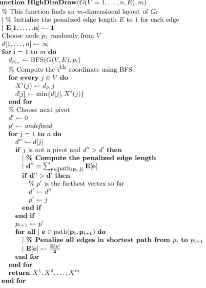
The solution proposed by Harel and Koren consists of choosing a set of pivot vertices that the algorithm tries to place near the outer edges of the graph, and to use the graph distances to these pivots as the coordinates of each vertex. When 50 pivots are chosen, these coordinates are in 50 dimensions. PCA is computed on these dimensions and the eigenvectors are computed using a power-iteration that converges very quickly in real cases. Their main algorithm is listed in Figure 9. The BFS algorithm is a simple Breadth First Search computed when no edge weights exist; otherwise, it is replaced by a Dijkstra shortest path computation.

Figure 4) compares the results of HDE versus TSP on a relatively small social network dataset. Although HDE’s results (right side) are noticeably worse, the calculation is much faster, requiring just a fraction of second instead of 30 seconds required by the standard TSP solver that produced the figure on the left. Although the TSP solver clearly could not be applied to the far larger Wikipedia dataset, HDE reordering is quite fast, but again, the local quality of the ordering is poor.

More seriously, the original algorithm can choose pivots in a very ineffective way. Con-sider a large connected network with two very distant star-shaped vertices V1and V2, much

more distant than any other vertices except the children of these two vertices. HDE will pick a random pivot first, then take the farthest vertex from the pivot, say around V1. The next

vertex will then be a pivot around V2. In turn, the next will be another vertex around V1

etc. until all the children of V1and V2 are enumerated, producing a very biased distribution

Figure 4: Results of the algorithms TSP (left) and HDE (right) applied to a social network occurs in Wikipedia. Because the taxonomies of the animal and plant kingdoms in biological species classifications are the deepest tree structures in Wikipedia, unmodified HDE merely enumerates the deepest leaves of these two classifications. Obviously major axes determined by PCA of this highly unbalanced node selection will not represent the rest of Wikipedia.

00

00

11

11

00

00

11

11

00

11

00

11

0

0

1

1

00

11

₀

0

₁

1

0

1

0

0

1

1

00

11

0

1

00

11

00

11

00

11

00

11

00

11

00

11

00

11

₀₀

00

₁₁

11

00

00

11

11

0

0

1

1

00

11

0

0

1

1

00

11

0

10

1

0

1

0

0

1

1

00

11

0

10

10

1

0

1

00

11

00

11

0

1

00

00

11

11

00

00

11

11

0

0

1

1

0

0

1

1

0

1

0

1

0

1

0

1

0

1

0

1

00

11

0

1

00

11

00

11

00

00

11

11

0

0

1

1

00

00

11

11

00

00

11

11

00

11

0

0

1

1

00

00

11

11

00

11

00

11

0

1

0

1

00

00

11

11

00

11

0

1

0

0

1

1

00

00

11

11

0

0

1

1

0

0

1

1

0

1

0

0

1

1

0

0

1

1

00

11

0

0

1

1

00

00

11

11

0

0

1

1

0

0

1

1

0

1

0

1

00

00

11

11

00

11

0

1

0

0

1

1

0

0

1

1

0

0

1

1

00

00

11

11

2

1

0

1

0

0

0

0

1

1

1

1

00

00

11

11

Figure 5: Pathological HDE pivot selection for the Wikipedia dataset.

To avoid this bias, we modified HDE to penalize edges progressively according to the number of times they already participate in a path between existing pivots (Figure 9). This penalty encourages the algorithm to place new pivots in regions of the graph not traversed

by paths between previous pivots, which hopefully represent important different features of its overall structure.

This algorithm avoids the pathological distribution of pivots, but it does not solve the fundamental question of how many pivots are required to adequately represent a large graph, which is still an open question.

3.2.2 Nearest-Neighbor TSP Approximation

Although the Traveling Salesman Problem is NP-complete, it has good approximations in many cases. When the edges are weighted and the weight values are not too similar, the Nearest-Neighbor TSP (NNTSP) approximation algorithms can be can be effective [12]. An initial ordering can be computed in linear time by limiting the search distance. In our NNTSP algorithm we limit the distance to 6 since the number of nodes examined grows by a factor of 12 (the average number of links per page in Wikipedia) on each iteration, and we felt that pages more than 6 hops away were unlikely to be good matches.

Because hypertext links are unweighted, we computed various dissimilarity functions between the source and destination pages of the link to provide them.

To date, we have tried three link-weighting or distance-calculation algorithms. In order of increasing quality and running time, they are dissimilarity of adjacency patterns, distance in the HDE pivot space and distance in a randomly-selected pivot space. (Dis)similarity of adjacency patterns is determined by merging the set of destination vertices between the edge sets of a pair of source vertices. Visually, an ordering that optimizes this measure will tend to maximize the number of groups of aligned squares on an adjacency matrix representation, which is good for perceptual analysis. This measure can be calculated efficiently—in time linear in the average number of vertices per node—so it was the first one we tried.

NNTSP using this distance measure does a reasonable job of aligning almost all the vertices of Wikipedia—about 97%, approximately the first 460,000 of the 474,594 pages in its largest connected component that we actually analyze (since graph distance cannot be computed for unconnected components). However, at the end of the NNTSP algorithm, when relatively few unvisited vertices remain to be placed, the chance of finding pages with common links is small. Therefore, since the adjacency pattern measure is likely to be zero for all of the remaining pages, even when it is computed for neighbors of neighbors of neighbors . . . many cannot discriminate between them and the search for a match becomes very long. The second and third methods we tried differ from the first by the adjacency pattern dissimilarity metric. First, they find some number (currently 10) of HDE pivots, respectively either by Harel and Koren’s method [15] or randomly. They compute the distances between every graph point and each pivot, which takes about 20 seconds per pivot for Wikipedia. Then, each graph distance is approximated by the Triangle Inequality: the true distance between vertices is less than the sum of the distances between the two vertces and any pivot. The shortest distance is used (corresponding to the closest pivot). Dissimilarity is computed on the distance-to-pivots coordinate space and nearest-neighbor is also computed in that space. These methods find better orderings for the graph than the first (which gives

up and accepts a low-quality ordering for the last 3% of the points) at the expense of several minutes longer calculation time.

3.2.3 Results

The HDE method provides the best overview of the graph at a high, heavily-aggregated level, with the majority of connected nodes grouped in the upper left corner. In contrast, the NNTSP algorithm orders the Wikipedia data reasonably well globally, but dramatically better locally. The global order is actually not as good as HDE’s, as reflected by a poorer compression factor of the indicesd—NNTSP leaves more “salt and pepper” vertices. How-ever, its ordering is dramatically better at a small scale. Basically, it finds many large groups of closely-related pages, groups them in the order and arranges them reasonably. It is the default reordering method we apply.

We provide some examples of the reordering performance of the three algorithms pro-posed in this paper to show the difference in results on both global as well as local level. See Figure 10 for overview and detail views of the results of reordering the same matrix using the HDE, NNTSP, and NNTSP2 algorithms.

3.3

Aggregating Data Attributes

To make views of data at a higher level meaningful, attributes of the original vertices (such as article names, creation date, or number of edits) and edges (such as link weights) must be combined in meaningful ways, with rapid access to details including the original data values. This requires considerable flexibility in order to accommodate a range of data types and semantics as well as user intentions. There is a new trend in the classification community to use so-called “symbolic data analysis” for richer aggregation [4]. We summarize the principle and explain how we map symbolic data to visualizations.

It is important to make it evident to the user when a particular cell is representing an aggregated, as opposed to an original, attribute. Section 3.5 describes some of the visual representations we employ for this purpose. Typically, if enough display space is available, a histogram can faithfully visualize the aggregated values for each item. If less space is available, a min/max range or Tukey diagram can be used. In the worst case, where only one or a few pixels are available, the aggregated value can be used to modulate the color shade of the whole cell.

3.3.1 Categorical Attributes

Categorical attributes—including Boolean values—have a cardinality: the number of cate-gories. At the non-aggregated level, a categorical variable can hold one categorical value, such as a US state. When aggregating categorical values, we compute a distribution, i.e. the count of each item aggregated per category.

3.3.2 Numerical Attributes

Numerical attributes may be aggregated by various methods such as mean, maximum or minimum. They can also be transformed into categorical values by binning the values in intervals. Numerical data permits a wide range of analysis such as calculating standard deviations and other statistics. ZAME internally computes a discrete distribution for the aggregated values using a bin width computed according to [18]. We also keep track of the mean, extreme, and median values.

3.3.3 Nominal Attributes

Unlike even ordinal data, there is no inherent relationship between nominal attributes such as article names, authors, or subject titles. Unfortunately, they are often vital to understand-ing what elements of the visual representation refer to. Like numeric attributes, nominal attributes of specific datasets can be aggregated using special methods such as concatena-tion, finding common words, or sampling representative labels. Methods such as excentric labels [8] may be used to display many more labels on demand.

3.4

Visualization

For the visualization component of our matrix navigation tool, we are given an elusive challenge: to efficiently render a matrix representation of a large-scale aggregated graph structure consisting of thousands if not millions of nodes and edges. The rendering needs to be efficient enough to afford interactive exploration of the graph with a minimum of latency. We can immediately make an important observation: for matrices of this magnitude, it is the screen resolution that imposes a limitation on the amount of visible entities. In other words, there is no point in ever drawing entities that are smaller than a pixel at the current level of geometric zoom. In fact, the user will often want the entities to be a great deal larger than that at any given point in time. This works in our favor and significantly limits the depth we need to traverse into the aggregated graph structure in order to render a single view of the matrix.

At the same time, we must recognize that accessing the aggregated graph structure may be a costly operation and one which is not guaranteed to finish in a timely manner. Clearly, in order to achieve real-time framerates, we must decouple the rendering and interaction from the data storage.

Our system solves this problem by utilizing a tile management component that is re-sponsible for caching individual tiles of the matrix at different detail levels. Missing tiles are temporarily exchanged for coarser tiles of a lower detail level until the correct tile is loaded and available. The scheme even allows for predictive tile loading policies, which try to predict user navigation depending on history and preload tiles that may be needed in the future.

In the following text, we describe these aspects of tile management and predictive loading in more depth. We also describe our use of programmable shaders and textures for efficiently rendering matrix visualizations.

3.4.1 Basic Rendering

Instead of attempting to actively fill and stroke each cell representing an edge in our ad-jacency matrix, we use 2D textures for storing tiled parts of the matrix in video memory. Textures are well-suited for this purpose since they are regular array structures, just like ma-trix visualizations. Also, they are accessible to programmable vertex and fragment shaders running on the GPU (graphical processing unit) of modern 3D graphics cards. This allows us to avoid sending excessive geometry data to the GPU and instead render a few large triangles with procedural textures representing the matrix.

Our basic matrix rendering shader accesses the texture information for a given position and discards the fragment if no edge is present. If there is an edge there, the data stored in the texture is used to render a color or visual representation (see Section 3.4.1). Stroking is performed automatically by detecting whenever a pixel belongs to the outline of the edge—in this case, black is drawn instead of the color from the visual representation of the edge.

3.4.2 Tile Management

Adjacency matrices may represent millions of nodes on a side, and thus storing the full matrix in texture memory is impossible. Rather, we conceptually split the full matrix into tiles of a fixed size and focus on providing an efficient texture loading and caching mechanism for individual tiles depending on user navigation.

In our implementation, we preallocate a fixed pool of tiles of a given size. We use an LRU cache to keep track of which tiles are in use and which can be recycled. As the user pans and zooms through the matrix, previously cached tiles can be retrieved from memory and drawn efficiently without further cost. Tiles which are not in the cache must be fetched from the aggregate graph structure—this is done in a background thread that keeps recycling and building new tiles using the cache and the tile pool.

While an unknown tile is being loaded in the background thread, the tile manager uses an imposter tile. Typically, imposter tiles are found by stepping upwards in detail zoom levels until a coarser tile covering the area of the requested tile is eventually found in the cache. The imposter is thus an aggregation of higher zoom levels and therefore not a perfectly correct view of the tile, but it is sufficient until the real tile has finished loading.

3.4.3 Predictive Tile Loading

Beyond responding to direct requests from the rendering, our tile caching mechanism can also attempt to predictively load tiles based on an interaction history over time. For example, if the user is increasing the detail zoom level of the visualization, we may try to preload a number of lower-level tiles in anticipation of the user continuing this operation. Alternatively,

Tile LRU cache manages OpenGL Rendering Pipeline Transformation Vertex ... Coloring Fragment Rendering: geometry data 0011101011001 0101101101110 0101101101110 matrix visualization fragment shaders Screen ... Tile TileManager contains paint(mCoords, wCoords) owns OpenGL textures ... ... edge values ... tracks

coords, zoom : int queries

programmable components TileProvider

loadTile(cs, zoom)

Figure 6: Matrix visualization rendering pipeline.

if the user is panning in one direction, we may try to preload tiles in this direction to make the interaction smoother and more correct.

Our tile manager implementation supports an optional predictive tile loading policy that plugs into the background thread of the tile manager. Depending on the near history of requested tiles, the policy can choose to add additional tile requests to the command queue. Furthermore, the visualization itself can give hints to the policy on the user’s interaction.

3.5

Aggregated Visual Representations

By employing programmable fragment shaders to render procedural textures representing matrix tiles, we get access to a whole new set of functionality at nearly no extra rendering cost. In our system, we use this capability to render special visual representations for aggregated edges. As indicated in Section 3.3, we can use these to give the user an indication of the data that has been aggregated to form a particular edge.

Currently, we support the following such visual representations (see Figure 7 for examples of these):

ˆ Standard color shade. Single color to show occupancy, or a two-color ramp scale

to indicate the value.

ˆ Average. Computed average value of aggregated edges shown as a “watermark”value

Figure 7: Seven different visual representations for aggregated edges.

Cell edge detection

2−color ramp function OpenGL color

fragment color output

shader input:

(for stroking)

Matrix edge detection Aggregate Visual_{Representation}

(depends on shader)

discard

no edge stroke: black outside: white

entry

Figure 8: Schematic overview of a matrix visualization fragment shader.

ˆ Min/max (histogram): Minimum and maximum values of aggregated edges shown

as a smooth histogram.

ˆ Min/max (range): Minimum and maximum values of aggregated edges shown as a

color range.

ˆ Tukey box: Average, minimum and maximum values of aggregated edges shown as

Tukey-style lines.

ˆ Histogram (smooth): Four-sample histogram of aggregated edges shown as a smooth

histogram.

ˆ Histogram (step): Four-sample histogram of aggregated edges shown as a bar

his-togram.

Each representation has been implemented as a separate fragment shader and can easily be exchanged. Furthermore, new representations can also be added. Depending on the avail-ability and interpretation of the data contained in the tile textures, the user can therefore switch between any of these representations at will and with no performance cost.

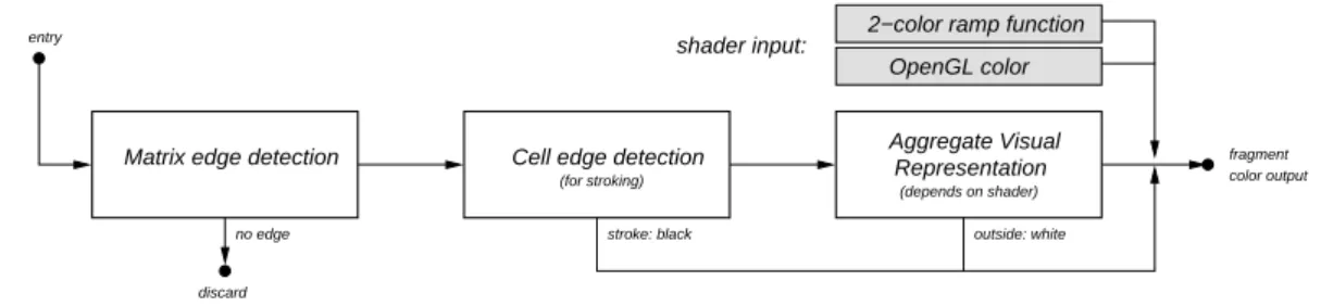
Figure 8 shows a general overview of the fragment shaders used in our system. The texture representing the matrix tile is first accessed to see whether there is an edge to draw at all; if not, the fragment is discarded and nothing is drawn. The next step is to check whether the current fragment resides on the outer border of a cell, in which case the fragment is part of the stroke and black is output. Finally, the last step depends on the actual visual representation chosen, and determines the color of the fragment depending on its position in

the cell. The output color can either be the currently active OpenGL color for flat shading, or a ramp color scale indexed using the edge data.

3.6

Navigation

In the previous sections, we have used the terms geometric zoom and detail zoom without defining them properly. Navigation techniques for the ZAME system operate on these two properties as well as the visual substrate on which the adjacency matrix is laid out:

Geometric zoom encodes the position and dimensions of the currently visible viewport on the visual substrate.

Detail zoom describes the current level of detail of the adjacency matrix.

In other words, the viewport defined by the geometric zoom governs which part of the matrix is mapped to the physical window on the user’s screen. This is a continuous measure. The detail zoom, on the other hand, governs how much detail is shown in the window, i.e. at which discrete level in the hierarchical pyramid structure we are drawing the matrix. Since the hierarchy has discrete aggregation levels, detail zoom is also a discrete measure.

Operation Input Effect

zooming MMB + mouse y zooming

panning RMB + mouse x/y viewport position

det-zooming mouse wheel detail zoom

geo-zooming shift + MMB + mouse y geo zoom

selection LMB + mouse x/y cell select

Table 1: Overview of ZAME interaction techniques.

ZAME provides all of the basic navigation and interaction techniques of a graph visu-alization tool (see Table 1 for an overview of navigation techniques in the system). Users can pan around in the visualization by grabbing and dragging the visual canvas itself, or by manipulating the scrollbars.

Geometric and detail zoom are often coupled using a mapping function from user context to zoom level. A typical navigation technique might for instance be designed so that the amount of visible detail depends on the available display space in the window. In the ZAME system, this mapping is implemented by a zoom policy that can be configured by the user. We currently only support a policy that tries to maintain a desired cell size given the available display space, but we will explore more complex policies tailored to the user’s current task in the future.

Beyond this coupled zooming operation, ZAME also supports direct geometric or detail zooming. In this way, the tool provides drill-down functionality to give details-on-demand on any edge or vertex of the matrix visualization.

Dataset Nodes Edges Load Reorder (secs) (secs)

InfoVis04 1,000 1,000 10 30

Protein-protein graph 100,000 1,000,000 10 30

Wikipedia (Fr) 500,000 6,000,000 50 50

Table 2: Performance measurements for standard graph datasets processed and visualized using ZAME.

4

Results and Discussion

Here we give some brief results on our implementation and performance of the matrix nav-igation tool.

4.1

Implementation

Our implementation is built in Java using only standard libraries and toolkits. Rendering is performed using the JOGL 1.0.0 with OpenGL 2.0 and the OpenGL Shading Language (GLSL). The implementation is built on the InfoVis Toolkit [7] and will be made publicly available as an extension module to this software.

4.2

Performance Measurements

Performance measurements of the different phases of the ZAME system for several graph datasets are presented in Table 2. The measurements were conducted on a Intel CoreT M _2,

2.13 GHz computer with 2 GB of RAM and an NVIDIA GeForce FX 7800 graphics card with 128 MB of video memory. For the navigation, the visualization window was maximized at 1680×1200 resolution.

5

Conclusions and Future Work

This article has described our tool for navigating in massive networks on the scale of millions of nodes and edges. It allows smooth interactive visualization of the link structure of the French Wikipedia, half a million articles connected by six million links. This article describes the technical innovations we used:

ˆ a fast automatic reordering mechanism to find a good layout;

ˆ special indices supporting a rich variety of data aggregations; and

ˆ GPU-accelerated rendering with shader programs to deliver interactive and smooth

In the future, we intend to continue exploring the problem of multiscale navigation and how to provide powerful yet easy-to-use interaction techniques for this task. More specifically, we are interested in exploring the human aspects of detail zoom versus geometric zoom and suitable policies for coupling these together. We are also interested in more closely studying the user utility of the aggregate visual representations introduced in this work.

Acknowledgments

This work was supported in part by the French Autograph and SEVEN projects funded by ANR.

References

[1] J. Abello and F. van Ham. MatrixZoom: A visual interface to semi-external graphs. In Proceedings of the IEEE Symposium on Information Visualization, pages 183–190, 2004.

[2] D. Auber. Tulip : A huge graph visualisation framework. In Graph Drawing Software, pages 105–126. Springer-Verlag, 2003.

[3] D. Auber, Y. Chiricota, F. Jourdan, and G. Melancon. Multiscale visualization of small world networks. Information Visualization, 00:10, 2003.

[4] L. Billard and E. Diday. Symbolic Data Analysis: Conceptual Statistics and Data Mining. Wiley Series in Computational Statistics. Wiley, Jan. 2007.

[5] J. Chauchat and R. A. AMADO, a new method and a software integrating Jacques BERTIN’s Graphics and Multidimensional Data Analysis Methods. In International Conference on VIsualization of Categorical Data, 1995.

[6] The Colt project. http://dsd.lbl.gov/ hoschek/colt/.

[7] J.-D. Fekete. The InfoVis Toolkit. In Proceedings of the IEEE Symposium on Informa-tion VisualizaInforma-tion, pages 167–174, 2004.

[8] J.-D. Fekete and C. Plaisant. Excentric labeling: dynamic neighborhood labeling for data visualization. In Proceedings of the ACM Conference on Human factors in Com-puting Systems, pages 512–519, 1999.

[9] P. Gajer and S. G. Kobourov. Grip: Graph drawing with intelligent placement. In Graph Drawing, Colonial Wiliamsburg, 2000, pages 222–228, 2001.

[10] E. R. Gansner, Y. Koren, and S. C. North. Topological fisheye views for visualizing large graphs. IEEE Transactions on Visualization and Computer Graphics, 11(4):457–468, 2005.

Function HighDimDraw(G(V = 1, . . . , n, E), m) % This function finds an m-dimensional layout of G: | % Initialize the penalized edge length E to 1 for each edge | E[1, . . . , .n] ← 1

Choose node p1 randomly from V

d[1, . . . , n] ← ∞ for i = 1 to m do

dp_i∗ ← BFS(G(V, E), pi)

% Compute the ith coordinate using BFS for every j ∈ V do

Xi_{(j) ← d} pij

d[j] ← min{d[j], Xi_(j)}

end for

% Choose next pivot d′ ← 0 p′_{← undefined} for j = 1 to n do d′′ ← d[j]

if j is not a pivot and d′′

> d′

then

| % Compute the penalized edge length | d′′ =P_e∈path(p i,j)E[e] if d′′ > d′ then % p′

is the farthest vertex so far d′ ← d′′ p′ ← j end if end if pi+1← p′

for all | e ∈ path(pi, pi+1) do

| % Penalize all edges in shortest path from pi to pi+1

| E[e] ← E[e]₂ end for end for

return X1_{, X}2_{, . . . , X}m

end for

Figure 9: Computation of pivots in HDE and our modifications in boldface starting with a bar.

[11] M. Ghoniem, J.-D. Fekete, and P. Castagliola. On the readability of graphs using node-link and matrix-based representations: a controlled experiment and statistical analysis. Information Visualization, 4(2):114–135, 2005.

[12] G. Gutin and A. Punnen. The Traveling Salesman Problem and Its Variations. Kluwer Academic Publishers, Dordrecht, 2002.

[13] S. Hachul and M. J¨unger. Drawing large graphs with a potential-field-based multilevel algorithm (extended abstract). In Graph Drawing, New York, 2004, pages 285–295, 2004.

[14] S. Hachul and M. J¨unger. An experimental comparison of fast algorithms for drawing general large graphs. In P. Healy and N. S. Nikolov, editors, Graph Drawing, Limerick, Ireland, September 12-14, 2005, pages 235–250, 2006.

[15] D. Harel and Y. Koren. Graph drawing by high-dimensional embedding. In Proceedings of the 10th International Symposium on Graph Drawing, pages 207–219, 2002.

[16] N. Henry and J.-D. Fekete. MatrixExplorer: a dual-representation system to explore social networks. IEEE Transactions on Visualization and Computer Graphics (Proceed-ings of Visualization/Information Visualization 2006), 12(5):677–684, 2006.

[17] C. Plaisant, B. Lee, C. S. Parr, J.-D. Fekete, and N. Henry. Task taxonomy for graph visualization. In Proceedings of BEyond time and errors: novel evaLuation methods for Information Visualization (BELIV’06), pages 82–86, 2006.

[18] D. W. Scott. On optimal and data-based histograms. Biometrika, 66:605–610, 1979. [19] M. Wattenberg. Visual exploration of multivariate graphs. In Proceedings of the ACM

Conference on Human Factors in Computing Systems, pages 811–819, 2006.

[20] D. J. Watts and S. H. Strogatz. Collective dynamics of ’small-world’ networks. Nature, 393:440–442, 1998.

HDE (overview) HDE (detail)

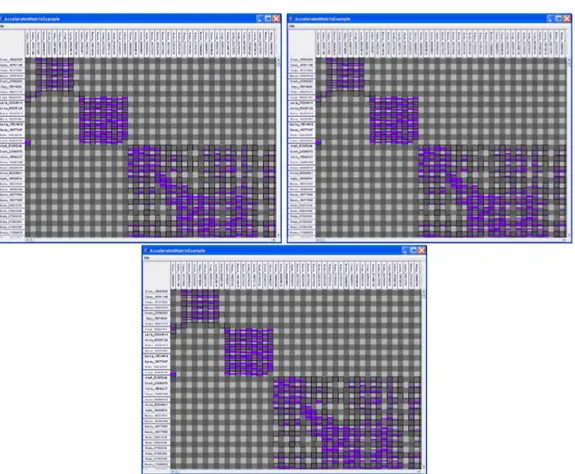
Figure 11: Graph visualization using the average (top), min/max (middle), and histogram (bottom) aggregate visual representations of the French Wikipedia dataset.

4, rue Jacques Monod - 91893 ORSAY Cedex (France)

Unité de recherche INRIA Lorraine : LORIA, Technopôle de Nancy-Brabois - Campus scientifique 615, rue du Jardin Botanique - BP 101 - 54602 Villers-lès-Nancy Cedex (France)

Unité de recherche INRIA Rennes : IRISA, Campus universitaire de Beaulieu - 35042 Rennes Cedex (France) Unité de recherche INRIA Rhône-Alpes : 655, avenue de l’Europe - 38334 Montbonnot Saint-Ismier (France) Unité de recherche INRIA Rocquencourt : Domaine de Voluceau - Rocquencourt - BP 105 - 78153 Le Chesnay Cedex (France)