HAL Id: hal-01055555
https://hal.inria.fr/hal-01055555
Submitted on 13 Aug 2014
HAL is a multi-disciplinary open access
archive for the deposit and dissemination of
sci-entific research documents, whether they are
pub-lished or not. The documents may come from
teaching and research institutions in France or
abroad, or from public or private research centers.
L’archive ouverte pluridisciplinaire HAL, est
destinée au dépôt et à la diffusion de documents
scientifiques de niveau recherche, publiés ou non,
émanant des établissements d’enseignement et de
recherche français ou étrangers, des laboratoires
publics ou privés.
A data type for discretized time representation in DEVS
Damian Vicino, Olivier Dalle, Gabriel Wainer
To cite this version:
Damian Vicino, Olivier Dalle, Gabriel Wainer. A data type for discretized time representation in
DEVS. SIMUTOOLS - 7th International Conference on Simulation Tools and Techniques, ICST, Mar
2014, Lisbon, Portugal. �hal-01055555�
A data type for discretized time representation in DEVS
Damián Vicino
Université Nice Sophia Antipolis, France Carleton University, Ottawa,
ON, Canada
Laboratoire I3S UMR CNRS 7271, France
[email protected]
Olivier Dalle
Université Nice Sophia Antipolis, France Laboratoire I3S UMR CNRS
7271
INRIA Sophia Antipolis -Mediterranée
France
[email protected]
Gabriel Wainer
Dept. of Systems and Computer Engineering Centre of Visualization and
Simulation (V-SIM) Carleton University, Ottawa,
ON, Canada
[email protected]
ABSTRACT
This paper addresses the problems related to data types used for time representation in DEVS, a formalism for the spec-ification and simulation of discrete-event systems. When evaluating a DEVS simulation model into an actual com-puter simulation program, a data type is required to hold the virtual time of the simulation and the time elapsed in the model of the simulated system. We review the commonly data types used, and discuss the problems that each of them induce. In the case of floating point we show how, under cer-tain conditions, the simulation can break causality relations, treat simultaneous events as non simultaneous or treat non simultaneous events as simultaneous. In the case of integers using fixed unit we list a number of problems arising when composing models operating at different timescales. In the case of structures that combine several fields, we show that, at the cost of a lower performance, most of the previous problems can be avoided, although not totally. Finally, we describe an alternative representation data type we devel-oped to cope with the data type problems.
Categories and Subject Descriptors
I.6.2 [SIMULATION AND MODELING]: Simulation Languages
Keywords
Simulation, Data Type, Time, DEVS
1.
INTRODUCTION
Discrete-event simulation is a technique in which the sim-ulation engine plays an history following a chronology of events. The technique is called ”discrete-event” because the processing of each event of the chronology takes place at discrete points of a time-line and takes no time with respect to virtual simulated time (even though it may take a non-negligible time to compute with respect to the real wall-clock
time). Unless the system being modeled already follows a discretized schedule (e. g. basic traffic lights), the process of modeling a phenomenon using a discrete-event simulator can be considered as a discretization process.
We will discuss some implementation issues related to the representation of the time in a discrete-event simulation en-gine. Since this problem is closely dependent on the im-plementation details, we choose to restrict our discussion to the particular case of the DEVS discrete-event simulation engines[2] [11]. The DEVS formalism provides a theoreti-cal framework to think about Modeling using a hierarchitheoreti-cal, modular approach.
The modeling hierarchy has two kinds of components: basic models and the coupled models. The basic models (with ports) are defined as a tuple:
A =< S, X, Y, δint, δext, λ, ta > where: S is the set of states,
X = {(p, v)|p ∈ IP orts, v ∈ Xp} is the set of input ports and values,
Y = {(p, v)|p ∈ OP orts, v ∈ Yp} is the set of output ports and values,
δint: S → S is the internal transition function, δext: Q × X → S is the external transition function, Q = {(s, e)|s ∈ S, 0 ≤ e ≤ ta(s)} is the total state set (with e is the time elapsed since last transition), λ : S → Y is the output function and
ta : S → R+
0,∞ is the time advance function.
At any time of the simulation the basic model is in a specific state awaiting to complete the lifespan delay returned by the ta function, unless an input of a new external event occurs. If no external event is received during the lifespan delay, the output function λ is called, and the state is changed accord-ing to the value returned by the δintfunction. If an external event is received, then the state is changed to the value re-turned by the δextfunction, but no output is generated. Coupled models define a network structure in which nodes are any DEVS models (coupled or basic) and links represent the routing of events between outputs and inputs or to/from upper level. Formally, the Coupled Models are also repre-sented by a tuple:
C =< X, Y, D, M, EIC, EOC, IC, SELECT > where: X is the set of input events,
Y is the set of output events,
D is an index for the components of the coupled model, M = {Md|d ∈ D} is a tuple of basic models as previously defined,
EIC, EOC, and IC are respectively the External Input Coupling, External Output Couplings and Internal Cou-plings that explicit the connections and port associations respectively from external inputs to internal inputs, from internal outputs to external outputs, and from internal out-puts to internal inout-puts,
SELECT : 2D− {} → D is the tie-breaker function that sets priority in case of simultaneous events.
Zeigler[11] also described the algorithm of a simple abstract simulator, able to execute the DEVS models. When it exe-cutes a model, this simulation algorithm exchanges only two types of data with the models: events and time.
In the last four decades, many DEVS simulation engines have been implemented and studied using different com-putation models, such as Sequential, Parallel, Distributed, Cloud, etc. All these DEVS engines handle the passing of events between models following the principles of the ab-stract simulator: Compute the time of next events (mini-mum of the times remaining in each model until the next internal transition), compute resulting event outputs, route events in the network to their destination inputs, and recom-pute the time remaining until the next round (subtracting the time elapsed from the scheduled time advance). Notice that time is never exchanged directly between mod-els, but only between the models and the simulation engine. Therefore, a common time representation is needed between the models and the simulation algorithm, but this time rep-resentation can possibly vary from one model to another, provided that the simulation algorithm is able to make the translation.
Simultaneous events correspond to the cases in which the discretization that results from the discrete-event modeling produces identical time values. Simultaneous events occur in DEVS in two ways: either a model receives input events from multiple models at the same time, or it receives events from other models at the same time as it is reaching the end of the time advance delay. Some means are provided in each DEVS variants to ensure deterministic processing of simultaneous events. For example, in classic DEVS, a tie-breaker function named SELECT is used to resolve this situation.
The SELECT function is hard to define, and having an er-ror in its definition can lead to unpredictably large modeling errors, as will be discussed in Section 3. However, assuming the SELECT function used is valid, we may still experi-ence simulation errors due to the way the time is stored internally by the simulation engine. Indeed, in the DEVS formalism, the time is a real value, but it is well known that it is not possible to find a computer representation for all real numbers. Therefore, an approximation is needed for the values that have no exact representation. This approxima-tion is the result of a quantizaapproxima-tion process. Unfortunately, contrary to modeling errors, simulation errors due to the quantization of time are hidden to the modeler even though
they may have similar impact on the simulation results. The focus of this paper is on this particular problem of se-lecting an internal representation and the possible effects of such a selection on the simulation results.
2.
BACKGROUND
To contextualize the problem, we reviewed the source code and documentation of the eight following DEVS simulator projects:
• ADEVS[9]: “A Discrete EVent System simulator” is developed at ORNL in C++ since 2001;
• CD++[8]: “Cell-DEVS++” is developed at Carleton University, in C++, since 1998;
• DEVSJava[12]: “DEVJava” is developed at ACIMS in Java since 1997; it is based on its predecessor DEVS++[6] (implemented in C++). Currently it is part of the DEVS-Suite project[10];
• Galatea: A bigger project with an internal component (Glider) developed at Universidad de Los Andes im-plementing DEVS in Java since 2000;
• James II[5]: “JAva-based Multipurpose Environment for Simulation” is developed at University of R¨ostock, in Java, since 2003. It is the successor of the simulation system JAMES (Java-based Agent Modeling Environ-ment for Simulation). The project includes a set of Simulators, we reviewed the DEVS one;
• ODEVSPP[6]: “Open DEVS in C++” is developed in C++, since 2007;
• PyDEVS[1]: “DEVS for Python” is developed at Mc Gill University in Python since 2002;
• SmallDEVS[7]: “SmallDEVS”is developed at Brno Uni-versity of Technology in SELF/SmallTalk since 2003. A common feature in all of them is to embed the passive state representation in the time representation data type using some infinity representation.
All simulators, but ADEVS and CD++, represent Time us-ing the double precision floatus-ing point data type1
provided by the programming language. All but one use the internal representation of infinity provided by the data type. The exception is ODEVSPP that uses MAX DOUBLE constant in place of internal infinity.
In the case of ADEVS the time is represented using a C++ class template. The class works as a type wrapper adding infinity representation to the provided type. The operators are defined in a way that, if one of the parameters is an infinity the defined algorithms are used, else the wrapped type operators are used.
In the case of CD++ the time is represented using a class with five attributes: four integers for the hours, minutes, seconds and milliseconds, and a double precision floating point for sub-milliseconds timings. There is not an explicit representation of infinity, but the passive state is evaluated comparing the Hour field to 32767.
1
In the case of PyDEVS, the dynamic type is forced to Float-ing Point by systematically usFloat-ing Python castFloat-ing syntax.
Something to keep in mind is that all DEVS simulators exe-cute a single Model (sometimes composed of several others). This model is called the top or root model.Regardless of the simulator, a global variable is needed to keep track of the global Simulation Time. Some simulator may try to reduce the scope of the synchronization in sub-models wherever it is possible, while others simply use the root model in a sys-tematic way to centralize all timing information. This is important to remember when evaluating Time representa-tion range.
3.
TIME REPRESENTATION PROBLEMS
In DEVS modeling, the domain of the time variables is R+. This choice results in a quantization problem at the time of implementing the model. Depending on the data type chosen for implementation, different approximations or re-strictions may be observed.
Approximation effects belong to two categories: time shift-ing, and event reordering. In the case of time shiftshift-ing, we have an error on the precision of the computation, but the time line of events is not affected. In the second case, the approximation leads to a different time line of events than the one expected in theory using exact arithmetic on real numbers, which may, in turn, break the causality chain. In case the causality chain is broken, the error can be arbi-trarily large, such that no error bound can be found in the general case.
A characteristic of reordering errors is that they cannot be explicit in formal proofs on the paper. Furthermore, reorder-ing errors are practically impossible to predict, and may occur following irregular frequency patterns, which, in the worst case, can fool the validation tests.
The following example shows that even the simplest model may be subject to reordering errors. In this example, we model a counter with 2 inputs, one to increase the count and the other to reset and output the current counter result. The root coupled model is:
C =< X, Y, D, M, I, Z, SELECT > where: X = ∅,
Y ⊆ {out} × N,
D = {1, 2, 3} with: M1 and M2 two generators sending tick respectively every 0.1 second and every 1 second, and M3a counter with 2 input ports: add 1 and reset.
EIC = ∅, EOC = {((M3, out), (self, out))},
IC = {((M1, out), (M3, add1)), ((M2, out), (M3, reset))} SELECT defined to give priority to inputs from model M1 over those from model M2.
The output of this simulation is, in theory, the value 10 on the ”out” port of C every 1 second.
We implemented this in DEVSJAVA 3.1 and pyDEVS 1.1, and kept it running for a while. In DEVSJava we got a differ-ent result than expected: the output consisted of a majority of 10 values, but also some 9 and 11 values. In pyDEVS we first obtained the expected results for this experiment. Nevertheless, after changing the parameter of M2 from 1.0 to 100.0 seconds, we observed similar discrepancies, with a few occurrences of 999 and 1001 values on C’s “out” port
instead of only 1000 as theoretically expected. Interestingly, the errors of this model occur following a regular pattern (a geometric law of factor 4 in both simulators).
This result can be explained knowing that both simulators use single or double precision Floating Point numbers for time representation. Indeed, the value 0.1 is well-known bad quantization point in the Floating Point standard. There-fore, every time an algorithm accumulates many times the value 0.1, as the model M1 does, the rounding error accu-mulates, which leads to the observed errors. We discuss in more details the case of Floating Point numbers in section 3.1.
Looking at other data types, such as Integers for example, does not fully solve the problem. We further discuss the case of integers in section 3.2.
In Section 2, we also reviewed implementations that use a structured or object-oriented data-type. However, as further explained in section 3.3, these data-type don’t have bet-ter results than using floats or integers because they work mostly as wrappers of these types or small extensions to their range.
3.1
Floating point data types
Adopted by a majority of simulators, this data type leads to several variants due to the selection of different preci-sion levels (single, double, or extended) and how the passive state of a model is represented (the semantics of which be-ing to wait for an infinite time). For example, infinity can be mapped onto a reserved value or an additional variable, e. g. a boolean, can be use to handle the special case of infinity, in a structure or wrapper data type.
3.1.1
Strengths of floating point
The floating point data type was engineered to represent an approximated real number and to support a wide range of values. The basic structure is the use of a fixed length mantissa and a fixed length exponent.
The main strengths of using floating points are:
• A compact representation, usually between 32 and 128 bits;
• Implemented in almost every processor;
• A large spectrum between max and min representable numbers;
• An internal representation for infinities;
• A widely used standard, making the simulator code more portable;
• Largely studied mechanics of its arithmetic approxi-mations.
On the other hand, floating point has well known limita-tions[4], but are still often considered as an acceptable trade-off, due to their intuitive use. We review those problems and limitations in the following sections, in the particular case of simulation. It is important for the analysis to notice that the only operations used internally by the DEVS Simulator on time values are additions, subtractions and comparisons.
The floating point arithmetic rounds the results continu-ously, not only with divisions (as it happen with integer), but also with additions and subtractions. Rounding errors result in two kind of errors: shifted values, and artificially coincidental values.
We don’t elaborate more on the case of shifted values, as this case was already discussed with the example in the previous section, that showed this kind of error can easily break the causality chain, e. g.. by accumulation.
The rounding of values due to quantization may also pro-duce artificially coincidental values. As mentioned in the introduction, the case of simultaneous events must be dealt with care, which explains the need for a SELECT func-tion. Unfortunately, when the coincidence is the result of a hidden process, the SELECT function may not be able to make a proper decision. Indeed without the rounding er-ror, two distinct time values have an implicit natural order, and this natural order may not be the one produced by the SELECT function.
3.1.3
Non fixed step
The floating point representation uses a variable step size be-tween consecutive represented values. The reasons for hav-ing variable step come from the nature of the incremental sequence of powers: As the absolute value of the exponent value increases, more bits are needed for coding the expo-nent value, and these bit are taken from the least significant side of the mantissa.
Some assertion code can be provided to detect when an ad-dition of non zero numbers is done and to check if the result is equal to one of the operands.
3.1.4
Cancellation
This kind of problem happens when subtracting 2 close num-bers. The effect is that the mantissa loses precision. For instance, when subtracting 0.999 from 1.000, we get 0.001: The mantissa digits are shifted to obtain 1.0E-3, and the result is the loss of the 3 significant digits in the mantissa. This cancellation effect makes the rounding problem even worse.
A solution sometimes proposed to solve some of the float-ing point issues, since the time always advances, is to use a framing mechanism. This is a way to keep the computa-tions in the dense area around the origin. This solution is implemented using a threshold value t0: Once the models have reached this value, t0 is subtracted from all the clocks in the system.
A downside of this solution is that it increases the number of subtractions, which in turn may lead to an increase in Cancellation errors.
Error detection can be implemented by keeping track in ev-ery operation of how the mantissa significance was affected. This does not solve the problem, but may still give a confi-dence indicator as the assertion in the non fixed step one.
3.1.5
Compiler optimization dangers
In 1991 Goldberg[4] shows a set of optimizations that when used with floating points can affect the precision of the com-putation. Changing compilers (for updating or portabil-ity) can change results if any problematic optimization is added or removed, which might be hard or impossible to detect.Also, at the time of distributing the simulation in an heterogeneous cloud or grid, different architectures, operat-ing systems and compilers may be used makoperat-ing the problems scale together with the infrastructure.
3.1.6
Standard complexity
If the floating implementation follows the IEEE754, which is common, there are more issues to consider. IEEE754 gives special meaning to some quantities (NAN, Infinities, pos-itive and negative zeros); it defines exceptions, flags, trap handlers and the option to choose a rounding models. These mechanisms need to be taken into account when implement-ing the Simulator, or they could result in unexpected behav-iors.
3.2
Integer data types
Using integers is the first idea that comes up when trying to avoid the issues related to rounding and precision with float-ing point numbers. For example, in the field of networkfloat-ing, well-known simulators such as NS and Omnet++ have gone through major rewriting in order to change their represen-tation from floating point to integers: NS3 has chosen a 128 bits integer representation, while Omnet++ v4.x has chosen a 64 bits integer representation.
3.2.1
Strengths of integers
The Integer type is used to represent a subset of consecutive numbers in Z.
Some interesting characteristics of the Integer type are: • Its compact representation, usually between 8 and 128
bits;
• Its generalized support by all processors;
• Its fast and exact arithmetic, except for divisions; • Its fixed step between any two consecutive values; Using integers in place of floats can be seen as a trade-off in which the large range and the ability to approximate the (dense) real numbers is traded against the accuracy of an exact representation, but only for a limited range of the (sparse) natural numbers. In many situations, when the range is not that much a concern, integers offer a better trade-off.
3.2.2
Overall range
For a given number of bits, the absolute range of values supported by an integer type using that amount of bits is much narrower than the absolute range of a floating point using the same amount of bits. Indeed, starting with the single precision floating point (32 bits), the largest absolute value is around 3 × 1038
while it is only around 2 × 10⁹ for a 32 bits integer; At the other end, the smallest single precision floating point value is around 1 × 10−38
while for any positive integer the smallest (absolute) value is 1. Trying to cover the same range as a floating point with
in-tegers, using the smallest step offered by the floating points, is feasible but very space-inefficient for single precision (76 bits vs. 32) and unreasonable for higher precision.
However, since there is no approximation with the additive arithmetic on integers, a frame shifting mechanism as de-scribed in previous section is safe to implement and will not incur problems such the cancellation mentioned about float-ing points.
3.2.3
Quantity of unused representation
Since the smaller representable value is 1, the unit associated to the variable is the smallest representable time of a model. Some simulator use a fixed unit value, e. g. nano-seconds. This fixed unit implies that all timings are aligned on mul-tiples of one nanosecond. Therefore, a model of a generator that would output ticks every second, would waste 99.9% of an already limited representation range.
To avoid this waste, an analysis of the model can help to adjust the unit. In this case, the unit does not need to be a standard one: a rational, eg. 1
7s, can even be chosen if it allows to capture all the possible timings needed for the simulation of the model time line.
3.2.4
Multiple scales and model composition
One of the strengths of the DEVS formalism is its ability to compose models. This favors the reuse of previously devel-oped models to create more complex ones and the division of the system into smaller parts.
Assuming the time unit is hard-coded within the Simulator implementation requires a unit to be found that covers all possible models. This approach can be used for simulators dedicated to a specific purpose, eg. micro-controllers elec-tronics or planets dynamics. However, if the simulator is intended to be multi-purpose, it becomes impossible to find a compact and efficient representation that covers the full spectrum of possible requirements.
An alternative is to use time units defined locally within each model. For instance, this approach allows to pick months as the time unit for building a gravitational model of plan-ets dynamics, and pico-seconds for micro-controllers as sug-gested by each model analysis.
When we have different time scales in different (Sub-)models, we need to have extra computation to compose them as DEVS Coupled Models. In case the time-step in one repre-sentation is divisible by the one in the other, the smallest step can be used as the common step, but the time-values in the larger-step model have to be systematically adjusted, at the cost of an extra multiplication operation.
When using time-scales that don’t divide each other, e. g. 1
7s and 1
5s, finding a common time-step requires to find a common denominator, and adds a systematic multiplication on both sides.
3.3
Structures and containers
Complex data types that come with each programming lan-guage can also be used be used in place of the afore-mentioned
ones, in order to avoid some of the problems we have sur-veyed. These data types include: classes, objects, structs, tuples, arrays, vectors and other containers.
However, using such data types often results in new trade-offs, such as user-friendliness vs. memory consumption, or vs. performance, or vs. complexity of time arithmetic.
3.3.1
Developer friendliness
In some implementations of time, a structure with an integer fields to handle different units of a time value is used. This can be done using an array, vector, class or struct, with the main objective of expanding the range.
This kind of structure is used in the Time class in CD++ (which has also an extra float field) in which the fields are aligned on standard time sub-units (days, hours, minutes, nanoseconds). The use of human-friendly units, even when convenient for the model definition, makes the arithmetic more complicated, and is space inefficient. For example, using a byte-long integer to represent minutes on 8 bits, wastes 76% of the values.
3.3.2
Memory consumption and access
Integers and floating point numbers can both use either 16, 32, 64 or 128 bits depending on the processor architecture. A struct having multiple integers as previously defined, when implemented as a Class, Object or Struct, requires a pointer to the structure and offsets to each component.
This gets worst if we combine with previous problem and we use human friendly representation. For efficiency purpose, it is advisable to use integer that match the processor register size, hence at least 64 bits on computing architectures cur-rently available. An structure for [HH:MM:SS] using such integers for each field would use 224 bits and represent less range than a single 64 bits integer coding the same range using the seconds unit. In some languages, like C++, this can be reduced choosing an 8 bit integer data type, anyway this is not a possibility in some other languages like PHP or Python.
In case a vector-type collection is used, the memory footprint is increased to define pointers needed for iteration or other general purpose use of the data type as memory allocators. In some architectures with few available registers, accessing multiple integers generates a higher number of cache miss and results in significant performance degradation.
3.3.3
Memory Alignment
In most architectures, the use of smaller than bus size or misaligned data types will require extra processing to be read and write. For example, if the bus width is 32 bits, 2 consecutive integer values of 16 bits can be read using a single memory access, but extra operations are needed for the actual values to be unpacked prior operation. Similarly, having a 16 bits integer followed by a 32 bits one ends up either with the second one being misaligned and requiring two memory access each time it is read/write, or with the waste of 16 bits to realign the representation.
3.3.4
Operation encapsulation
If we want this data type to be reusable, the operations giv-ing the semantic to the data type and its representation need to be encapsulated. The only data types providing the mech-anisms to embed operations in a data type are classes and objects, and in most languages one depends on the other. This encapsulation has to be compared with the usability of collections. In case the data type is first designed as a class or object, adding the operators to it doesn’t increase the memory access to its internal fields. On contrary, in case the data-type is designed as the encapsulation of a collection, using a class or object wrapper, a new indirection level is added, which may result in increasing the number of memory access, with possible added degradation due to cache miss.
4.
A NEW TIME DATA TYPE
The standard way to represent the measure of a time lapse is the product between its magnitude and the time unit: t = m × u. Our proposed data-type aims as finding how to best represent both of these quantities, the magnitude and the unit.
In Section 3 we described a set of problems and limita-tion with the representalimita-tion and performance of the differ-ent data types used in DEVS implemdiffer-entations. Looking for a more adequate data type for the time computation in DEVS, we describe in the following subsections a set of rep-resentation requirements, performance requirements and we propose a data type covering most of those requirements to avoid the previously exposed problems.
4.1
Representation requirements
From previous analysis, we can derive the following require-ments:
• For the unit part of the representation, different units must be supported;
• For the magnitude part, we need to address four con-cerns:
1. Avoid (hidden) quantization as much as possible; 2. Avoid additive arithmetic errors;
3. Provide a large enough range for any time repre-sentation;
4. Support seamlessly the coupling of models possi-bly operating using different units;
• Optionally, we may want to have an internal represen-tation for infinity. (Some simulators don’t need it.)
4.2
Performance requirements
We expect the use of the new data type not to impact signifi-cantly the performances of the simulation. Time is advanced in every model, and every coordinator has to operate with it.
We should keep our representation compact and avoid wast-ing representation space.
Also, when trade-offs for performance are possible, we prefer to optimize the additive operations and comaparisons, which are the only ones used internally by the simulator.
Since time scaling operations that result from the composi-tiopn of models may be expensive, we want to avoid them as much as possible.
4.3
The proposed data type
In this subsection, we first describe a data type that cov-ers the representation requirements and enumerate it limita-tions. Afterward, we describe how to, doing a few trade-offs, we can adapt it to a more performant implementation. For the magnitude, we need a representation that allows us to represent large subset of numbers without rounding, and that all operations result in values into the same subset. A large subset of R covering this 2 conditions is Q, any of its values q can be represented as q = qn
qd where qn, qd∈ Z. A representation of numbers in Q includes the numbers of the Integer type representation and the numbers of the Floating Point type representation (but infinity). In ad-dition, it covers new cases, such as the numbers required for representing frequencies that are not powers of 2. I.e. two generators, one sending three events per second and one sending one per second can be modeled and have a si-multaneous event every second.
Unfortunately, a simple implementation of this data type re-quires more space and operations time than previous ones. The space complexity comes from having several pairs of integers that represent the same value. The time complex-ity comes from the need to compute reductions (Greatest Common Divisor) in the representation in order to keep it as compact as possible.
Recall from earlier that we note t = m × u.
To ensure that the range, m, can be large enough, a dy-namic size representation can be used for the numerator and denominator. In the following, we assume m is a ra-tional number q defined by a duple of integers that are large enough.
For u, the unit, we can use an enumeration of units and define the scaling function to convert the operands of binary arithmetics operations to the smallest common unit before proceeding.
The previous data types covers all the representation re-quirements.
The restriction is that magnitude values had to be sented by a subset of Q delimited by the size used to repre-sent the 2 integers used to reprerepre-sent q and the units need to be a finite predefined set with relations well defined between them.
Unfortunately, using this data in a real simulation would waste a lot of representation space, and induce a big com-putation overhead when coupling models havoing different units.
A few optimization can help reduce this overhead in the general case and limit the increase of complexity to specific scenarios that where not supported by previous data types.
A first change is to replace the unit enumeration represen-tation by an integer scale factor e and a patron unit p, so that any unit can be thought as p × 2e. Using the Second as patron unit may be reasonable for general purpose if the e is represented with a 32 bit integer.
The second change would be to use a custom quantum qu ∈ Qand a scale i ∈ Z to represent the time inside each model as: qu×i. This quantum is a divisor of all the possible times that will be used by the model, modelers usually think about it at the time of modeling. In the case the modeler doesn’t set the quantum, if the model has regularity in its behav-ior, qu can be readjusted by the Simulator automatically (by finding the Greatest Common Divisor between last used qu and the one from current operation), until a stable state is reached. An example of a case where it never reaches stability is when the frequency of events is continuously in-creasing, eg. with ta = (1
2)
n where n is the quantity of previous outputs.
Thanks to this quantum, all operations that apply to operands having the same quantum, which is expected to be a most common case, become Integer computations. In case operands have different quantum, a quantum adjustment is needed, which may be an expensive operation used few times. The case in which an adjustment is needed very frequently corre-sponds to a model that was not properly handled by previous representations.
We propose then to reduce the qu representation to two com-mon integers as large as the architecture bus. This trade-off of keeping a small qu can increase significantly the optimiza-tion possibilities of the data type and keep it compact. This reduction is not as restrictive as it may look, when combin-ing to the unit representation all float and integer space is covered and we still have another component i to scale the values.
If we look the whole representation (magnitude and unit), with current changes a time lapse is represented as: t = i × qu × 2e
× p. In 32 bits architecture, the qu takes 64 bits, the e 32 bits, p is implicit and i we can fix it to 32 bits too and have a representation of 128 bits which most the time the operations are just comparison of the first fields and add/substract/compare on the last one, all possible with 32 bits Integer operations.
To simplify the notation, we define the unit u as: u = qu × 2e
× p and the time lapse t as: t = i × u.
When working with binary operators, if both operands have the same unit, the computation only involves i part of each operand. The problem of having the i part limited to 32 bits is the coupling of models using different units, which makes necessary to have binary operators supporting different units in their operands. If the two unit differ in scale (different value of e), the computation applies only to the overlapping segments of the qu part, but we need to check for possible carry to expand the representation.
In case the quantums of each time value are different, a com-mon quantum needs to be found and then i and e adjusted accordingly. Since this is a more expensive operation, a
good selection by the modeler of the quantum of each model is important to quickly reach a stable state with a common quantum.
A way to agree on the value of qu can be added either to the Simulator logic so the models negotiate it at initialization, or it can be encapsulated in the Time data type itself if using an Object Orient Language.
The problem with the initial negotiation approach is that it extends the logic of the simulator and doesn’t really solve the problem when the time unit can change during simulation (as the model ticking half as previous tick showed before). Anyway, if the trade-off is worth it between predictability on the performance and flexibility to allow the change of the quantum in simulation time, it can be done.
In the dynamic case, a simple implementation of the nego-tiation mechanism that agrees in a global qu common to all models participating can be implemented just checking
qulocal = quglobal at the time of operate, if they are equal
then just operate with no worry, in the case they are not equal a new qugloabl that divides both is computed, the lo-cal i and e are adjusted and the new qu is assigned to both. All models defined with different qlocal will do this until reach consensus. Obtaining consensus using this approach is lineal in the quantity of basic models participating in the simulation, anyway stabilization of the representation in ev-ery model can require square of the quantity of Basic Mod-els adjustments to internal representation variables. This approach after reach consensus is as performant as the pre-vious one, but it doesn’t exclude the use of Models that can change its qu. If a model changes it qu a new consensus needs to be reached, and automatically will be done. The header of a Time c++ class with a mechanism to agree the q encapsulated may look like this:
t y p e d e f pair <int, int> f r a c t i o n ;
t e m p l a t e <t y p e n a m e T > class Time { p u b l i c: // c o n s t r u c t o r s Time () = d e l e t e; Time (const f r a c t i o n q ,
const int exp ,
const int m ) ;
// o p e r a t o r s
Time & o p e r a t o r=(const Time &) ;
const Time o p e r a t o r+(const Time &) ;
Time & o p e r a t o r+=(const Time &) ; // n e g o t i a t i o n s t a t i c f r a c t i o n q _ g l o b a l ; p r i v a t e: f r a c t i o n q _ l o c a l ; B i g I n t i ; int e ; }; // C o m p a r i s o n o p e r a t o r s
bool o p e r a t o r==(const Time & , const Time &) ;
bool o p e r a t o r!=(const Time & , const Time &) ;
bool operator<(const Time & , const Time &) ;
bool operator>(const Time & , const Time &) ;
bool operator<=(const Time & , const Time &) ;
This c++ class implementing the operations as described earlier in this section covers fairly the requirements. Another representation can be done changing the i and e data types to vector of pair of integers where each position in the vector has a segment of i and an associated e. This way, when operating between numbers that don’t have dig-its in common, the addition or subtraction can be done as just a concatenation. Also, this representation saves space when several 0s are in the middle after an operation, this are just not represented in the vector, any segment of 0s can be removed from the vector.
About complexity of the operations in the alternative repre-sentation. For add/subtract operations once the qu is stable the operations need to do a check of the compatibility and then the operation as described before. If we simulating something that was possible to simulate using Integers, the overhead is 3 integer compares for equality, if it was not pos-sible to simulate the worst case is linear to the size of the vector used to represent i. If the vectors don’t have gaps and the e matches, complexity is equivalent to use BigInt, in the case there is any gap or the e is miss-aligned a displacement of all segments may be done in the worst case and this is a linear operation in the size of the i vector. For the compare operations worst case is linear to the size of the i vector too.
4.4
Communicating values
From previous analysis, we can think about how to com-municate models in different simulator modules to handle interaction with web server based simulator or between dif-ferent technologies.
An XML, JSON, or any serialization can be provided based in the class header described before.
An message using xml, may look like this: <?xml v e r s i o n=" 1.0 "? >
< time type =" Time "> < unit n u m e r a t o r =" 58 " d e n o m i n a t o r =" 57 " patron =" Second " / > < m a g n i t u d e offset =" -64 "> 1 2 3 8 1 2 9 3 7 1 2 9 8 3 7 1 2 9 </ m a g n i t u d e > </ time >
The magnitude can be broke in pieces and send the offsets and content of the segments and avoid completing the gaps with 0s. Anyway, given the time it takes to parse the XML the difference may not be significant and more validation is needed to check the overlaps when parsing.
5.
PERFORMANCE COMPARISON
In this section, we show the results of 4 experiments we realized to measure the performance impact of choosing the proposed Data Type compared against other possible Time data types implementation.
The experiments are implemented in C++11 compiled with clang 500.2.79. Each experiment was run without compiler
optimization and with -O2 compiler optimization. Five data types are used for comparison:
• Float: We use the native float implementation. • Integer: We use the native integer wrapped in a class
to make it also provide infinity arithmetic.
• Rational : We use the boost[3] implementation of ra-tional (1.55) wrapped in the same class as Integer to make it also provide infinity arithmetic.
• DTime: A naive implementation of the proposed data type using global agreement with statics as described in previous section.
• FDTime: A naive alternative implementation to the proposed one. This one doesn’t intent to reach global agreement, in place the agreement is produced between operands in each operation.
5.1
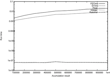
Experiment: series y=1
This experiment implements: PN
x=11 0.0001 0.001 0.01 0.1 1 100000 200000 300000 400000 500000 600000 700000 800000 900000 1e+06 Run time Acumulation result FDTime DTime Float Integer Rational
Figure 1: Seriesy = 1 with no compiler optimization.
1e-08 1e-07 1e-06 1e-05 0.0001 0.001 0.01 0.1 100000 200000 300000 400000 500000 600000 700000 800000 900000 1e+06 Run time Acumulation result FDTime DTime Float Integer Rational
Figure 2: Series y = 1 with -O2 compiler optimiza-tion.
In this experiment all types but float provide exact results. The problem with float is that after accumulating enough,
the exponent is increased and the increment starts being discarded.
In Fig. 1 all data types show similar behavior, the worst implementation appears to be the Rational, while both FD-Time and FD-Time appear to be similar to just using an Integer with Infinity operations.
In Fig. 2 Integer and Rational are as good as float after being optimized, while FDTime and DTime get almost no improve from the compiler optimization.
5.2
Experiment: series y=1/x
This experiment implements: PN x=1
1 x
Computing this series using integers makes no sense and computing it using float is very imprecise, it rounds most of the values. 1e-07 1e-06 1e-05 0.0001 0.001 0.01 0.1 0 2000 4000 6000 8000 10000 12000 Run time N FDTime DTime Float Rational
Figure 3: Seriesy = 1/x with no compiler optimiza-tion. 1e-08 1e-07 1e-06 1e-05 0.0001 0.001 0.01 0.1 0 2000 4000 6000 8000 10000 12000 Run time N FDTime DTime Float Rational
Figure 4: Seriesy = 1/x with -O2 compiler optimiza-tion.
In Fig. 3 we obtain very similar results in DTime, FDTime and Rational and a float that goes 100x times faster (but returns the wrong results).
In Fig. 4 after run compiler optimizations, we see that float flattens getting a great improve, but the other data types are mostly unaffected by the optimizations, just doing slightly better at the start.
5.3
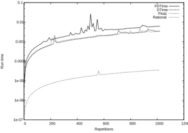
Experiment: series 1/
2x This experiment implements: PNx=1P23y=1 1 2y
This experiment returns all representable values in float un-til the exponent is increased. In numeric methods, it may be suggested to start the Sum from the smaller number to reduce the error. Anyway, in DEVS, we don’t have a way to reorder the operations, so it is a valid use case doing it this way. 1e-07 1e-06 1e-05 0.0001 0.001 0.01 0.1 0 200 400 600 800 1000 1200 Run time Repetitions FDTime DTime Float Rational
Figure 5: Seriesy = 1/2xwith no compiler optimiza-tion. 1e-07 1e-06 1e-05 0.0001 0.001 0.01 0.1 0 200 400 600 800 1000 1200 Run time Repetitions FDTime DTime Float Rational Figure 6: Series y = 1/2x
with -O2 compiler opti-mization.
In Fig. 5 we obtain similar results to previous experiment. In Fig. 6 something changes, this time the float curse doesn’t flatten.
5.4
Experiment: series 1/p
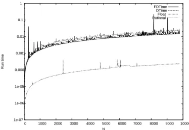
This experiment implements: PNx=1 1
pi with pithe i-esieme
Here, all numbers but 1/2 are not representable by float, so the result is very imprecise, also the prime numbers force to fail the simplification of the fractions in the internal repre-sentation of the other data types.
1e-07 1e-06 1e-05 0.0001 0.001 0.01 0.1 1 0 1000 2000 3000 4000 5000 6000 7000 8000 9000 10000 Run time N FDTime DTime Float Rational
Figure 7: Series y = 1/pi where pi is the i-esieme prime with no compiler optimization.
1e-08 1e-07 1e-06 1e-05 0.0001 0.001 0.01 0.1 0 1000 2000 3000 4000 5000 6000 7000 8000 9000 10000 Run time N FDTime DTime Float Rational
Figure 8: Series y = 1/pi where pi is the i-esieme prime with -O2 compiler optimization.
In both, Fig. 7 and 8, we obtain similar result to those in thePNx=11
x experiment.
6.
CONCLUSIONS
We surveyed a set of Simulators used to run DEVS formal-ism simulations and we analyzed the implications of the data type selected in those to characterize the need of a new Time data type. From this characterization we described require-ments for the new data type and a possible implementation which covers them at the expense of a slight increase in spa-cial and time complexity compared to its predecessors when running in the same scenarios, but increases significantly the accuracy and the range of the data type compared to previous ones. We compared naive implementations of the proposed Data Type against other Data Types used in the surveyed simulators and against other data types, the worst
penalty obtained was in the order of 100X. We think the trade-off is worth it even when work need to be done in op-timizing and compacting the data type yet. We will focus our future work in the complexity aspects, the implementa-tion and evaluaimplementa-tion of the data type in the CD++ simulator and then we will study how this work applies to other Sim-ulation formalisms in discrete events.
7.
REFERENCES
[1] J.-S. Bolduc and H. Vangheluwe. A modeling and simulation package for classic hierarchical DEVS.
MSDL, School of Computer McGill University, Tech. Rep, 2002.
[2] A. Chow and B. P. Zeigler. Revised DEVS: a parallel, hierarchical, modular modeling formalism. In
Proceedings of the SCS Winter Simulation Conference,
1994.
[3] R. Demming and D. J. Duffy. Introduction to the
Boost C++ Libraries; Volume I-Foundations. Datasim
Education BV, 2010.
[4] D. Goldberg. What every computer scientist should know about floating-point arithmetic. ACM
Computing Surveys (CSUR), 23(1):5–48, 1991.
[5] J. Himmelspach and A. M. Uhrmacher. Plug’n simulate. In Simulation Symposium, 2007. ANSS’07.
40th Annual, pages 137–143. IEEE, 2007.
[6] M. H. Hwang. DEVS++: C++ Open Source Library
of DEVS Formalism. On-line resource at
http://odevspp.sourceforge.net/ [Last checked: Oct 31st 2013], v.1.4.2 edition, April 2009.
[7] V. Janouˇsek and E. Kironsk`y. Exploratory modeling with smalldevs. Proc. of ESM 2006, pages 122–126, 2006.
[8] A. L`opez and G. A. Wainer. Improved Cell-DEVS model definition in CD++. In Proceedings of ACRI.
Lecture Notes in Computer Science, volume 3305,
Amsterdam, Netherlands, 2004. Sloot, P.; Chopard, B.; Hoekstra, A. Eds.
[9] J. Nutaro. ADEVS project. On-line resource at http://web.ornl.gov/˜1qn/adevs/ [Last checked: Oct 31st 2013].
[10] X. Xiaolin Hu and B. P. Zeigler. The Architecture of
GenDevs: Distributed Simulation in DEVSJAVA.
On-line manual at http://acims.asu.edu/wp- content/uploads/2012/02/The-Architecture-of-GenDevs-Distributed-Simulation-in-DEVSJAVA-.pdf [Last checked: Nov 1st 2013], January 2008.
[11] B. P. Zeigler, H. Praehofer, T. G. Kim, et al. Theory
of modeling and simulation, volume 19. John Wiley
New York, 1976.
[12] B. P. Zeigler and H. Sarjoughian. Introduction to DEVS modeling & simulation with JAVATM: Developing component-based simulation models.