HAL Id: hal-00318351
https://hal.archives-ouvertes.fr/hal-00318351
Submitted on 30 Jul 2007
HAL is a multi-disciplinary open access
archive for the deposit and dissemination of
sci-entific research documents, whether they are
pub-lished or not. The documents may come from
teaching and research institutions in France or
abroad, or from public or private research centers.
L’archive ouverte pluridisciplinaire HAL, est
destinée au dépôt et à la diffusion de documents
scientifiques de niveau recherche, publiés ou non,
émanant des établissements d’enseignement et de
recherche français ou étrangers, des laboratoires
publics ou privés.
Low latitude ionosphere-thermosphere dynamics studies
with inosonde chain in Southeast Asia
T. Maruyama, M. Kawamura, S. Saito, K. Nozaki, H. Kato, N. Hemmakorn,
T. Boonchuk, T. Komolmis, C. Ha Duyen
To cite this version:
T. Maruyama, M. Kawamura, S. Saito, K. Nozaki, H. Kato, et al..
Low latitude
ionosphere-thermosphere dynamics studies with inosonde chain in Southeast Asia. Annales Geophysicae,
Eu-ropean Geosciences Union, 2007, 25 (7), pp.1569-1577. �hal-00318351�
www.ann-geophys.net/25/1569/2007/ © European Geosciences Union 2007
Annales
Geophysicae
Low latitude ionosphere-thermosphere dynamics studies with
inosonde chain in Southeast Asia
T. Maruyama1, M. Kawamura1, S. Saito1, K. Nozaki1, H. Kato1, N. Hemmakorn2, T. Boonchuk2, T. Komolmis3, and C. Ha Duyen4
1National Institute of Information and Communications Technology, 2-1 Nukui-kita 4-chome, Koganei, Tokyo, 184-8795
Japan
2Department of Telecommunications, Faculty of Engineering, King Mongkut’s Institute of Technology Ladkrabang, 3-2,
Chalongkrung Road, Ladkrabang, Bangkok 10520, Thailand
3Department of Electrical Engineering, Faculty of Engineering, Chiang Mai University, Chiangmai 50200, Thailand 4Institute of Geophysics, Vietnamese Academy of Science and Technology, 18 Hoang Quoc Viet Str., Cau Giay, Hanoi,
Vietnam
Received: 1 March 2007 – Revised: 6 June 2007 – Accepted: 27 June 2007 – Published: 30 July 2007
Abstract. An ionosonde network consisting of a meridional chain and an equatorial pair was established in the Southeast Asian area. Three of four ionosondes are along the magnetic meridian of 100◦E; two are close to the magnetic conju-gate points in Northern Thailand and West Sumatra, Indone-sia, and the other is near the magnetic equator in the Malay Peninsula, Thailand. The fourth ionosonde is also near the magnetic equator in Vietnam but separated by about 6.3◦ towards east from the meridional chain. For a preliminary data analysis, nighttime ionospheric height variations at the three stations of the meridional chain were examined. The results demonstrate that the coordination of the network has a great potential for studying ionosphere/thermosphere dy-namics. Through the assistance of model calculations, ther-mospheric neutral winds were inferred and compared with the HWM93 empirical thermospheric wind model. Higher-order wind variations that are not represented in the empirical model were found.
Keywords. Ionosphere (Equatorial ionosphere; Ionosphere-atmosphere interactions) – Meteorology and atmospheric dy-namics (Thermospheric dydy-namics)
1 Introduction
Two major parameters that specify the ionospheric status are the peak electron density (NmF2) and the height of the elec-tron density peak (hmF2). The principal mechanism of the ionospheric peak formation was first presented by Chapman (1931) for an idealized atmosphere, in which atmospheric density decays in an exponential way with altitude. The
de-Correspondence to: T. Maruyama
(tmaru@nict.go.jp)
cay constant of the atmospheric species, or the scale height, determines hmF2 to attain equilibrium between chemical and diffusion processes (Yonezawa, 1966; Rishbeth et al., 1978). The actual ionosphere is not as simple as such a static picture suggests. At midlatitudes, the ionospheric height varies dy-namically through the action of an E×B drift due to zonal electric fields and the field aligned motions induced by the drag of thermospheric neutral winds. The peak electron den-sity and the height of the denden-sity peak are closely related to each other such that the upwelling of the layer height causes an increase in the electron density because of the reduced recombination rates at higher altitudes (Strobel and McEl-roy, 1970; Tanaka and Hirao, 1973). Variations in NmF2 at low latitudes are more complex than they are at midlati-tudes. At the magnetic equator, the upwelling of the layer caused by the E×B drift due to an eastward electric field results in a decrease in NmF2 because of the field aligned diffusion of the ionization to higher latitudes (Hanson and Moffett, 1966; Anderson, 1973), which is called the fountain effect. The fountain effect results in higher density at low lat-itudes and forms two density peaks (crests) in the Northern and Southern Hemispheres or equatorial anomaly (Namba and Maeda, 1939; Rishbeth, 2000). Another complexity comes from the transequatorial component of the neutral wind. The transequatorial ionization flux can decrease the electron density in the windward hemisphere and increase it in the leeward hemisphere. The total effect of the wind on the density variations is a compromise between the above field-aligned interhemispheric flow and the change in the recom-bination loss rate due to the layer upwelling/downwelling induced by ion drag (Hanson and Moffett, 1966). Sharma and Hewens (1976) show that foF2 at the equatorial anomaly crest is generally higher in the winter hemisphere in solstice seasons, during which transequatorial neutral wind blows
1570 T. Maruyama et al.: Low latitude ionosphere-thermosphere dynamics studies
from the summer to the winter hemispheres. Similar hemi-spheric asymmetry can be found in Fig. 9b of Maruyama and Matuura (1984), in which the peak electron density is higher in the Northern (winter) Hemisphere, nevertheless, the peak heights are lower there. Walker and Chan (1989) give model calculations for NmF2 and hmF2 and their Fig. 4 demon-strates the above mentioned complexity of the transequato-rial neutral wind effect on the ionosphere.
Compared with the complexity of the peak electron den-sity, the variations in its height are straightforward in re-sponse to external forces, i.e., field perpendicular motions of the E×B drift due to zonal electric fields and field aligned motions induced by the drag of thermospheric neutral winds (Rishbeth et al., 1978; Titheridge, 1995; de Medeiros et al., 1997).
One of the important issues of ionospheric height varia-tions is the connection with nighttime plasma instabilities at low latitudes. At the magnetic equator, the lower part of the ionosphere rapidly recombines after sunset, and the resultant steep vertical-density gradient leads to an onset of plasma irregularities through the Rayleigh-Taylor (R-T) instability. The growth rate of the R-T instability is high when the iono-spheric layer height is high. A high layer height is attained through upward E×B drift due to enhanced eastward zonal electric field through the F-region dynamo process (Matuura, 1974; Heelis et al., 1974; Farley et al., 1986). A large transe-quatorial neutral wind, say larger than 100 m/s, also causes an apparent layer uplift, because the plasma at lower altitudes inside the short flux tube is blown away, however, this does not lead to plasma instabilities (Maruyama, 1996). A possi-ble effect of the transequatorial wind is suppression of the R-T instability through increased Pedersen conductivity at the leeside foot that is electrically connected with the equatorial ionosphere by a magnetic field line with a large conductivity (Maruyama and Matuura, 1984; Maruyama, 1988; Mendillo et al., 1992; Saito and Maruyama, 2006). Thus, it is impor-tant to separate the zonal electric field and meridional neutral wind effects on the ionospheric height changes. However, in general, this separation is not easy to do with ionosonde ob-servations taken at a limited number of locations.
Several authors have proposed and elaborated methods for obtaining neutral wind characteristics from measured ionospheric peak heights at midlatitudes (Buonsanto, 1986; Miller et al., 1986, 1997; Richards, 1991; Titheridge, 1995; Liu et al., 2003). Miller et al. (1986) obtained a numerical factor that linearly relates the horizontal component of the neutral wind along the magnetic meridian and the resulting deviation in the F layer peak height from the balance height. The result is used for determining the neutral wind velocity from measurements of hmF2. This derivation of the neutral winds ignores the contribution of the E×B drift to the layer height changes. However, by using a dataset from the Mill-stone Hill incoherent scatter radar (magnetic latitude ∼51◦) for comparison, Miller et al. (1987) show that uncertainties introduced into the derivation of meridional neutral winds
from hmF2 by the exclusion of electric fields are within the uncertainty of the density peak and ion drift measurements. Igi et al. (1995) also compare the neutral winds derived from
hmF2 observed at a lower midlatitude station, Kokubunji
(magnetic latitude ∼30◦), based on the method proposed by Miller et al. (1986), with those observed by the MU radar at Shigaraki, Japan, and demonstrate that neglecting the E×B drift does not yield a large error.
All the above methods neglect the E×B drift effect on the peak height, and thus, they can not be applied to the equato-rial and low latitude ionosphere, where magnetic dip angles are small and the E×B drift due to the zonal electric field contributes as well as the neutral wind to changing the iono-spheric height. De Medeiros et al. (1997) proposed an exten-sion of the method used to derive meridional neutral winds at midlatitudes that would be applicable to those at low lat-itudes. They explicitly included the effect of the E×B ver-tical drift of the ionosphere for deriving neutral wind from
hmF2 at a low latitude station, Cachoeira Paulista (magnetic
latitude ∼19◦). The E×B drift velocity was deduced as
dh′F/dt from 15-min interval ionograms over an equatorial station, Fortaleza, and it was mapped to the low latitude sta-tion by using an electrodynamic model. Thus obtained neu-tral winds were compared with the HWM-90 empirical ther-mospheric wind model (Hedin et al., 1991) and Fabri-Perot measurements. The results were in reasonable agreement (de Medeiros et al., 1997).
Bittencourt and Sahai (1978) calculated neutral winds by comparing hmF2 observed at either end of a low-latitude field line. Their method does not need the zero-wind ref-erence height information required in the above methods for the midlatitude condition. Thus obtained neutral winds are the transequatorial component averaged over the two loca-tions. The meridional winds at the conjugate points, how-ever, are not necessarily equal. In other words, the wind field would be decomposed into the transequatorial and di-vergence/convergence modes. The didi-vergence/convergence wind can not be inferred from the height variations at the conjugate points even if zero-wind reference heights are as-sumed, because the E×B drift largely changes the height in the same direction at the conjugate points. That is, the up-ward E×B drift and convergence wind effects yield similar height changes at both locations. To overcome this problem so that ionosphere/thermosphere at low-latitudes can be stud-ied, we established a meridional ionosonde network that con-sists of one equatorial station and two low-latitude conjugate stations along the meridian of 100◦E. A fourth station was installed near the magnetic equator but separated in longi-tude to detect possible fluctuations that do not migrate with the motion of the sub-solar longitude (Kelley et al., 1981). The network is similar to one constructed on the Brazilian longitude for an observation campaign, COPEX, (Reinisch et al., 2004; Abdu et al., 2004), but our network is perma-nently operated.
Maui
Rarotonga Sao Paulo Chiang Mai Kototabang 10 deg. N 10 deg. S 45oN 45oS 0 60 120 180 240 300 360 0
Longitude
L
a
ti
tu
d
e
Paramaribo Boa Vista Cachimbo Campo Grande Magnetic equatorFig. 1. Magnetic equator and magnetic latitudes of 10◦North and South. Some interesting locations are plotted with open circles. Conjugate
points of Paramaribo, Boa Vista, Maui, and Kototabang are indicated with stars. Paramaribo-S˜ao Paulo and Maui-Rarotonga pairs were analyzed by Bittencourt and Sahai (1978). Boa Vista, Cachimbo, and Campo Grande constitute the meridional chain of the COPEX campaign (Reinisch et al., 2004; Abdu et al., 2004).
The second section presents the Southeast Asia low-latitude ionospheric network (SEALION). The third section is devoted to model prediction of the ionospheric height vari-ations during nighttime responding to external forcing and the four one to the data analysis. We summarize the results to conclude the paper in the fifth section.
2 Ionosonde network
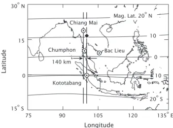
The magnetic equator runs mostly over the ocean as shown in Fig. 1, and it is not very easy to find suitable loca-tions to observe the ionosphere along the magnetic merid-ian. In the Southeast Asian area, the Indochinese Penin-sula lies to the north of the magnetic equator and the In-donesian Archipelago to the south. We established an iono-spheric observation network in this area (SEALION: South-east Asia low-latitude ionospheric network). Three ionoson-des composing a meridional chain along the 100◦E meridian were installed at Chiang Mai, a city in northern Thailand, at Chumphon, in the middle of the Malay Peninsula, and at Kototabang in West Sumatra, Indonesia (Fig. 2). Chumphon is slightly north of the magnetic equator (magnetic latitude is 3.3◦N). Kototabang is almost at the geographic equator (0.2◦S), and an atmospheric observation facility including the Equatorial Atmosphere Radar (EAR) is in the same ob-servation field. A combined use of the ionosonde and EAR data in the ionospheric irregularity study is described by Fukao et al. (2006). The magnetic latitude of Kototabang is 10.0◦S, and its magnetic conjugate point is at (100.1◦E, 16.6◦N). Chiang Mai was selected as a site close to the mag-netic conjugate of Kototabang. All stations are within 1.4◦ in longitude, and two magnetic meridians passing over Chi-ang Mai and KototabChi-ang are separated by 140 km at the F region height. The fourth station was installed in the
south-0 15 15o S 30oN 0 10 Mag. Lat. 20o N 10 20o S 90 75 105 120 135o E Longitude Latitude Chiang Mai Chumphon Kototabang Bac Lieu 140 km
Fig. 2. Southeast Asia low-latitude ionospheric network (SEALION). The conjugate point of Kototabang is indicated with the closed diamond.
ernmost area of Vietnam, Bac Lieu, near the magnetic equa-tor (magnetic latitude is 1.7◦N). The two meridians passing over Chumphon and Bac Lieu are separated by 740 km at the F region height. The parameters for the stations are summa-rized in Table 1.
In order to conduct continuous observations, we devel-oped a frequency modulated-continuous wave (FM-CW) ionosonde, which operates from 2 to 30 MHz with low elec-tric power. A commercial power amplifier module delivers a maximum power of 150 W. The prototype of the ionosonde is described by Nozaki and Kikuchi (1987).
1572 T. Maruyama et al.: Low latitude ionosphere-thermosphere dynamics studies
Table 1. Parameters for SEALION ionosonde stations.
Geographic location Conjugate point Station Longitude Latitude mag. lat. Longitude Latitude Chiang Mai 98.9◦ 18.8◦ 13.0◦ 99.2◦ −2.3◦ Chumphon 99.4◦ 10.7◦ 3.3◦ 99.4◦ 5.6◦ Kototabang 100.3◦ −0.2◦ −10.0◦ 100.1◦ 16.6◦ Bac Lieu 105.7◦ 9.3◦ 1.7◦ 105.7◦ 6.7◦ 500 400 300 200 100 Height, km 500 400 300 200 100 500 400 300 200 100 500 400 300 200 100 Height, km -20 -10 0 10 20 Latitude, deg. -20 -10 0 10 20 -20 -10 0 10 20 -20 -10 0 10 20 Latitude, deg. (a) (c) (b) (d)
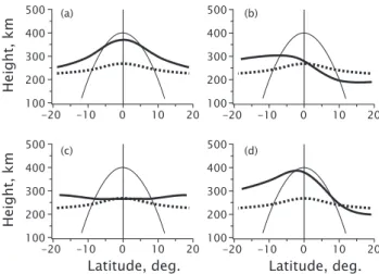
Fig. 3. Latitudinal variation in the bottom height of the ionosphere.
In each panel, the dotted line was obtained without external forces and the thin line indicates the magnetic field line across the equa-tor at 400 km. The thick lines represent changes in the bottom height caused by an upward E×B drift (a), a uniform transequato-rial northward wind (b), a convergence (with respect to the magnetic equator) neutral wind (c), and a combination of the upward E×B drift and the uniform transequatorial northward wind (d). The neg-ative sign of the latitude indicates the Southern Hemisphere.
3 Expected height variation at equatorial latitudes Ionospheric height variations are often discussed in terms of the F2-layer peak height (Rishbeth et al., 1978; Bittencourt and Sahai, 1978; Miller et al., 1986; Richards, 1991). The peak height can be calculated through a real height analysis (e.g., Titheridge, 1988) or formulations using the ionospheric transmission factor M(3000)F2 (Shimazaki, 1955; Berkey and Stonehocker, 1989). However, it was sometimes diffi-cult to scale the whole ionogram trace accurately, especially near the critical frequency. Another parameter representing the ionospheric height is the ionospheric virtual height, h′F , which can be directly and easily scaled from an ionogram. This is a good indicator of the bottom height of the iono-sphere in the night when solar radiation does not cause new ionization. In this paper, we discuss the ionospheric height in terms of the virtual height. However, we must be careful in using h′F as a height parameter; when the layer height
is largely depressed, the recombination effect overcomes the dynamical effect on the bottom height, and changes in h′F
do not necessarily reflect actual layer movements correctly. Although ionospheric height variations strongly reflect ex-ternal forces such as thermospheric neutral winds and zonal electric fields, these forces are difficult to separate from ionosonde observations alone. We examined the individual effects through model calculations for idealized situations. The model calculations solve the continuity and momentum equations (e.g., Maruyama, 1988) for equinox, medium solar activity (F10.7 solar flux is 100) conditions with a centered dipole magnetic field geometry. As described below, the as-sumption of forcing is overly simplified and the calculated features do not provide qualitative new information, but are expected theoretically. However, they should be helpful to demonstrate the ionospheric response to external forces for interpreting the observational results.
We calculated the ionospheric bottom height correspond-ing to the electron density of 7.75×104cm−3 (plasma fre-quency of 2.5 MHz) at 20:00 LT. The first run contained no external forcing, and the height was determined by chemical and diffusion processes alone. The result is shown in Fig. 3 by dotted lines, and is used as a reference curve in the all pan-els. The bottom height appears to be uplifted at the magnetic equator, and it gradually reaches a constant height as it leaves the equator. This is owing to the changes in the geometry of the magnetic flux tube. At low latitudes, plasma would be supplied from higher altitudes along the magnetic field line and the recombination losses would be somewhat compen-sated. However, at the magnetic equator, such replenishment across the magnetic field lines does not exist.
The second run examined the effect of an upward E×B drift, and the result is shown by the thick solid line in Fig. 3a. In this run, an electric field corresponding to 30 m/s at the magnetic equator was imposed at 19:00 LT and persisted for one hour. Through this upward E×B drift, the bottom height is raised by about 102 km at the magnetic equator, which is close to the actual displacement of the magnetic flux tube (108 km). On the other hand, at the latitude of 10◦, the uplift is only about 38 km, because of the downward diffu-sion imposed by the fountain effect. The third run examined the effect of a transequatorial neutral wind, and the result is shown by the thick solid line in Fig. 3b. In this run, a
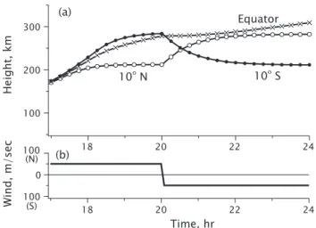
uniform northward neutral wind at the speed of 100 m/s was imposed at 19:00 LT and persisted for one hour. The bottom height at the magnetic equator is uplifted by about 10 km by the blow away effect (Maruyama, 1996). At 10◦in the windward hemisphere, the bottom height is uplifted by about 60 km, while in the other hemisphere, the bottom height is depressed by about 43 km. The relatively small (negative) perturbation compared with the windward hemisphere is the recombination effect which is significant in the lowered iono-sphere. A noticeable feature is that the bottom heights at low latitudes in the windward hemisphere are higher than at the magnetic equator. Figure 3c shows the effect of a con-vergence neutral wind. In this run, equatorward winds had amplitudes of 30 m/s at 10◦ in both hemispheres and lin-early decreased with lower latitude. The bottom height at the magnetic equator is the lowest. The last run (Fig. 3d) used the upward E×B drift model used for the second run and the neutral wind model used for the third run (transequa-torial mode wind). The bottom height difference between the Northern and Southern Hemispheres at 10◦is about 100 km, which is nearly the same as for run 3 (60+43 km) with only the neutral wind effect (Fig. 3b). This result indicates that the height difference caused by transequatorial winds is not strongly affected by the amplitude of the upward E×B drift. In the above, external forces were imposed at 19:00 LT, and the bottom height responses at 20:00 LT are described. However, the response is a function of time. Figure 4 shows how quickly the bottom height responds to the force. In this run, northward transequatorial wind turned southward at 20:00 LT, with the same amplitude (50 m/s). The north/south asymmetry of the height disturbance reversed about 30 min after the wind turned direction, and the time constant of the height response to the wind is around one hour.
4 Preliminary observational results
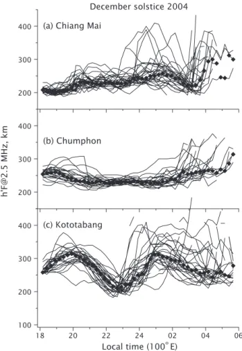
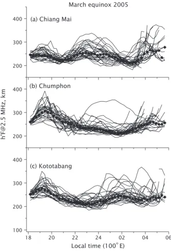
The first complete set of observations for the solstitial con-dition from the meridional chain was available in December 2004. Virtual heights at 2.5 MHz were scaled from the iono-gram with a 15-min interval, and the results for nighttime are plotted in Figs. 5a to c for Chiang Mai, Chumphon, and Ko-totabang, respectively, for the period from 7 December 2004 to 5 January 2005 (December solstice). Data for individual nights are shown by thin lines, and the median values of the period are shown by diamonds. The number of data points was greatly reduced after about 04:00 LT, because foF2 is close to or lower than 2.5 MHz, and the reliability of the data after that is low. The layer heights at the low-latitude sta-tions, Chiang Mai and Kototabang, after 23:00 LT exhibit a large day-to-day variability. The values at the equatorial station, Chumphon, are somewhat smaller than the values at the low-latitudes, which suggests that the variability at low latitudes mostly originated from a neutral wind effect, but not from a zonal electric field effect. On the other hand,
300 200 100 Height, km 24 22 20 18 10o N 10o S Equator 0 100 100 Wind, m/sec 18 20 22 24 Time, hr (a) (b) (N) (S)
Fig. 4. Response of the bottom height of the ionosphere to the meridional wind change at the magnetic equator and at 10◦
north and south of the magnetic equator (upper panel). The uni-form transequatorial wind turned from northward to southward at 20:00 LT (lower panel).
the Chumphon data shows a moderate day-to-day variabil-ity around 20:00 LT, which originated from the variabilvariabil-ity of the evening enhancement of the zonal electric field.
As the layer height at Chumphon is mostly controlled by the zonal electric field, the high layer height at Kototabang seen in the median plot, which peaked at 21:15 LT, and the low layer height at Chiang Mai are considered to be effects of northward neutral wind, as demonstrated in Fig. 3b. For a more detailed comparison, we obtained no-wind heights at Chiang Mai and Kototabang, with the aid of the model cal-culation described in the previous section, but for the tilted-dipole geometry and the day number of 356. First, the E×B drift velocity was adjusted to reproduce the height change at Chumphon. Then, the electron density distribution in the magnetic meridional plane was obtained. The difference be-tween the observed median values and the modeled heights at Chiang Mai and Kototabang are shown in Fig. 6a. Before 18:30 LT, h′F is affected by the propagation retardation in the lower part of the ionosphere, and the observation data are not compared with the modeled heights here. After sunset, the layer height at Kototabang was higher than the no-wind height and the layer at Chiang Mai was lower than the no-wind height. That is, transequatorial northward no-wind is pre-dominant, as mentioned above. As time elapsed, the height at Kototabang increased farther, but the height at Chiang Mai reached the no-wind height, and after 20:00 LT, the heights at Chiang Mai and Kototabang eventually became higher than the no-wind height. There could be two cases in which the layer height increases at both conjugate points: upward
E×B drift (Fig. 3a) and convergence wind (Fig. 3c).
How-ever, the E×B drift effect was already included in the model calculations by fitting the height variations at Chumphon. Thus, Fig. 6a indicates that the convergence-mode wind
1574 T. Maruyama et al.: Low latitude ionosphere-thermosphere dynamics studies
(a) Chiang Mai
400 300 200 (b) Chumphon 400 300 200 h'F@2.5 MHz, km (c) Kototabang 06 04 02 24 22 20 18 Local time (100o E) 400 300 200 100 December solstice 2004
Fig. 5. Virtual height at 2.5 MHz at Chiang Mai (a), Chumphon (b), and Kototabang (c) for the period from 7 December 2004 to
5 January 2005 (December solstice). Solid lines are for individual days and diamonds are monthly median values.
gradually intensified while the transequatorial-mode wind stayed the same. After 20:00 LT, the height at Kototabang decreased, but the height at Chiang Mai stayed at a mod-erately high level. That is, the transequatorial-mode wind weakened and the weak convergence-mode wind remained. At 22:00 LT, the height deviations at Kototabang and Chi-ang Mai reversed, or the transequatorial component reversed. A reversal of the transequatorial component occurred again at around 00:00 LT. Regarding the convergence/divergence mode, it vanished at 22:30 LT (equal height deviations but with a different sign). The convergence-mode wind in-creased again and reached a maximum at around 01:00 LT. As mentioned already, the response of the layer height to the neutral wind is delayed by half to one hour, and the actual times of the wind direction reversal should be earlier than in the above discussion.
It would be worthwhile to compare the observations with an empirical thermospheric wind model, HWM93 (Hedin et al., 1991), which is widely used to predict thermospheric
-50 0 50 100 KT CM ∆ h'F, km D-solstice 2004 Reference: No-wind -50 0 50 06 04 02 24 22 20 18 Local time (100o E) KT CM ∆ h'F, km Reference: HWM93-wind (a) (b)
Northward Southward Northward Southward
Convergence Convergence
Fig. 6. Deviation of the observed bottom height (monthly median)
from the modeled reference height without wind effect (a) and with the HWM93 wind model (b) for Kototabang (KT) and Chiang Mai (CM). In the lower part of panel (a), the meridional neutral wind inferable from the height deviations is shown.
wind fields. For this purpose, we ran another model calcula-tion which incorporated HWM93 and re-adjusted the E×B drift velocity. (The E×B drift velocity is slightly different from that obtained for the no-wind case, because Chumphon is not exactly at the magnetic equator.) The difference be-tween the observed median value and the modeled height is shown in Fig. 6b. The large deviation of h′F at Kotota-bang at around 20:00 LT is reduced to some extent when the HWM93 wind is assumed, but still there is a large discrep-ancy between the observations and the model results. The second peak of 1h′F for Kototabang at around 01:00 LT does not change very much even if the HWM93 wind field is taken into account. The most noteworthy feature in Fig. 6b is the periodic 5-h variation in 1h′F for both Kototabang and Chiang Mai. Such a higher order variation is not repre-sented in HWM93 (Hedin et al., 1991); yet the higher order variation is quite significant, especially after midnight at Ko-totabang, the geographic equator.
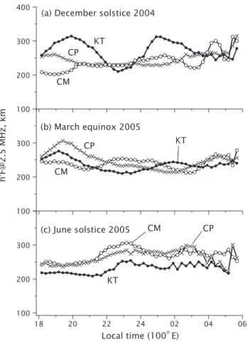
The neutral wind field is subject to variation with the lat-itude of the sub-solar point. Figures 7 and 8 show height variations for the March equinox (5 March 2005 to 5 April 2005) and the June solstice (5 June to 7 July 2005), respec-tively. As in Fig. 5, individual nights (thin lines) and me-dian values of the period (diamonds) are shown for the three stations. Median values for each period are reproduced in Fig. 9 along with those for the December solstice. At equinox (Fig. 9b), around 19:30 LT, the layer height at Chumphon
Local time (100o E) (c) Kototabang 06 04 02 24 22 20 18 400 300 200 100 (b) Chumphon 400 300 200 h'F@2.5 MHz, km
(a) Chiang Mai
400
300
200
March equinox 2005
Fig. 7. The same as Fig. 5 but for the period from 5 March to 5
April 2005 (March equinox).
(crosses) was largely enhanced compared with the other sea-sons. This is owing to an intense prereversal enhancement of the zonal electric field, which is known to be large dur-ing the equinox (Fejer et al., 1995). In contrast, the height at the low latitude stations, Chiang Mai, and Kototabang, was lower than at the equator, as expected from the small sea-sonal or transequatorial wind. A notable periodic change of about 6 h is clearly seen in the difference between the heights at Chiang Mai and Kototabang, similar to the one in Fig. 6 for the December solstice. That is, the transequatorial neu-tral wind periodically reversed northward and southward. At the June solstice, the layer height at Chiang Mai was higher than at Kototabang throughout the night, indicating south-ward transequatorial winds due to northsouth-ward migration of the sub-solar point. However, the pattern of the height variation was not quite the reverse of the December solstice, nor were there variations with 5–6 h.
Local time (100o E) (a) Chiang Mai
400 300 200 (b) Chumphon 400 300 200 h'F@2.5 MHz, km (c) Kototabang 06 04 02 24 22 20 18 400 300 200 100 June solstice 2005
Fig. 8. The same as Fig. 5 but for the period from 5 June to 7 July
2005 (June solstice).
5 Summary
The equatorial and low latitude ionosphere exhibits unique dynamical features stemming from strong north-south cou-pling and equally strong thermospheric wind and zonal elec-tric field effects. We established an ionosonde network in Southeast Asia that consists of four stations. Three of them form a meridional chain at 100◦E, at the magnetic conju-gate points and the magnetic equator. Another station is near the magnetic equator and is about 730 km east of the merid-ional chain. The study demonstrated that the meridional chain of ionosonde stations is advantageous for studying the ionosphere-thermosphere coupling. By scaling the virtual height from ionograms, nighttime ionospheric height vari-ations were analyzed. The seasonal trend of the inferred transequatorial-mode wind is generally reasonable, show-ing that the wind is directed from the summer to the winter hemispheres. The results were compared with theoretically calculated height variations incorporating an empirical ther-mospheric wind model, HWM93. The observed meridional wind exhibits a variation with a 5–6 h period, which is not
1576 T. Maruyama et al.: Low latitude ionosphere-thermosphere dynamics studies Local time (100o E) (b) March equinox 2005 300 200 100 h 'F @ 2 .5 M H z , k m (c) June solstice 2005 06 04 02 24 22 20 18 300 200 100
(a) December solstice 2004
100 400 300 200 KT KT KT CP CP CP CM CM CM
Fig. 9. Median values for the December solstice (a), March equinox (b), and June solstice (c) for Chiang Mai (CM), Chumphon (CP),
and Kototabang (KT).
represented by the existing empirical wind model and the amplitude is significant during the December solstice. The importance of such a variable wind field in the thermosphere-ionosphere system, including plasma instabilities and onsets of plasma bubbles, should be analyzed further. The day-to-day variability of ionospheric height and its relationship to onsets of equatorial spread F are given elsewhere (Saito and Maruyama, 2006). The preliminary analysis presented here is limited to the nighttime because we used directly scaled virtual heights, which are a good indicator of the layer height only in the nighttime. Peak height analysis using the iono-spheric transmission factor M(3000)F2 and foF2 (Shimazaki, 1955; Berkey and Stonehocker, 1989) would be a more uni-versal means, and will be a future topic. Also, the present analysis is on one-month median values in which possible local disturbances such as traveling ionospheric disturbances (Kelley et al., 1981) are smoothed out. The equatorial pair of Chumphon and Bac Lieu have the potential for a more detailed analysis based on a day-to-day values.
Acknowledgements. We are grateful to M. Yamamoto and S. Fukao
of Kyoto University, Japan and the staff of the National Institute of Aeronautics and Space, Indonesia (LAPAN) for installation of the
ionosonde and utilization of Equatorial Atmosphere Radar facility at Kototabang, Indonesia.
Topical Editor M. Pinnock thanks two anonymous referees for their help in evaluating this paper.
References
Abdu, M. A., Batista, I. S., Reinisch, B. W., and Carrasco, A. J.: Equatorial F-layer heights, evening prereversal electric field, and night E-layer density in the American sector: IRI validation with observations, Adv. Space Res., 34, 1953–1965, 2004.
Anderson, D. N.: A theoretical study of the ionospheric F region equatorial anomaly -2. Results in the American and Asian sec-tors, Planet. Space Sci., 21, 421–442, 1973.
Berkey, F. T. and Stonehocker, G. H.: A comparison of the height of the maximum electron density of the F2-layer from real height analysis and estimates based on M(3000)F2, J. Atmos. Terr. Phys., 51, 873–877, 1989.
Bittencourt, J. A. and Sahai, Y.: F-region neutral winds from ionosonde measurements of hmF2 at low latitude magnetic con-jugate regions, J. Atmos. Terr. Phys., 40, 669–676, 1978. Buonsanto, M. J.: Seasonal variations of day-time ionization flows
inferred from a comparison of calculated and observed NmF2, J. Atmos. Terr. Phys., 48, 365–373, 1986.
Chapman, S.: The absorption and dissociative or ionizing effect of monochromatic radiation in an atmosphere on a rotating earth, Proc. Phys. Soc., 43, 26–45, 1931.
de Medeiros, R. T., Abdu, M. A., and Batista, I. S.: Thermospheric meridional wind at low latitude from measurements of F layer peak height, J. Geophys. Res., 102(A7), 14 531–14 540, 1997. Farley, D. T., Bonelli, E., Fejer, B. G., and Larsen, M. F.: The
pre-reversal enhancement of the zonal electric field in the equatorial ionosphere, J. Geophys. Res., 91(A12), 13 723–13 728, 1986. Fejer, B. G., de Paula, E. R., Heelis, R. A., and Hanson, W. B.:
Global equatorial ionospheric vertical plasma drifts measured by the AE-E satellite, J. Geophys. Res., 100(A4), 5769–5776, 1995. Fukao, S., Yokoyama, T., Tayama, T. Yamamoto, M., Maruyama, T., and Saito, S.: Eastward traverse of equatorial plasma plumes observed with the Equatorial Atmosphere Radar in Indonesia, Ann. Geophys., 24, 1411–1418, 2006,
http://www.ann-geophys.net/24/1411/2006/.
Hanson, W. B. and Moffett, R. J.: Ionization transport effects in the equatorial F region, J. Geophys. Res., 71, 5559–5572, 1966. Hedin, A. E., Biondi, M. A., Burnside, R. G., et al.: Revised global
model of thermosphere winds using satellite and ground-based observations, J. Geophys. Res., 96(A5), 7657–7688, 1991. Heelis, R. A., Kendall, P. C., Moffett, R. J., Windle, D. W., and
Rishbeth, H.: Electrical coupling of the E- and F-regions and its effect on F-region drifts and winds, Planet. Space Sci., 22, 743– 756, 1974.
Igi, S., Ogawa, T., Oliver, W. L., and Fukao, S.: Thermospheric winds over Japan: Comparison of ionosonde and radar measure-ments, J. Geophys. Res., 100,(A11), 21 323–21 326, 1995. Kelley, M. C., Larsen, M. F., La Hoz, C., and McClure, J. P.:
Grav-ity wave initiation of equatorial spread F: A case study, J. Geo-phys. Res., 86(A11), 9087–9100, 1981.
Liu, L., Luan, X., Wan, W., Ning, B., and Lei, J.: A new approach to the derivation of dynamic information from ionosonde
surements, Ann. Geophys., 21, 2185–2191, 2003, http://www.ann-geophys.net/21/2185/2003/.
Maruyama, T.: A diagnostic model for equatorial spread F, 1. Model description and application to electric field and neutral wind ef-fects, J. Geophys., Res., 93(A12), 14 611–14 622, 1988. Maruyama, T.: Modeling study of equatorial ionospheric height
and spread F occurrence, J. Geophys. Res., 101(A3), 5157–5163, 1996.
Maruyama, T. and Matuura, N.: Longitudinal variability of annual changes in activity of equatorial spread F and plasma bubbles, J. Geophys. Res., 89(A12), 10 903–10 912, 1984.
Matuura, N.: Electric fields deduced from the thermospheric model, J. Geophys. Res., 79, 4679–4689, 1974.
Mendillo, M., Baumgardner, J., Pi, X., Sultan, P. J., and Tsunoda, R.: Onset conditions for equatorial spread F, J. Geophys. Res., 97(A9), 13 865–13 876, 1992.
Miller, K. L., Torr, D. G., and Richards, P. G.: Meridional winds in the thermosphere derived from measurement of F2 layer height, J. Geophys. Res., 91(A4), 4531–4535, 1986.
Miller, K. L., Salah, J. E., and Torr, D. G.: The effect of electric fields on measurements of meridional neutral winds in the ther-mosphere, Ann. Geophys., 5, 337–342, 1987,
http://www.ann-geophys.net/5/337/1987/.
Miller, K. L., Lemon, M., and Richards, P. G.: A meridional wind climatology from a fast model for the derivation of meridional winds from the height of the ionospheric F2 region, J. Atmos. Solar-Terr. Phys., 59, 1805–1822, 1997.
Namba, S. and Maeda, K.: Radio wave propagation, Corona Pub-lishing, Tokyo, p. 86, 1939.
Nozaki, K. and Kikuchi, T.: A new multimode FM/CW ionosonde, Mem. Natl. Inst. Polar Res., Special Issue, 47, 217–224, 1987. Reinisch, B. W., Abdu, M., Batista, I., Sales, G. S., Khmyrov, G.,
Bullett, T. A., Chau, J., and Rios, V.: Multistation digisonde ob-servations of equatorial spread F in South America, Ann. Geo-phys., 22, 3145–3153, 2004,
http://www.ann-geophys.net/22/3145/2004/.
Richards, P. G.: An improved algorithm for determining neutral winds from the height of the F2 peak electron density, J. Geo-phys. Res., 96(A10), 17 839–17 846, 1991.
Rishbeth, H., Ganguly, S., and Walker, J. C. G.: Field-aligned and field-perpendicular velocities in the ionospheric F2-layer, J. At-mos. Terr. Phys., 40, 767–784, 1978.
Rishbeth, H.: The equatorial F-layer: Progress and puzzles, Ann. Geophys., 18, 730–739, 2000,
http://www.ann-geophys.net/18/730/2000/.
Saito, S. and Maruyama, T.: Ionospheric height variations observed by ionosondes along magnetic meridian and plasma bubble on-sets, Ann. Geophys., 24, 2991–2996, 2006,
http://www.ann-geophys.net/24/2991/2006/.
Sharma, R. P. and Hewens, E. J.: A study of the equatorial anomaly at American longitudes during sunspot minimum, J. Atmos. Terr. Phys., 38, 475–484, 1976.
Shimazaki, T.: World-wide daily variations in the height of the max-imum electron density of the ionospheric F2 layer, J. Radio Res. Labs., 2, 85–97, 1955.
Strobel, D. F. and McElroy, M. B.: The F2-layer at middle latitudes, Planet. Space Sci., 18, 1181–1202, 1970.
Tanaka, T. and Hirao, K.: Effects of an electric field on the dynam-ical behavior of the ionospheres and its application to the storm time disturbance of the F-layer, J. Atmos. Terr. Phys., 35, 1443– 1452, 1973.
Titheridge, J. E.: The real height analysis of ionograms: A general-ized formulation, Radio Sci., 23, 831–849, 1988.
Titheridge, J. E.: The calculation of neutral winds from ionospheric data, J. Atmos. Terr. Phys., 57, 1015–1036, 1995.
Walker, G. O. and Chan, H. F.: Computer simulations of the sea-sonal variations of the ionospheric equatorial anomaly in East Asia under solar minimum conditions, J. Atmos. Terr. Phys., 51, 953–974, 1989.
Yonezawa, T.: Theory of formation of the ionosphere, Space Sci. Rev., 5, 3–56, 1966.