Altitude dependence of plasma density in the auroral zone

HAL Id: hal-00317370

https://hal.archives-ouvertes.fr/hal-00317370

Submitted on 1 Jan 2002

HAL is a multi-disciplinary open access

archive for the deposit and dissemination of

sci-entific research documents, whether they are

pub-lished or not. The documents may come from

teaching and research institutions in France or

abroad, or from public or private research centers.

L’archive ouverte pluridisciplinaire HAL, est

destinée au dépôt et à la diffusion de documents

scientifiques de niveau recherche, publiés ou non,

émanant des établissements d’enseignement et de

recherche français ou étrangers, des laboratoires

publics ou privés.

Altitude dependence of plasma density in the auroral

zone

P. Janhunen, A. Olsson, H. Laakso

To cite this version:

P. Janhunen, A. Olsson, H. Laakso. Altitude dependence of plasma density in the auroral zone.

Annales Geophysicae, European Geosciences Union, 2002, 20 (11), pp.1743-1750. �hal-00317370�

Annales

Geophysicae

Altitude dependence of plasma density in the auroral zone

1_{Finnish Meteorological Institute, Geophysical Research, Helsinki, Finland} 2_{Swedish Institute of Space Physics, Uppsala Division, Uppsala, Sweden} 3_{ESTEC, Space Science Department, Noordwijk, The Netherlands}

Received: 21 February 2002 – Revised: 5 June 2002 – Accepted: 2 July 2002

Abstract. We study the altitude dependence of plasma

deple-tions above the auroral region in the 5000–30 000 km altitude range using five years of Polar spacecraft potential data. We find that besides a general decrease of plasma density with altitude, there frequently exist additional density depletions at 2–4 REradial distance, where REis the Earth radius. The

position of the depletions tends to move to higher altitude when the ionospheric footpoint is sunlit as compared to dark-ness. Apart from these cavities at 2–4 RE radial distance,

separate cavities above 4 REoccur in the midnight sector for

all Kp and also in the morning sector for high Kp. In the

evening sector our data remain inconclusive in this respect. This holds for the ILAT range 68–74. These additional de-pletions may be substorm-related. Our study shows that au-roral phenomena modify the plasma density in the auau-roral region in such a way that a nontrivial and interesting altitude variation results, which reflects the nature of the auroral ac-celeration processes.

Key words. Magnetospheric physics (auroral phenomena;

magnetosphere–ionosphere interactions)

1 Introduction

Plasma density appears to be considerably variable in the au-roral zone. While crossing that region, satellites commonly observe deep density depletions of various spatial and tem-poral scales. In this paper we use the word cavity as meaning the same as a density depletion, i.e., an occurrence of low plasma density in an absolute sense, without regard to how spatially or temporally localized it is. In addition to iono-spheric plasma density depletions (Doe et al., 1993), den-sity depletions often occur in the nightside auroral region at a few thousand kilometer altitudes (Benson and Calvert, 1979; Calvert, 1981) and above (Persoon et al., 1988). There is a correlation between the depletions and upflowing ions and precipitating auroral electrons (Persoon et al., 1988;

Per-Correspondence to: P. Janhunen (Pekka.janhunen@fmi.fi)

soon, 1988), thus the density depletions are probably inti-mately related to the inverted-V and auroral arc formation as has also been demonstrated using simulations (e.g. Ergun et al., 2000). The density depletions are also suggested to be the source regions of the auroral kilometric radiation (AKR) (Strangeway et al., 2001). The association with inverted-V phenomena whose scale sizes are usually less than 100 km is also in line with the facts that the deepest depletions typically have scale sizes less than 100 km (Hilgers, 1992) and that these depletions are most common in the nightside. Density depletions of more than 40% of the background density are observed in 70% of the nightside crossings of DE-1 (Persoon et al., 1988). Density depletions with AKR are often stable for at least several tens of minutes (Bahnsen et al., 1989).

The purpose of this paper is to study statistically the al-titude variation (1.5–6 RE radial distance, where by radial

distance we mean the direct distance from the center of the Earth) of plasma density in the auroral zone, using five years (1996–2001) of spacecraft potential data from the Electric Field Investigation (EFI) onboard Polar (Harvey et al., 1995). We will study this density variation as a function of magnetic local time (MLT) sectors, invariant latitude (ILAT), Kpindex

and solar illumination. A statistical study on auroral density depletions at 1 REaltitude has been published recently, using

one year of measurements by the same instrument (Johnson et al., 2001).

2 Observations

The basic principle of using the spacecraft potential for studying plasma density variations is as follows (Pedersen, 1995; Laakso and Pedersen, 1998; Johnson et al., 2001): when a satellite, immersed in a tenuous plasma (density be-low 1000 cm−3), is illuminated by the Sun, continuous pho-toelectron emission from the surface of the spacecraft causes the satellite to become positively charged with respect to the surrounding plasma. An equilibrium is reached when the thermal flux of electrons from the surrounding plasma equals

1744 P. Janhunen et al.: Auroral plasma density the photoelectron flux. It can be shown that the spacecraft

potential is larger (more positive) when the plasma density is small. The exact relationship between the spacecraft poten-tial and the density remains uncertain because it depends on the details of the photoelectron energy spectrum and thus on the properties of the satellite surface material and solar spec-trum, although one can calibrate the relationship by using comparisons with more direct ways to calculate the plasma density (Scudder et al., 2000). In the present study we as-sume that a spacecraft potential versus density relationship exists, but knowing the relationship in detail is not necessary to draw our conclusions.

In this study we use the Polar/EFI spacecraft potential measurements, sampled at 2.5 times per second. To keep the statistical analysis to a manageable size we take every 30th sample of the raw data, thus yielding one data point every 12 s. We follow the usual convention and always display the negative of the spacecraft potential. Eclipse periods are re-moved because in those the spacecraft potential is not an in-dicator of plasma density. We call the negative of the space-craft potential VSC, measured in volts. To get information

about density variations we selected three threshold values for VSC: −11 V, −18 V and −25 V (corresponding to

densi-ties of roughly 0.3 cm−3, 0.1 cm−3and 0.06 cm−3, respec-tively (Scudder et al., 2000). However, our results are not sensitive to the calibration of the spacecraft potential versus density relationship because only relative changes are con-sidered. We only ask questions like what is the occurrence frequency of VSC < −11 V as a function of altitude etc.,

without having to know exactly what density value −11 V actually corresponds to.

In principle the spacecraft potential depends not only on density but also on electron temperature (Laakso and Peder-sen, 1998; Johnson et al., 2001). To evaluate this effect quan-titatively we use Eqs. (1)–(4) of Johnson et al. (2001) gen-eralizing them to the case of two Maxwellian electron pop-ulations, one representing the background plasma (the cold component) and the other, if any, representing the energetic plasma (the hot component). The Debye length needed in the shielding distance calculation in Eq. (2) of Johnson et al. (2001) is given by λDe = (λ−De21+λ

−2

De2)

−1/2 _{where λ}

De1

and λDe2are the cold and hot component Debye lengths,

re-spectively.

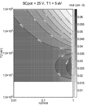
In Fig. 1 we show the density corresponding to a spacecraft potential value of −25 V, for varying mixtures of hot and cold plasma. The cold electron temperature is fixed and set to 5 eV, and the hot electron temperature is varied between 5 eV and 10 keV. The mixing ratio (hot density versus total density) is varied between 1% and 90%. When the electron temperatures are below some hundred electronvolts, the total density corresponding to −25 V is almost independent of the temperature and density mixing ratio and equal to about 0.05 cm−3(in the specific model of spacecraft and photoelectrons used by, Johnson et al., 2001). To reach 50% deviation from this total density value, i.e. density 0.025 cm−3, one should, for example, have 35% of 2 keV plasma.

Figure 2 is rather similar to Fig. 1, but now we keep the

0.01 0.1 1 1.0×100 1.0×101 1.0×102 1.0×103 1.0×104 SCpot = 25 V, T1 = 5 eV n2/ntot T2 (e V ) ntot (cm -3) 0.01 0.015 0.02 0.025 0.03 0.035 0.04 0.045 0.05 0.055 0.06 0.01₅ 0.02 0.02₅ 0.025 0.03 0.03 0.03₅ 0.03₅ 0.04 0.04 0.04₅ 0.045 0.045 0.05 0.05 0.05 5

Fig. 1. Density value corresponding to a spacecraft potential −25 V

in a model containing two Maxwellian electron populations, called hot and cold. The horizontal axis is the hot versus total density ratio and the vertical axis is the hot component temperature. The cold component temperature is set to 5 eV.

total density fixed at 0.05 cm−3 and plot the spacecraft po-tential for different hot temperatures and mixing ratios. From Figs. 1 and 2, we can draw the conclusion that for the given densities, the increase of the temperature of the hot compo-nent increases Vsc, as expected, but the change is not very dramatic unless we have only a hot population and its temper-ature approaches 1 keV and goes beyond that. More specif-ically, a region with 0.05 cm−3 density (a “deep” cavity), which normally should have the spacecraft potential about

−25 V, may have a spacecraft potential of only −18 V and thus be classified only “medium-deep” if it contains 20% of 10 keV electrons. In practice, the temperature should not have a significant effect on our statistical results, except per-haps within and below the bottom of the acceleration region (below 2–3 RE radial distance, depending on the solar

illu-mination condition of the footpoint ionosphere) where some cavities might be missed because of the abundance of high-energy inverted-V electrons.

We stress that although we for definiteness use a specific model (Johnson et al., 2001) to compute explicit density val-ues, we do not need the exact spacecraft potential versus den-sity relationship to reach the conclusions of this study, but only the relative changes of this relationship are of impor-tance.

0.01 0.1 1 1.0×100 1.0×101 1.0×102 1.0×103 1.0×104

ntot = 0.05 cm-3, T1 = 5 eV

Fig. 2. Spacecraft potential value corresponding to density 0.05

cm−3in a model containing two Maxwellian electron populations, called hot and cold. The horizontal axis is the hot versus total den-sity ratio and the vertical axis is the hot component temperature. The cold component temperature is set to 5 eV.

3 Results

For an overview, we show in Fig. 3 the dependence of cav-ity occurrence rate on MLT and ILAT for threshold values

−11 V, −18 V and −25 V. The occurrence rate is defined as the number of data points where the spacecraft potential is more negative than the given threshold, divided by the total number of data points in the R, MLT, ILAT, etc. bin in ques-tion. All radial distance bins, including measurements during all magnetic conditions, are put together in this plot. The or-bital coverage is also shown in the bottom panel. The occur-rence rate of large satellite potentials, or low plasma densi-ties, follows the general pattern of the auroral oval (Feldstein and Starkov, 1967) in the nightside MLT sectors. (In the day-side MLT sectors the mean oval is poleward of 74 ILAT and so cannot be seen in our plot). This result is in agreement with Johnson et al. (2001). The lowest densities (highest oc-currence rate for cavities) are found above ILAT 68.

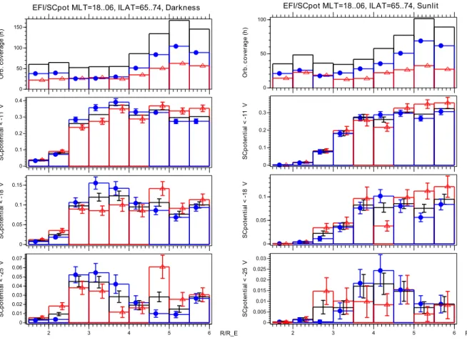
In Fig. 4 we show the occurrence frequencies of auroral cavities at 18:00–06:00 MLT sector for the cases where the ionospheric footpoint is in darkness (left subplot) or sun-illuminated (right subplot). Again, three different spacecraft potential thresholds are used (−11 V, −18 V and −25 V) rep-resenting shallow, medium-deep and deep cavities, respec-tively. Geomagnetic activity is binned into two groups so

65 66 67 68 69 70 71 72 73 IL A T SC po t < -1 1 V oc c. ra te 0 0.1 0.2 0.3 0.4 0.5 65 66 67 68 69 70 71 72 73 IL A T SC po t < -1 8 V oc c. ra te 0 0.05 0.1 0.15 0.2 0.25 65 66 67 68 69 70 71 72 73 IL A T SC po t < - 25 V oc c. ra te 0 0.01 0.02 0.03 0.04 0.05 0.06 0.07 0.08 0 5 10 15 20 MLT 65 66 67 68 69 70 71 72 73 IL A T O rb . c ov er ag e (h ) 0 10 20 30 40 EFI/SCpot R=1..6, All Kp

Fig. 3. Occurrence frequency of cavities for three different

thresh-olds as a function of MLT and ILAT. The lowest panel shows the orbital coverage.

that small Kpindex values (0 ≤ Kp ≤2) are shown by solid

lines with filled circles, large Kpindex values (Kp >2) by

solid lines with open triangles, and all Kp’s put together by

dotted lines with no symbol. The orbital coverage is also shown on the top. The occurrence frequency was first cal-culated separately for each ILAT bin (the ILAT bin width is 1◦_{), then linearly averaged over ILAT. Because of this, the}

results are not sensitive to possibly nonuniform ILAT cov-erage. Error bars are shown except when the error is in-significantly small. The error estimates are calculated from the number of orbital crossings visiting the (R, ILAT, MLT) bin. If the number of data points is N , the number of points satisfying the cavity threshold condition is n and the num-ber of orbital crossings contributing to the bin is K, the oc-currence frequency is f = n/N and its standard deviation

1f =√f (1 − f )/K. This method of error estimation con-siders measurements made during one orbital crossing within the bin as fully correlated. Thus it is likely that the true errors are somewhat smaller than our error bars.

From the second panels of Fig. 4 (shallow cavities, space-craft potential more negative than −11 V) we see that cavi-ties are rare, i.e., plasma densicavi-ties are on the average high, close to the Earth and that the region of higher plasma den-sities extends to a higher altitude when the ionospheric

foot-1746 P. Janhunen et al.: Auroral plasma density 0 50 100 150 O rb . c ov er ag e (h ) 0 0.1 0.2 0.3 0.4 SC po te nt ia l < -1 1 V 0 0.05 0.1 0.15 SC po te nt ia l < -1 8 V 2 3 4 5 6 R/R_E 0 0.01 0.02 0.03 0.04 0.05 0.06 0.07 SC po te nt ia l < -2 5 V

EFI/SCpot MLT=18..06, ILAT=65..74, Darkness

0 50 100 O rb . c ov er ag e (h ) 0 0.1 0.2 0.3 SC po te nt ia l < -1 1 V 0 0.05 0.1 SC po te nt ia l < -1 8 V 2 3 4 5 6 R/R_E 0 0.005 0.01 0.015 0.02 0.025 0.03 SC po te nt ia l < -2 5 V

EFI/SCpot MLT=18..06, ILAT=65..74, Sunlit

Fig. 4. Occurrence frequency of nightside auroral cavities for conditions when the ionospheric footpoint is in darkness (left subplot) and

sun-illuminated (right subplot). The top panel of each subplot is the orbital coverage in hours while the remaining panels give the occurrence frequency for spacecraft potential thresholds −11 V, −18 V and −25 V. Low Kp(≤ 2) is shown by blue lines with filled dots, high Kp(> 2)

by red lines and open triangles and all Kp’s put together by solid black line with no symbol. The horizontal axis in each subplot is the radial

distance from 1.5 to 6 RE. Error bars are shown except when they are insignificantly small. If the orbital coverage is less than 20 min, the

corresponding occurrence frequencies are not shown.

point is illuminated by the sun. The occurrence frequency of the shallow cavities is almost constant at higher altitudes. Deeper cavities (third and fourth panels) are, on the contrary, concentrated near a specific radial distance. The maximum occurrence frequency is at around 3.25 REradial distance for

darkness conditions and at 4.25 REfor sunlit conditions. The

solar illumination condition is calculated at the 110 km alti-tude. It thus seems that cavities of about 1–1.5 RE radial

extent tend to exist at this altitude and that their preferred altitude is lifted up by about 1 RE when the footpoint is

illu-minated by the sun. 3.1 Darkness conditions

Since the effect of solar illumination is seen to be impor-tant, we from now on separate all our statistics in dark-ness and sunlit conditions. In Fig. 5 we show an MLT and ILAT-decomposed view of the statistics. We have three 4-h MLT sectors (18:00–22:00, 22:00–02:00 and 02:00–06:00) and three 3-degree ILAT ranges (65–68◦, 68–71◦ and 71– 74◦). Notice that the scales are different for all panels due to

a large range of values.

The peak in occurrence frequency at around 3 REis seen

in many of the subplots of Fig. 5, especially in the pre-midnight sectors below 71◦, and it becomes clearer when the spacecraft potential threshold is made more negative (VSC < −18 V and VSC < −25 V). The occurrence rate of

cavities naturally becomes lower when the threshold is made more negative. Otherwise the altitude of the peak does not seem to depend on the threshold. Also, the peak altitude does not much depend on the Kpindex.

Comparison of different ILAT ranges (different rows in Fig. 5) shows that cavities are rare for low Kp for low ILAT

(65 . . . 68), especially in the evening and morning MLT sec-tors, while high Kp cavities are more common even for low

ILAT. This has been inferred earlier in the 2–4 REradial

dis-tance range from DE-1 (Persoon, 1988). A natural explana-tion for this is the expansion of the auroral oval to lower ILAT during disturbed conditions (Feldstein and Starkov, 1967).

The peak altitude is lower by 0.5 RE(residing at 2.75 RE

radial distance) in the midnight sector as compared to the morning sector (3.25 RE) if one looks at all Kp values and

0 5 10 15 O rb . c ov er ag e (h ) 0 0.1 0.2 0.3 0.4 0.5 0.6 0.7 0.8 0.9 SC po t < -1 1 V 0 0.1 0.2 0.3 0.4 0.5 0.6 SC po t < -1 8 V 2 3 4 5 6 R/R_E 0 0.1 0.2 0.3 0.4 0.5 SC po t < -2 5 V MLT=18..22, ILAT=71..74, Darkness 0 5 10 15 20 O rb . c ov er ag e (h ) 0 0.1 0.2 0.3 0.4 0.5 0.6 0.7 SC po t < -1 1 V 0 0.050.1 0.150.2 0.250.3 SC po t < -1 8 V 2 3 4 5 6 R/R_E 0 0.05 0.1 0.15 SC po t < -2 5 V MLT=22..02, ILAT=71..74, Darkness 0 5 10 15 O rb . c ov er ag e (h ) 0 0.1 0.2 0.3 0.4 0.5 0.6 0.7 0.8 SC po t < -1 1 V 0 0.1 0.2 0.3 0.4 SC po t < -1 8 V 2 3 4 5 6 R/R_E 0 0.05 0.1 0.15 SC po t < -2 5 V MLT=02..06, ILAT=71..74, Darkness 0 5 10 15 O rb . c ov er ag e (h ) 0 0.5 1 SC po t < -1 1 V 0 0.1 0.2 0.3 0.4 SC po t < -1 8 V 2 3 4 5 6 R/R_E 0 0.050.1 0.150.2 0.25 SC po t < -2 5 V MLT=18..22, ILAT=68..71, Darkness 0 5 10 15 20 O rb . c ov er ag e (h ) 0 0.1 0.2 0.3 0.4 0.5 0.6 SC po t < -1 1 V 0 0.050.1 0.150.2 0.25 SC po t < -1 8 V 2 3 4 5 6 R/R_E 0 0.05 0.1 SC po t < -2 5 V MLT=22..02, ILAT=68..71, Darkness 0 5 10 15 O rb . c ov er ag e (h ) 0 0.1 0.2 0.3 0.4 SC po t < -1 1 V 0 0.05 0.1 0.15 SC po t < -1 8 V 2 3 4 5 6 R/R_E 0 0.01 0.02 0.03 0.04 0.05 0.06 0.07 0.08 SC po t < -2 5 V MLT=02..06, ILAT=68..71, Darkness 0 5 10 15 O rb . c ov er ag e (h ) 0 0.1 0.2 0.3 SC po t < -1 1 V 0 0.05 0.1 0.15 0.2 SC po t < -1 8 V 2 3 4 5 6 R/R_E 0 0.05 0.1 0.15 SC po t < -2 5 V MLT=18..22, ILAT=65..68, Darkness 0 5 10 15 20 25 30 O rb . c ov er ag e (h ) 0 0.05 0.1 0.15 0.2 SC po t < -1 1 V 0 0.05 0.1 SC po t < -1 8 V 2 3 4 5 6 R/R_E 0 0.01 0.02 0.03 0.04 0.05 0.06 SC po t < -2 5 V MLT=22..02, ILAT=65..68, Darkness 0 5 10 15 20 25 O rb . c ov er ag e (h ) 0 0.05 0.1 SC po t < -1 1 V 0 0.01 0.02 0.03 0.04 0.05 SC po t < -1 8 V 2 3 4 5 6 R/R_E 0 0.0050.01 0.0150.02 0.0250.03 SC po t < -2 5 V MLT=02..06, ILAT=65..68, Darkness

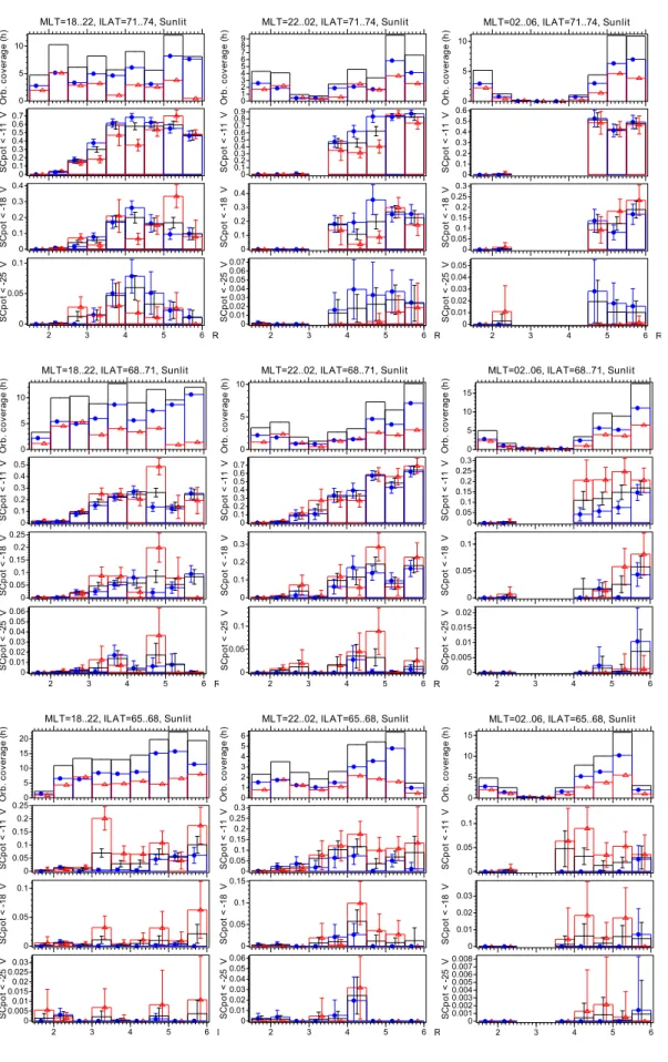
Fig. 5. Occurrence frequency of spacecraft potential being more negative than a threshold. Same format as Fig. 4 but for darkness conditions

only and decomposed into three MLT and three ILAT ranges. The MLT and ILAT ranges are shown in the title of each of the nine subplots. MLT changes along the rows and ILAT along the columns. As before, low Kpis shown by blue, high Kpas red and all Kp’s put together

1748 P. Janhunen et al.: Auroral plasma density 0 5 10 O rb . c ov er ag e (h ) 0 0.1 0.2 0.3 0.4 0.5 0.6 0.7 SC po t < -1 1 V 0 0.1 0.2 0.3 0.4 SC po t < -1 8 V 2 3 4 5 6 R/R_E 0 0.05 0.1 SC po t < -2 5 V MLT=18..22, ILAT=71..74, Sunlit 0 1 2 3 4 5 6 7 8 9 O rb . c ov er ag e (h ) 0 0.1 0.2 0.3 0.4 0.5 0.6 0.7 0.8 0.9 SC po t < -1 1 V 0 0.1 0.2 0.3 0.4 SC po t < -1 8 V 2 3 4 5 6 R/R_E 0 0.01 0.02 0.03 0.04 0.05 0.06 0.07 SC po t < -2 5 V MLT=22..02, ILAT=71..74, Sunlit 0 5 10 O rb . c ov er ag e (h ) 0 0.1 0.2 0.3 0.4 0.5 0.6 SC po t < -1 1 V 0 0.050.1 0.150.2 0.250.3 SC po t < -1 8 V 2 3 4 5 6 R/R_E 0 0.01 0.02 0.03 0.04 0.05 SC po t < -2 5 V MLT=02..06, ILAT=71..74, Sunlit 0 5 10 O rb . c ov er ag e (h ) 0 0.1 0.2 0.3 0.4 0.5 SC po t < -1 1 V 0 0.05 0.1 0.15 0.2 0.25 SC po t < -1 8 V 2 3 4 5 6 R/R_E 0 0.01 0.02 0.03 0.04 0.05 0.06 SC po t < -2 5 V MLT=18..22, ILAT=68..71, Sunlit 0 5 10 O rb . c ov er ag e (h ) 0 0.1 0.2 0.3 0.4 0.5 0.6 0.7 SC po t < -1 1 V 0 0.1 0.2 0.3 SC po t < -1 8 V 2 3 4 5 6 R/R_E 0 0.05 0.1 SC po t < -2 5 V MLT=22..02, ILAT=68..71, Sunlit 0 5 10 15 O rb . c ov er ag e (h ) 0 0.050.1 0.150.2 0.250.3 SC po t < -1 1 V 0 0.05 0.1 SC po t < -1 8 V 2 3 4 5 6 R/R_E 0 0.005 0.01 0.015 0.02 SC po t < -2 5 V MLT=02..06, ILAT=68..71, Sunlit 0 5 10 15 20 O rb . c ov er ag e (h ) 0 0.05 0.1 0.15 0.2 0.25 SC po t < -1 1 V 0 0.05 0.1 SC po t < -1 8 V 2 3 4 5 6 R/R_E 0 0.0050.01 0.0150.02 0.0250.03 SC po t < -2 5 V MLT=18..22, ILAT=65..68, Sunlit 0 1 2 3 4 5 6 O rb . c ov er ag e (h ) 0 0.050.1 0.150.2 0.250.3 SC po t < -1 1 V 0 0.05 0.1 0.15 SC po t < -1 8 V 2 3 4 5 6 R/R_E 0 0.01 0.02 0.03 0.04 0.05 0.06 SC po t < -2 5 V MLT=22..02, ILAT=65..68, Sunlit 0 5 10 15 O rb . c ov er ag e (h ) 0 0.05 0.1 SC po t < -1 1 V 0 0.01 0.02 0.03 SC po t < -1 8 V 2 3 4 5 6 R/R_E 0 0.001 0.002 0.003 0.004 0.005 0.006 0.007 0.008 SC po t < -2 5 V MLT=02..06, ILAT=65..68, Sunlit

at the medium-deep and deep cavities in which the peak is most clearly seen. For the evening sector we cannot make this comparison because of lack of orbital coverage. The tendency of deep cavities to occur only around 3 RE radial

distance if very strong for low ILAT (65 . . . 68).

Apart from the cavities occurring near 3 RE radial

dis-tance, there are more irregularly occurring cavities also at higher altitude, especially in the midnight sector, but also in the morning sector when the Kpindex is above 2 and when

ILAT ≥ 68. These high altitude cavities have a tendency of being separated from the lower altitude ones, e.g. in the mid-night sector (22 . . . 02) and in the main auroral oval ILAT (68 . . . 71) there are no deep cavities at all in the 3.75 RE

radial bin. Because of their MLT and Kp dependence, it

seems possible that these high-altitude cavities are substorm-related. To confirm this we would need better coverage in the evening sector, however.

3.2 Sunlit conditions

Figures 6 is similar to Fig. 5, but it describes sunlit condi-tions. The overall occurrence frequency of cavities is not much lower in sunlit conditions than in darkness, except for the deepest (−25 V) cavities. For sunlit conditions we have good coverage in the evening sector, but not so good in the midnight and morning sectors. In the evening sector there is a clearly defined island of cavities which is best visible in the

−25 V threshold and 71 . . . 74 ILAT bin. In this ILAT bin the island is centered at 4.25 REradial distance. For lower ILAT

the island altitude gets a bit lower and it becomes less regular. In the 65 . . . 68 ILAT bin there is no longer a clearly defined island, at least not for small Kp. We think that this island

of cavities is the same as the ∼ 3 RE occurrence frequency

peak seen in the darkness statistics, but which is now raised to higher altitude because of increased ionospheric plasma density. Because of incomplete orbital coverage we do not attempt to analyse to what extent the island exists in sunlit conditions in the midnight and morning MLT sectors.

4 Summary and discussion

Our statistical study of density depletions using Polar space-craft potential reveals the following main conclusions:

1. Cavities show an auroral zone dependency, which indi-cates that most of them are associated with auroral pro-cesses. The low-altitude (R ≈ 2RE) part of this result

has been found earlier (Johnson et al., 2001).

2. Cavities are raised to ∼ 1 RE higher altitude in sunlit

conditions as compared to darkness conditions. 3. In darkness, there is a peak in cavity occurrence

fre-quency at about 3.25 RE radial distance. The region of

cavities ends at about 4.25 RE, apart from the midnight

sector (see item 7 below). In sunlit conditions the maxi-mum is at 3.75 REand the region of cavities extends up

to 5.25 RE.

4. The peak is clearest for the deepest cavities.

5. The Kp index does not have a clear effect on the peak

altitude.

6. For low ILAT, cavities occur mainly only for large Kp,

probably because the auroral oval extends equatorward during disturbed conditions. For other ILAT, however, cavities are more common for low Kpthan for high Kp.

This has been inferred earlier in the 2–4 RE radial

dis-tance range from DE-1 (Persoon, 1988). A possible rea-son is that it takes time for an auroral arc-associated cav-ity to develop low densities, and under disturbed condi-tions, the arcs may move faster to a new location before a really deep cavity has been set up in the old location. 7. In the midnight sector there are cavities also in the 4–

6 RE radial distance range for both low and high Kp.

They also occur in the morning sector, but only for high

Kp. This holds for ILAT range 68–74. These cavities

may be related to substorms.

8. The influence of the electron energy on the spacecraft potential versus density relationship is such that in our statistics, some cavities might be missed within and be-low the bottom of the acceleration region (about 2–3 RE

radial distance, depending on whether the footpoint is sun-illuminated or not).

The overall behavior of the plasma density in the auro-ral zone in the 5000–30 000 km altitude range thus seems to be that (1) in general, density decreases with altitude, and (2) superposed on this basic trend, auroral density depletions occur, These density depletions have an upper boundary at

∼20 000 km altitude, in addition to having a lower boundary below ∼ 10 000 km altitude. As shown above, the average altitudes of the boundaries of the auroral density depletions depend on the solar illumination condition. This is natural, since the increased ionospheric plasma density during sun-lit conditions makes it harder to create deep cavities at low altitude.

Our results suggest that density cavities associated with auroral processes do not usually continue beyond 4 REradial

distance, except perhaps in substorm-related cases. Since auroral density cavities at low altitude are associated with auroral potential structures (Strangeway et al., 1998), they could also plausibly have a similar relationship with each other at higher altitude. In this light, the recent suggestion that auroral potential structures are primarily confined be-low 4 RE radial distance (Janhunen et al., 1999) is

consis-tent with the density cavity statistics presented here. In a recent work modelling the potential structure above an auro-ral arc (Janhunen and Olsson, 2000), an O-shaped potential together with a self-consistent maintenance mechanism was suggested. In this model, magnetospheric few hundred elec-tronvolt electrons would be repelled by a downward parallel electric field associated with the upper part of the potential structure. An electron cavity of similar shape as the potential

1750 P. Janhunen et al.: Auroral plasma density would thus be the result of this filtering effect. Ions would

move faster within the negative O-potential due to electro-static forces and thus their density would also be reduced, thus quasineutrality would remain. In other words, the model suggested by (Janhunen and Olsson, 2000) predicts an arc-associated density cavity to exist at a limited altitude range, which is in harmony with the statistical findings reported in the present paper.

Acknowledgements. We are grateful to Forrest S. Mozer for

provid-ing the EFI data. The work of PJ was supported by the Academy of Finland and that of AO by the Swedish Research Council.

Topical Editor G. Chanteur thanks two referees for their help in evaluating this paper.

References

Bahnsen, A., Pedersen, B. M., Jespersen, M., Ungstrup, E., Elias-son, L., Murphree, J. S., Elpinstone, R. D., Blomberg, L., Holm-gren, G., and Zanetti, L. J.: Viking observations at the source re-gion of auroral kilometric radiation, J. Geophys. Res., 94, 6643– 6654, 1989.

Benson, R. F. and Calvert, W.: ISIS 1 observations at the source of auroral kilometric radiation, J. Geophys. Res., 94, 6643–6654, 1989.

Calvert, W.: The auroral plasma cavity, Geophys. Res. Lett., 8, 919– 921, 1981.

Doe, R. A., Mendillo, M., Vickrey, J. F., Zanetti, L. J., and Eastes, R. W.: Observations of nightside auroral cavities, J. Geophys. Res., 98, 293–310, 1993.

Ergun, R. E., Carlson, C. W., McFadden, J. P., Mozer, F. S., and Strangeway, R. J.: Parallel electric fields in discrete arcs, Geo-phys. Res. Lett., 27, 4053–4056, 2000.

Feldstein, Y. I. and Starkov, G. V.: Dynamics of auroral belt and polar geomagnetic disturbances, Planet. Space Sci., 15, 209–229, 1967.

Harvey, P., et al.: The electric field instrument on the Polar satellite, Space Sci. Rev., 71, 583–596, 1995.

Hilgers, A.: The auroral radiating plasma cavities, Geophys. Res.

Lett., 19, 237–240, 1992.

Janhunen, P., Olsson, A., Mozer, F. S., and Laakso, H.: How does the U-shaped potential close above the acceleration region? A study using Polar data, Ann. Geophysicae, 17, 1276–1283, 1999. Janhunen, P. and Olsson, A.: New model for auroral acceleration: O-shaped potential structure cooperating with waves, Ann. Geo-physicae, 18, 596–607, 2000.

Johnson, M. T., Wygant, J. R., Cattell, C., Mozer, F. S., Temerin, M., and Scudder, J.: Observations of the seasonal dependence of the thermal plasma density in the southern hemisphere auro-ral zone and polar cap at 1 RE, J. Geophys. Res., 106, 19 023–

19 033, 2001.

Laakso, H. and Pedersen, A.: Ambient electron density derived from differential potential measurements, in: Measurement Techniques in Space Plasmas, (Eds) Borovsky, J., Pfaff, R., and Young, D., AGU Monograph 102, pp. 49–54, AGU, Washington, DC, 1998.

Lin, C. S. and Hoffman, R. A.: Observations of inverted-V electron precipitation, Space Sci. Rev., 30, 415–457, 1982.

M¨akela, J. S., M¨alkki, A., Koskinen, H. E. J., Boehm, M., Holback, B., and Eliasson, L.: Observations of mesoscale auroral plasma cavity crossings with the Freja satellite, J. Geophys. Res., 103, 9391–9404, 1998.

Pedersen, A.: Solar wind and magnetospheric plasma diagnostics by spacecraft electrostatic potential measurements, Ann. Geo-physicae, 13, 118–129, 1995.

Persoon, A. M.: Electron density distributions in the high-latitude magnetosphere, Adv. Space Res., 8, 8, 79–88, 1988.

Persoon, A. M., Gurnett, D. A., Peterson, W. K., Waite, Jr., J. H., Burch, J. L., and Green, J. L.: Electron density depletions in the nightside auroral zone, J. Geophys. Res., 93, 1871–1895, 1988. Scudder, J. D., Cao, X., and Mozer, F. S.: Photoemission current

– spacecraft voltage relation: key to routine, quantitative low-energy plasma measurements, J. Geophys. Res., 105, 21 281– 21 294, 2000.

Strangeway, R. J., Kepko, L., Elphic, R. C., et al.: FAST observa-tions of VLF waves in the auroral zone: evidence of very low plasma densities, Geophys. Res. Lett., 25, 2013–2016, 1998. Strangeway, R. J., Ergun, R. E., Carlson, C. W., McFadden, J. P.,

Delory, G. T., and Pritchett, E. L.: Accelerated electrons as the source of auroral kilometric radiation, Phys. Chem. Earth, 26, 1–3, 145–149, 2001.