The Milky Way rotation curve revisited

(1)

HAL Id: hal-01678417

https://hal.archives-ouvertes.fr/hal-01678417

Submitted on 16 Jan 2021

HAL is a multi-disciplinary open access

archive for the deposit and dissemination of

sci-entific research documents, whether they are

pub-lished or not. The documents may come from

teaching and research institutions in France or

abroad, or from public or private research centers.

L’archive ouverte pluridisciplinaire HAL, est

destinée au dépôt et à la diffusion de documents

scientifiques de niveau recherche, publiés ou non,

émanant des établissements d’enseignement et de

recherche français ou étrangers, des laboratoires

publics ou privés.

The Milky Way rotation curve revisited

D. Russeil, Annie Zavagno, P. Mege, Y. Poulin, S. Molinari, L. Cambresy

To cite this version:

D. Russeil, Annie Zavagno, P. Mege, Y. Poulin, S. Molinari, et al.. The Milky Way rotation curve

revisited. Astronomy and Astrophysics - A&A, EDP Sciences, 2017, 601, pp.L5.

�10.1051/0004-6361/201730540�. �hal-01678417�

(2)

DOI:10.1051/0004-6361/201730540 c ESO 2017

Astronomy

&

Astrophysics

Letter to the Editor

The Milky Way rotation curve revisited

D. Russeil

1

, A. Zavagno

1

, P. Mège

1

, Y. Poulin

1

, S. Molinari

2

, and L. Cambresy

3

1 _{Aix Marseille Univ., CNRS, LAM, Laboratoire d’Astrophysique de Marseille, Marseille, France}

e-mail: delphine.russeil@lam.fr

2 _{Istituto Nazionale di Astrofisica – IAPS, via Fosso del Cavaliere 100, 00133 Roma, Italy}

3 _{Observatoire Astronomique de Strasbourg, Université de Strasbourg, CNRS, UMR 7550, 11 rue de l’Université, 67000 Strasbourg,}

France

Received 1 February 2017/ Accepted 11 April 2017

ABSTRACT

The Herschel survey of the Galactic Plane (Hi-GAL) is a continuum Galactic plane survey in five wavebands at 70, 160, 250, 350 and 500 µm. From such images, about 150 000 sources have been extracted for which the distance determination is a challenge. In this context the velocity of these sources has been determined thanks to a large number of molecular data cubes. But to convert the velocity to kinematic distance, one needs to adopt a rotation curve for our Galaxy. For three different samples of tracers, we test different analytical forms. We find that the power-law expression, θ(R)/θ0= 1.022 (R/R0)0.0803with R0, θ0= 8.34 kpc, 240 km s−1is a

good and easily manipulated expression for the distance determination process.

Key words. Galaxy: disk – Galaxy: kinematics and dynamics

1. Introduction

In this paper we propose to update the rotation curve of our Galaxy. This is done to determine the distance of the sources extracted from the Hi-GAL survey (e.g. Molinari et al. 2016). This open time key-project of the Herschel Space Observatory (Pilbratt et al. 2010) is a 5-band photometric imaging survey (with the SPIRE and PACS photometric cameras) at 70, 160, 250, 350, and 500 µm of a |b| ≤ 1◦wide strip of the Milky Way Galactic plane.

In the context of the Vialactea Project1 a large number of molecular data cubes, covering the full galactic plane, have been compiled (Molinaro et al. 2016) from which velocity for the HiGAL sources are extracted (Mège et al., in prep.). To convert this velocity into kinematic distance we need to adopt a rotation curve for our Galaxy.

Up to now, two main rotation curves have generally been used: theClemens(1985) and theBrand & Blitz(1993) curves. To determine the global rotation curve it is important to have ac-cess to data from all the galactic quadrants and to combine the three usual methods to link the velocity to the distance. Usu-ally CO and/or H

_i

observations of the interstellar medium are used to establish the inner (inner the Solar circle) rotation curve (assuming circular rotation) thanks to the tangent-point method (which used the terminal line-of-sight velocities). Such an ap-proach is complemented adding the H

_ii

regions (or star-forming complexes) to trace the external part (outside the Solar circle) of the rotation curve because for H

_ii

regions one can indepen-dently measure the velocity of the gas and the distance of the exciting stars. Recently, a third method based on the maser par-allaxes produced a new set of data. Indeed, maser(s) observed in star-forming regions are used to determine their parallactic dis-tance and are very useful to determine the disdis-tance of embedded

1 _{http://vialactea-sg.oact.inaf.it:8080/web/guest/}

home

star-formation regions for which the classical exciting OB stars are not observable. Recently,Reid et al.(2009,2014) used maser parallax distances of star-forming regions to trace the rotation curve. However, these new results are determined from a “small” number (100) of high-mass star-forming regions and from the northern part of the galactic plane (l ∼ 0◦_{to 240}◦_{). Because of}

the long-known asymmetry (Kerr 1964;Georgelin & Georgelin 1976; Blitz & Spergel 1991; Levine et al. 2008) between the southern and the northern rotation curves, to determine the dis-tance of any source in our Galaxy it is better to use a rota-tion curve established from the full range of longitudes (Gómez 2006). It is in this context that we revisit the Milky Way rotation curve.

2. The sample

The best method to determine the rotation curve of our galaxy is to independently measure the velocity and the distance (ex-citing star or maser parallax distances) of the objects. However, this method limits probing the local Galaxy only (the stellar dis-tance can be evaluated only up to about 6 kpc due to extinction, and maser parallax in star-forming regions requires long time baseline). To probe the inner rotation of our Galaxy on a larger scale the H

_i

/CO tangent method is usually used. If this method can have uncertainties due to local motions,Chemin et al.(2015) show that it is adequate for galactocentric distances larger than 4.5 kpc.

We propose here to update the rotation curve of our Galaxy by combining different samples:

1. Sample 1: the H

_ii

regions/complexes-stellar distance cata-loged by Brand & Blitz(1993). Their H

_ii

regions catalog has been downloaded from Vizier2 _{and provides, for every}

2 _{http://vizier.u-strasbg.fr/viz-bin/VizieR?-source=}

(3)

A&A 601, L5 (2017)

object, the l, b coordinates, the VLSR, and the stellar distance.

This catalog provides a sample of 152 objects (select to have |b|< 3◦_{) distributed in the four galactic quadrants.}

2. Sample 2: the maser parallax distance catalogs of star-forming regions from Reid et al. (2014) and Honma et al. (2012). We retrieved the catalogs fromReid et al.(2014) and Honma et al.(2012). These catalogs give, for each object, the l,b coordinates, the VLSR(CO velocity) of the associated

molecular cloud, and the parallax π (which is then converted into distance as dπ = 1/π). Both catalogs give a final sample

of 101 objects (selected to have distance larger than 1 kpc) located mainly in quadrants 1 and 2 of our Galaxy.

3. Sample 3: the H

_i

tangent+CO-H

_ii

regions catalog from Sofue et al. (2009). They compiled H

_i

tangent point data from Burton & Gordon (1978), Clemens (1985) and Fich et al. (1989), H

_i

-disk thickness method from Honma & Sofue (1997a,b), CO and H

_ii

regions from Fich et al.(1989) andBlitz et al.(1982). This data provides, for every object, the rotation velocity and the galactocentric distance (calculated with R0, θ0 = 8 kpc, 200 km s−1).

Se-lecting data with velocity uncertainty less than 50 km s−1_and

rotation velocity between 150 and 350 km s−1gives a sample of 408 measurements.

4. Sample 4: the H

_i

tangent measurements from McClure-Griffiths & Dickey (2007) andMcClure-Griffiths & Dickey (2016). They are based on the Southern Galactic Plane sur-vey (McClure-Griffiths et al. 2005) and the VLA galactic plane survey (Stil et al. 2006). The northern and southern survey cover 18◦ ≤ l ≤ 67◦ (with latitude varying from |b| < 1.3◦ _{to |b| < 2.3}◦_{), and 253}◦ _{≤ l ≤ 358}◦ _{(|b| ≤ 1.5}◦_),

respectively. Selecting only the data with galactocentric dis-tance larger than 4 kpc, gives a sample of 1243 measure-ments. In their data tables, no velocity uncertainty is given, so we adopt a 10 km s−1_uncertainty.

3. The adopted local standard of rest and solar motion parameters

Up to now, to establish the VLSR, and to determine the distance,

assumptions have been made concerning the Solar parameters: first the Solar motions (U, V, W) to the local standard of

rest (LSR) and the LSR parameters, which are the distance of the Sun to the galactic center (R0) and the rotation velocity (θ0).

The IAU standard values for these quantities are R0 = 8.5 kpc,

θ0 = 220 km s−1, U = 10.27 km s−1, V = 15.32 km s−1, and

W = 7.74 km s−1. One can recall that U, V, Ware

exclu-sively used to calculate the VLSRfrom the measured heliocentric

radial velocity while R0 and θ0 are used in the kinematic

dis-tance determination. From maser parallaxes, new R0, θ0 values

were also determined as being 8.05 ± 0.45 kpc, 238 ± 14 km s−1

and 8.34 ± 0.16 kpc, 240 ± 8 km s−1byHonma et al.(2012) and Reid et al. (2014), respectively. Such a low R0 value (between

7.7 and 8.27 kpc) is also found from independent measurements (Meyer et al. 2012; Gillessen et al. 2013; Chatzopoulos et al. 2015) as recently underlined byBoehle et al. (2016) who find R0 = 7.86 kpc. In parallel, ω0, determined from di

ffer-ent approaches (Feast & Whitelock 1997; Reid & Brunthaler 2004; Reid et al. 2014; Bobylev 2017), is between 27.19 and 29.45 km s−1_kpc−1_{which implies a θ}

0value larger than the IAU

one.

Reid et al. (2009, 2014) suggested also from the 3D mo-tion measured for masers that U, V, and Wmust be updated

and that the particular motion of the sources must be taken into account. Unfortunately, for Hi-GAL sources, we will have no

information about their own U, V, W. We therefore assume them to be null. Several other authors suggested alternative values to the standard ones for U, V, W , and R0, θ0 (we refer to

Hou & Han 2014, for a revue on this). If two main sets of “R0,

θ0” emerge (the IAU standard one and the R0, θ0 = 8.34 kpc,

240 km s−1) for U, V, and W, no general agreement,

espe-cially for V, is brought out. However, because in the frame of

the Hi-GAL survey we use source velocity extracted from dif-ferent l, b, VLSRdata cubes (Molinaro et al. 2016) we can expect

that, by default, their VLSRis calculated with the U, V, WIAU

standard.

4. The updated version of the Galactic rotation curve

To produce an updated version of the rotation curve, we used the data listed above and fitted different analytical expressions. From the data, we define three distinct sub-samples: one combining samples 1, 2 and 3 (“Sub 123”), one combining samples 1 and 2 (“Sub 12”) and one combining samples 1, 2 and 4 (“Sub 124”). To avoid redundancy, in “Sub 123” we only add the 74 H

_ii

re-gions of sample 1 not in common with the ones already used in sample 3. In “Sub 12” the H

_ii

regions (all the regions from sam-ple 1) and masers are put together to probe the rotation curve as traced by a similar method (velocity independent of the distance calculation). To avoid redundancy, we do not combine samples 3 and 4. However, as mentioned byMcClure-Griffiths & Dickey (2016) comparing CO and H

_i

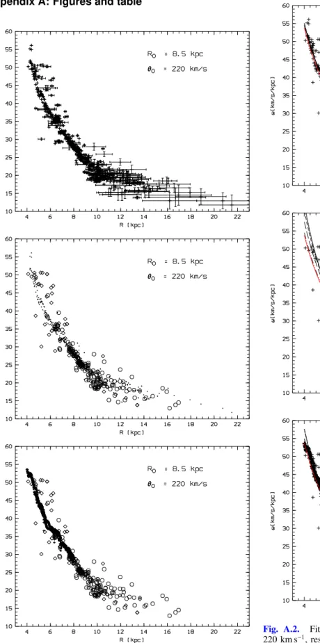
data, we checked the good agree-ment between them.

FigureA.1shows the different sub-samples and the typical error bars. By default, the tangent method always gives very small error bars and smaller scattering with respect to the H

_ii

regions and masers. In parallel, the galactocentric range around 8.5 kpc is naturally well populated by H

_ii

regions because at larger distance from the Sun the extinction no longer allows stel-lar distance determination. In the R ∼ 6 kpc to 8 kpc the tangent method data points and H

_ii

regions agree, while below 6 kpc, the masers show a clear offset from them.

In the literature, several expressions for the rotation curve are used:

– A polynomial form: θ(R)/ θ0 = a1 + a2r+ a3r2 with r =

((R/R0) − 1) used byReid et al.(2014).

– Power law forms: Honma et al. (2012) and Brand & Blitz (1993) used the following power law forms θ(R)/ θ0 = a1

(R/R0)a2and θ(R)/ θ0= a1(R/R0)a2+ a3, respectively.

– A universal form:Persic et al.(1996) suggest a more univer-sal form (θ(R)/θ0 = a1 [1+ a2 ((R/a3) − 1)])) based on a

sample of extragalactic rotation curves.

– The Polyex model:Giovanelli & Haynes (2002) used, to fit rotation curves for 2246 galaxies, another universal analyti-cal expression (known as the “polyex” model) with the form θ(R)/θ0= (1 − e−R/a1) × (1+ (a2R/a1)).

Before performing the fit we scale the data to the chosen R0,

θ0 set, following, for example, Xin & Zheng (2013). To

com-pare with the old and new results, we performed the fit on the three sub-samples with both R0 = 8.5 kpc, θ0 = 220 km s−1

and R0 = 8.34 kpc, θ0 = 240 km s−1 sets. In practice,

follow-ing Fich et al. (1989), the rotation curves are fitted in ω ver-sus R, because they are observationally independent quantities. We requested also that the cataloged objects have |b| < 3◦

(ob-jects with larger latitude are probably close ob(ob-jects for which the systemic velocity can be distorted by local motions) and L5, page 2 of7

(4)

R > 4 kpc because closer to the Galactic center the contribu-tion of the bulge and the bar to the kinematics can become im-portant (e.g.Chemin et al. 2015;Reid et al. 2014). The fits are done minimizing the normalised weighted χ2_{expression (where}

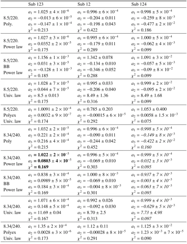
the weight is the inverse of the squared uncertainty) using the “Minuit” subroutine (Nelder & Mead 1965). The different fitted solutions are shown in Figs. A.2andA.3for the both adopted R0, θ0 sets, while the results are listed in TableA.1. Whatever

the model, the value of the standard normalised χ2 _{we found is}

small (between 0.09 and 0.45) while it is expected around unity. A value less than one does not necessary indicate a better fit but underlines uncertainty in the determination of the variance (Bevington & Robinson 2003). Despite the fact that it gives indi-cation about the data dispersion around the fited curve,Fich et al. (1989) show that the χ2numerical value cannot be easily used to sort the goodness of fit analysis. We then also used the evalu-ated parameter uncertainties3 to compare the fits because they are related to the width of the minimized expression minimum.

Looking at the figures we note the all the fitted curves give similar results except the polynomial form which, for several configurations, departs from the others after R = 8 kpc. From “Sub12”, we note also that all the models fit well the data in the range 6 to 10 kpc, while below 6 kpc they are not able to fit the regions offset from the tangent data. This underlines the fact that adding the tangent data will not impact too much the fitted curve in such inner parts and that fixing R0, θ0strongly forces the fit in

this distance range.

5. Discussion

To compare our results with previous studies we have to keep in mind that we fit with fixed R0 and θ0, as did

McClure-Griffiths & Dickey (2016) and Levine et al. (2008), for example, whileReid et al.(2014) andHonma et al.(2012), for example, have them as free parameters. In addition, Reid & Dame(2016) found that a slightly curved rotation curve with θ0 = 240 km s−1 can mimic a flat rotation curve with

θ0= 220 km s−1, convincing us to fit with fixed R0and θ0.

How-ever fixing R0and θ0implies some expected relation between the

fitted parameters. For example, a1 ∼ 1 is expected for Polyno-mial and Power-law models while a3 and a1 close to R0is

ex-pected for the Universal and Polyex models, respectively. Any large departure from these expected values underlines a least good fit, however, for most of the fitted parameters and the ex-pected values are in agreement.

A possible approach followed by several authors to study the rotation curve is to simply fit a linear expression of the form θ(R)/θ0 = a1 + a2 (R/R0). Some authors fit only the inner part

of the rotation curve (3 to 8 kpc), because this is traced from the tangent velocity method. This is the case for Fich et al.(1989) for quadrant I,Levine et al.(2008) for quadrants I and IV and McClure-Griffiths & Dickey(2016) for quadrant I, who find (a1,

a2)= (0.887,0.186), (0.855,0.024), (0.829,0.026), (0.82,0.026),

respectively. Others fit a linear rotation curve to data within 4 and 16 kpc (Reid et al. 2014) or even within 8 and 11 kpc (Huang et al. 2016) finding (a1, a2)= (1.007, −8.3 × 10−3) and

(1.23, −0.023), respectively. We note that focussing on the inner rotation curve gives a positive slope while fitting up to a larger radius changes the slope to negative (but close to zero value).

We first test the polynomial model. In this model a1 ×θ0

gives the overall amplitude of the rotation curve, and a2and a3 3 _{See the Minuit reference manual at} _{https://root.cern.ch/} sites/d35c7d8c.web.cern.ch/files/minuit.pdf

describe the position of the curve extremum (with respect to R0)

and the curve inflection, respectively. For a decreasing curve, a3

must be negative while the smaller|a3| is, the flatter the curve.

Reid et al.(2014), fitting such a form to masers, found a1, a2,

a3 = 1, 0.002, −0.06 (following our parameter definitions).

Fo-cussing on the two curves of “Sub12”, we find a similar a1 but

a systematically larger|a3| suggesting our curves are more

de-creasing. However, we can note that the polynomial form con-sistently gives the worst χ2 _{with respect to the other forms as}

can also be seen in Figs.A.2andA.3.

In the “polyex” expression,Giovanelli & Haynes(2002) de-scribe a1 as the scale length for the inner steep rise (the

ra-dial distance at which θ is 0.63 of the asymptotic velocity for a flat rotation curve) while a2 sets the slope of the

rota-tion curve’s outer part. From approximately 2200 low-redsift galaxies, Catinella et al. (2006) show that 0.002 < a2 <

0.087. However, for galaxies with maximum velocity around 220−240 km s−1_{, a}

2 is expected to be between approximately

0.003 and 0.006. Similar values are found for “Sub 123” and “Sub 124” while for “Sub 12” it is found negative but still close to zero. InCatinella et al.(2006), a1 is in units of exponential

disk scale length (Rd) and for galaxies with maximum

veloc-ity around 220−240 km s−1, it is estimated around 0.45. With a disk scale length for our Galaxy between 2.15 kpc (Bovy & Rix 2013) and 3.19 kpc (Sofue 2012) we expect a1 to be between

1.07 and 1.43 kpc. But whatever our sample, a1is found around

1 kpc and even smaller for “Sub 12” (with the IAU R0, θ0).

In the Universal law expression, a1 ×θ0 is the maximum

velocity, a3 is the radius where this maximum velocity (also

noted Rmax) is reached and a2is the velocity variation between

a3 and Ropt. As expected, a1 is close to 1 whatever the sample.

Persic et al.(1996) find −0.1 ≤ a2≤ 0.6. We find such values for

all our fitting configurations. FromPersic et al.(1996), usually a3 ∼ 2.2 × Rd, which suggest a3between 4.7 kpc and 7 kpc for

our Galaxy. For R0 = 8.5 kpc, a3is found very close to R0while

for R0 = 8.34 kpc a departure is noted reaching 40% for “Sub

123”.Reid et al.(2014) also fit such a Universal law to masers and find a1, a2, a3 = 1, 0.003, 12.13 kpc (following our

parame-ter definitions and with their R0, θ0 = 8.31 kpc and 241 km s−1)

which suggests a flatter rotation curve.

In the power law forms, a2, the exponent, describes how

quickly the curve decreases/increases while a3 is the deviation

term, which represents a simple way for observations to devi-ate from the power-law function. We note that a1 + a3 ∼ 1,

as expected for the Brand & Blitz(1993) form, is well recov-ered for IAU R0, θ0 while it is slightly smaller for R0, θ0 =

8.34 kpc and 240 km s−1. In addition to their H

_ii

regions cat-alog,Brand & Blitz(1993) added H

_i

tangent velocities to com-pute a rotation curve (with R0, θ0= 8.5 kpc, 220 km s−1) with the

power law form and found a1, a2, a3= 1.00767, 0.0394, 0.00712

similar to our results obtained for “Sub 123” and “Sub 124”.

6. Conclusion

Testing different analytical forms to different samples we find that all the forms, except the polynomial one, give satisfactory fitting results. The two power-law forms are often superimposed. The models used in extra-galactic studies (universal and polyex forms) are also tested. However they implement a radius scaling parameter which is difficult to relate to R0as is the case for the

other form. Using a stellar/maser distance sample gives more de-partures, even if the fits are good, between the different forms; in particular in the outer part of the rotation curve. In addition,

(5)

A&A 601, L5 (2017)

in the inner part, the fitted curve is not able to pass through the data points but passes at the expected location of the tangent point as plotted by “Sub 123” and “Sub 124”. The power-law appears then as the simplest and easiest form describing the ro-tation curve, and because the two power forms are often super-imposed, we favour the simplest form (with no a3). In the frame

of the kinematic distance determination of the Hi-GAL sources, we then adopt the power law form θ(R)/θ0 = 1.022 (R/R0)0.0803

with R0, θ0= 8.34 kpc, 240 km s−1.

To improve the Galactic rotation curve it appears important to better sample its outer part (R > 10 kpc). In this framework, we expect that the incoming ESA-Gaia database and maser parallactic distances will provide such information. Indeed, the ESA-Gaia database should provide better distance and rotation velocity determination (and velocity field) for the OB stars excit-ing the H

_ii

regions and identify and quantify the circular veloc-ity departures of such regions (in the detection limits). It will also allow one to trace the galactic rotation curve (and the velocity field) given by the stellar background potential and to compare it to the observed one, as it is expected (Gómez 2006) that the ob-served rotation curve is systematically above the true one. Maser parallax distances appear also as a very accurate and promising tool (and complementary to Gaia) for directly determining the distance of the star-forming regions in which Hi-GAL sources are located.

Acknowledgements. This work is part of the VIALACTEA Project, a Collabo-rative Project under Framework Programme 7 of the European Union, funded under Contract # 607380 that is hereby acknowledged.

References

Bevington, P. R., & Robinson, D. K. 2003, Data reduction and error analysis for the physical sciences (McGraw-Hill)

Blitz, L., & Spergel, D. N. 1991,ApJ, 370, 205

Blitz, L., Fich, M., & Stark, A. A. 1982,ApJS, 49, 183

Bobylev, V. V. 2017, Astron. Lett., in press, ArXiv e-prints [arXiv:1611.01766]

Boehle, A., Ghez, A. M., Schödel, R., et al. 2016,ApJ, 830, 17

Bovy, J., & Rix, H.-W. 2013,ApJ, 779, 115

Brand, J., & Blitz, L. 1993,A&A, 275, 67

Burton, W. B., & Gordon, M. A. 1978,A&A, 63, 7

Catinella, B., Giovanelli, R., & Haynes, M. P. 2006,ApJ, 640, 751

Chatzopoulos, S., Fritz, T. K., Gerhard, O., et al. 2015,MNRAS, 447, 948

Chemin, L., Renaud, F., & Soubiran, C. 2015,A&A, 578, A14

Clemens, D. P. 1985,ApJ, 295, 422

Feast, M., & Whitelock, P. 1997,MNRAS, 291, 683

Fich, M., Blitz, L., & Stark, A. A. 1989,ApJ, 342, 272

Georgelin, Y. M., & Georgelin, Y. P. 1976,A&A, 49, 57

Gillessen, S., Eisenhauer, F., Fritz, T. K., et al. 2013, in Advancing the Physics of Cosmic Distances, ed. R. de Grijs,IAU Symp., 289, 29

Giovanelli, R., & Haynes, M. P. 2002,ApJ, 571, L107

Gómez, G. C. 2006,AJ, 132, 2376

Honma, M., & Sofue, Y. 1997a,PASJ, 49, 539

Honma, M., & Sofue, Y. 1997b,PASJ, 49, 453

Honma, M., Nagayama, T., Ando, K., et al. 2012,PASJ, 64, 136

Hou, L. G., & Han, J. L. 2014,A&A, 569, A125

Huang, Y., Liu, X.-W., Yuan, H.-B., et al. 2016,MNRAS, 463, 2623

Kerr, F. J. 1964, in The Galaxy and the Magellanic Clouds, ed. F. J. Kerr,IAU Symp., 20, 81

Levine, E. S., Heiles, C., & Blitz, L. 2008,ApJ, 679, 1288

McClure-Griffiths, N. M., & Dickey, J. M. 2007,ApJ, 671, 427

McClure-Griffiths, N. M., & Dickey, J. M. 2016,ApJ, 831, 124

McClure-Griffiths, N. M., Dickey, J. M., Gaensler, B. M., et al. 2005,ApJS, 158, 178

Meyer, L., Ghez, A. M., Schödel, R., et al. 2012,Science, 338, 84

Molinari, S., Schisano, E., Elia, D., et al. 2016,A&A, 591, A149

Molinaro, M., Butora, R., Bandieramonte, M., et al. 2016,Proc. SPIE, 9913, 99130H

Nelder, J., & Mead, R. 1965,Comput. J., 7, 308

Persic, M., Salucci, P., & Stel, F. 1996,MNRAS, 281, 27

Pilbratt, G. L., Riedinger, J. R., Passvogel, T., et al. 2010,A&A, 518, L1

Reid, M. J., & Brunthaler, A. 2004,ApJ, 616, 872

Reid, M. J., & Dame, T. M. 2016,ApJ, 832, 159

Reid, M. J., Menten, K. M., Zheng, X. W., et al. 2009,ApJ, 700, 137

Reid, M. J., Menten, K. M., Brunthaler, A., et al. 2014,ApJ, 783, 130

Sofue, Y. 2012,PASJ, 64, 75

Sofue, Y., Honma, M., & Omodaka, T. 2009,PASJ, 61, 227

Stil, J. M., Taylor, A. R., Dickey, J. M., et al. 2006,AJ, 132, 1158

Xin, X.-S., & Zheng, X.-W. 2013,Res. Astron. Astrophys., 13, 849

(6)

Appendix A: Figures and table

Fig. A.1. Data sample used for the rotation curve fitting. The upper

panelshows the error bars. The middle panel shows sources from sam-ple 1 (circles), samsam-ple 2 (diamonds), and samsam-ple 3 (dots), respectively. The lower panel shows sample 4 (dots) instead of sample 3 while the other symbols are similar as in middle panel.

Fig. A.2. Fitted rotation curves with R0, θ0 set to 8.5 kpc and

220 km s−1_{, respectively. The fitted}_{Brand & Blitz}₍₁₉₉₃_{), power law,}

polynomial, Universal and polyex forms are displayed as solid, dot-ted, long dash, short dash, and dash-dot lines, respectively. The

(7)

A&A 601, L5 (2017)

Fig. A.3. As in Fig.A.2but for R0, θ0set to 8.34 kpc and 240 km s−1

re-spectively. TheReid et al.(2014) polynomial (long dashes), power-law (dotted line) and universal (short dashes) rotation curves are superim-posed (in red).

(8)

Table A.1. Fitting results.

Sub 123 Sub 12 Sub 124

8.5/220. Poly. a1= 1.025 ± 4 × 10−6 a2= −0.013 ± 6 × 10−5 a3= −0.147 ± 1 × 10−4 χ2_{= 0.213} a1= 0.996 ± 6 × 10−4 a2= −0.204 ± 0.011 a3= −0.198 ± 0.043 χ2_{= 0.422} a1= 0.998 ± 5 × 10−4 a2= −0.259 ± 8 × 10−3 a3= −0.477 ± 2 × 10−2 χ2_{= 0.186} 8.5/220. Power law a1= 1.027 ± 3 × 10−6 a2= 0.0352 ± 2 × 10−5 χ2_{= 0.175} a1= 0.995 ± 6 × 10−4 a2= −0.179 ± 0.011 χ2_{= 0.289} a1= 1.000 ± 5 × 10−4 a2= −0.062 ± 4 × 10−3 χ2_{= 0.099} 8.5/220. BB Power law a1= 1.156 ± 1 × 10−3 a2= 0.031 ± 3 × 10−5 a3= −0.128 ± 1 × 10−3 χ2_{= 0.185} a1= 1.342 ± 0.078 a2= −0.134 ± 0.010 a3= −0.346 ± 0.052 χ2_{= 0.288} a1= 1.091 ± 3 × 10−2 a2= −0.057 ± 5 × 10−3 a3= −0.09 ± 8 × 10−2 χ2_{= 0.099} 8.5/220. Univ. law a1= 1.028 ± 7 × 10−5 a2= 0.044 ± 7 × 10−5 a3= 8.5 ± 0.013 χ2_{= 0.175} a1= 0.995 ± 0.033 a2= −0.206 ± 0.040 a3= 8.49 ± 1.36 χ2_{= 0.316} a1= 0.999 ± 2 × 10−2 a2= −0.095 ± 2 × 10−2 a3= 8.49 ± 1.68 χ2_{= 0.099} 8.5/220. Polyex Univ. law a1= 1.0091 ± 2 × 10−4 a2= 0.0032 ± 9 × 10−7 χ2_{= 0.174} a1= 0.785 ± 0.203 a2= −0.00015 ± 6 × 10−5 χ2_{= 0.292} a1= 1.053 ± 0.400 a2= 0.0058 ± 1.5 × 10−3 χ2_{= 0.075} 8.34/240. Poly a1= 1.032 ± 2 × 10−5 a2= 0.221 ± 2 × 10−4 a3= 0.216 ± 4 × 10−4 χ2_{= 0.215} a1= 0.996 ± 6 × 10−4 a2= −0.090 ± 0.011 a3= −0.244 ± 0.042 χ2_{= 0.452} a1= 0.998 ± 5 × 10−4 a2= −0.149 ± 8 × 10−3 a3= −0.422 ± 2 × 10−2 χ2_{= 0.160} 8.34/240. Power law a1= 1.022 ± 2 × 10−5 a2= 0.0803 ± 4 × 10−5 χ2_{= 0.169} a1= 0.996 ± 5 × 10−4 a2= −0.069 ± 0.010 χ2_{= 0.303} a1= 0.999 ± 5 × 10−4 a2= 0.032 ± 3 × 10−3 χ2_{= 0.095} 8.34/240. BB Power law a1= 0.838 ± 3 × 10−4 a2= 0.0989 ± 5 × 10−5 a3= 0.184 ± 3 × 10−4 χ2_{= 0.169} a1= 1.000 ± 8 × 10−3 a2= −0.069 ± 0.010 a3= −0.004 ± 8 × 10−3 χ2_{= 0.301} a1= 0.937 ± 7 × 10−3 a2= 0.003 ± 4 × 10−3 a3= 0.063 ± 7 × 10−3 χ2_{= 0.095} 8.34/240. Univ. law a1= 1.071 ± 6 × 10−4 a2= 0.148 ± 5 × 10−4 a3= 11.69 ± 0.04 χ2_{= 0.167} a1= 0.992 ± 0.026 a2= −0.092 ± 0.030 a3= 8.70 ± 2.5 χ2_{= 0.313} a1= 0.999 ± 4 × 10−3 a2= −0.629 ± 5 × 10−3 a3= 7.73 ± 4.98 χ2_{= 0.097} 8.34/240. Polyex Univ. law a1= 1.35 ± 2 × 10−4 a2= 0.0028 ± 3 × 10−6 χ2_{= 0.173} a1= 1.12 ± 0.11 a2= −0.00028 ± 8 × 10−5 χ2_{= 0.291} a1= 1.125 ± 3 × 10−2 a2= 1.23 × 10−3± 7 × 10−5 χ2_{= 0.090}