HAL Id: insu-01802135
https://hal-insu.archives-ouvertes.fr/insu-01802135
Submitted on 7 Nov 2020
HAL is a multi-disciplinary open access
archive for the deposit and dissemination of
sci-entific research documents, whether they are
pub-lished or not. The documents may come from
teaching and research institutions in France or
abroad, or from public or private research centers.
L’archive ouverte pluridisciplinaire HAL, est
destinée au dépôt et à la diffusion de documents
scientifiques de niveau recherche, publiés ou non,
émanant des établissements d’enseignement et de
recherche français ou étrangers, des laboratoires
publics ou privés.
multi-variable dataset and application to the SIRTA
supersite
Marjolaine Chiriaco, Jean-Charles Dupont, Sophie Bastin, Jordi Badosa, Julio
López, Martial Haeffelin, Hélène Chepfer, Rodrigo Guzman
To cite this version:
Marjolaine Chiriaco, Jean-Charles Dupont, Sophie Bastin, Jordi Badosa, Julio López, et al.. ReOBS:
a new approach to synthesize long-term multi-variable dataset and application to the SIRTA supersite.
Earth System Science Data, Copernicus Publications, 2018, 10 (2), pp.919 - 940.
�10.5194/essd-10-919-2018�. �insu-01802135�
https://doi.org/10.5194/essd-10-919-2018 © Author(s) 2018. This work is distributed under the Creative Commons Attribution 4.0 License.
ReOBS: a new approach to synthesize long-term
multi-variable dataset and application to
the SIRTA supersite
Marjolaine Chiriaco1, Jean-Charles Dupont2, Sophie Bastin1, Jordi Badosa4, Julio Lopez2, Martial Haeffelin2, Helene Chepfer3, and Rodrigo Guzman3
1LATMOS/IPSL, UVSQ Université Paris-Saclay, UPMC Univ. Paris 06, CNRS, Guyancourt, France 2Institute Pierre Simon Laplace, Ecole Polytechnique, Université Paris-Saclay, Palaiseau, France
3Laboratoire de Météorologie Dynamique, Univ. Pierre and Marie Curie, Paris, France 4Laboratoire de Météorologie Dynamique, Ecole Polytechnique, Palaiseau, France
Correspondence:Marjolaine Chiriaco ([email protected])
Received: 6 September 2017 – Discussion started: 10 January 2018 Revised: 4 April 2018 – Accepted: 17 April 2018 – Published: 23 May 2018
Abstract. A scientific approach is presented to aggregate and harmonize a set of 60 geophysical variables at hourly timescale over a decade, and to allow multiannual and multi-variable studies combining atmospheric dynamics and thermodynamics, radiation, clouds and aerosols from ground-based observations. Many datasets from ground-based observations are currently in use worldwide. They are very valuable because they contain complete and precise information due to their spatio-temporal co-localization over more than a decade. These datasets, in particular the synergy between different type of observations, are under-used because of their com-plexity and diversity due to calibration, quality control, treatment, format, temporal averaging, metadata, etc. Two main results are presented in this article: (1) a set of methods available for the community to robustly and reliably process ground-based data at an hourly timescale over a decade is described and (2) a single netCDF file is provided based on the SIRTA supersite observations. This file contains approximately 60 geophysical variables (atmospheric and in ground) hourly averaged over a decade for the longest variables. The netCDF file is available and easy to use for the community. In this article, observations are “re-analyzed”. The pre-fix “re” refers to six main steps: calibration, quality control, treatment, hourly averaging, homogenization of the formats and associated metadata, as well as expertise on more than a decade of observations. In contrast, previous studies (i) took only some of these six steps into account for each variable, (ii) did not aggregate all variables together in a single file and (iii) did not offer an hourly resolution for about 60 variables over a decade (for the longest variables). The approach described in this article can be applied to different supersites and to additional variables. The main implication of this work is that complex atmospheric observations are made read-ily available for scientists who are non-experts in measurements. The dataset from SIRTA observations can be downloaded at http://sirta.ipsl.fr/reobs.html (last access: April 2017) (Downloads tab, no password required) under https://doi.org/10.14768/4F63BAD4-E6AF-4101-AD5A-61D4A34620DE.
1 Introduction
The Intergovernmental Panel on Climate Change (IPCC) simulations show a large spread between models when pre-dicting future climate at a global scale, but also when rep-resenting the observed current climate. These model uncer-tainties are larger at the regional scale and at short timescales (e.g., seasonal scale). These scales are, however, key for the impact assessment. For example, models do not reproduce observed magnitudes of interannual and seasonal variability and extremes in temperature and precipitation (Terray and Boé, 2013). Hawkins and Sutton (2009) also show that cli-mate’s natural variability is the main source of uncertainty to predict regional climate evolution at the timescale of 10– 20 years (compared to the selected scenario or model). Ob-servations of the atmosphere must be considered in order to improve both our knowledge of the processes that create this temporal variability and the simulation uncertainties. These observations must describe atmospheric processes that in-volve a large number of variables in the atmospheric columns and in the ground, and at various spatial and temporal scales. Multiannual and multi-variable datasets are therefore nec-essary. Many of these datasets from ground-based observa-tions have a significant scientific value because they con-tain complete and precise information on one or several decades, due to their spatio-temporal co-localization. Super-site observatories such as the Site Instrumental de Recherche par Télédétection Atmosphérqiue (SIRTA, Haeffelin et al., 2005) or the different Atmospheric Radiation Measurements (ARM, Ackerman et al., 2003) are among these sets of servations. But they are under-used, in particular the ob-served synergy aspects, because of their complexity and diversity in terms of calibration procedures, quality con-trol, data treatment, file format, temporal representativeness, metadata etc., and because of the weak magnitude of the sig-nals to be highlighted (e.g., trend versus natural variability), and also because of the complex connections between local-scale processes and climatic-local-scale anomalies (e.g., links between ground–boundary-layer–atmosphere processes and heat waves; as in Chiriaco et al., 2014).
An important homogenization work was needed for these observations. Homogenization has been performed for ARM observatories leading to the ARMBE (ARM Best Estimate) data product (Xie et al., 2010), which is the “ARM data streams specifically tailored to climate modelers for use in the evaluation of global climate models. They contain a best estimate of several cloud, radiation and atmospheric quan-tities. The ARMBE dataset was created to showcase all the flagship products of ARM” (from https://www.arm.gov/ capabilities/vaps/armbe, last access: April 2017). A speci-ficity of ARMBE products is that all variables are gath-ered in only two files: ARMBEATM (ATM for atmosphere) for many atmospheric state profiles and surface quantities, and ARMBECLDRAD (CLDRAD for cloud and radiation)
that contains a best estimate of several selected ARM and satellite-measured cloud- and radiation-relevant quantities.
In this article, additional steps are applied to the obser-vations and precisely described in order to understand how the observations are “re-analyzed”. This method is called ReOBS. The prefix “Re” refers to six main steps on more than a decade of observations: calibration, quality control, algorithmic treatment, hourly averaging, homogenization of the data formats and associated metadata, as well as scien-tist expertise. In contrast, previous studies (i) only take into account some of these six steps for each variable, (ii) do not aggregate together all variables in a single file and (iii) do not offer an hourly resolution for about 60 variables over a decade (for the oldest variables).
The ReOBS method was initially inspired by the ARMBE project and has been developed at SIRTA (located 20 km southwest of Paris, France). The SIRTA observatory has been collecting data for 15 years from active and passive remote sensing, in situ measurements at the surface, in the ground and in the planetary boundary layer (PBL). Early versions of the SIRTA ReOBS dataset have already been used in scientific studies that required the multi-variables and multi-temporal scales available in the SIRTA-ReOBS dataset (Cheruy et al., 2012; Chiriaco et al., 2014; Pal and Haeffelin, 2015, Bastin et al., 2016; Dione et al., 2017). The ReOBS method has also been tested for other supersites for some variables (classical meteorology, radiative fluxes, heat fluxes): Cabauw (in the Netherlands) and Chilbolton (in England) supersites in the framework of the EUCLIPSE European project (European Union Cloud Intercomparison, Process Study and Evaluation project), CO-PDD (Cézeaux – Opme – Puy De Dôme at Clermont Ferrand in France) and P2OA (Plateforme Pyrénéenne d’Observations Atmo-sphériques at Lannemezan in France) in Dione et al. (2016). The objective of the current paper is to present a scien-tific approach (ReOBS) to aggregate and harmonize about 60 geophysical variables at hourly timescale over at least a decade, and to study atmospheric dynamics and thermo-dynamics, radiation, clouds and aerosols from ground-based observations. This paper presents two main results: (1) a set of methods available for the community to process ground-based data robustly and reliably at an hourly timescale over at least a decade and (2) provision of a single netCDF file containing about 60 substantial geophysical variables hourly averaged over 15 years for the oldest ones, and easily usable for the community.
The SIRTA observations used for applying the ReOBS method are described in Sect. 2. The method used for Re-OBS is then detailed in Sect. 3. Section 4 presents the con-tents of the SIRTA-ReOBS file and its major strengths: the vertical profiles, the temporal scales and the multi-parameter specificity. Discussion and conclusions are pre-sented in Sect. 5.
2 Observations
2.1 SIRTA observatory
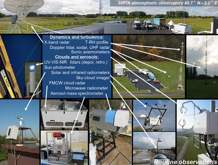
SIRTA is a French national observatory dedicated to the monitoring of tropospheric clouds and aerosols, the dynam-ics and thermodynamdynam-ics of the boundary layer, and the tur-bulent and organized transport of water and energy near the surface. The SIRTA observatory is a mid-latitude site (48.71◦N, 2.2◦E) located in a semi-urban area on the Saclay plateau 20 km southwest of Paris, and hosts active and pas-sive remote-sensing instruments since 2002 (Haeffelin et al., 2005). The SIRTA missions are (1) to monitor continuously and in the long-term the atmospheric column using a core ensemble of instruments; (2) to coordinate field campaigns in order to address specific scientific questions, such as pro-cesses related to water vapor and clouds, the ultraviolet radia-tion, or the aerosol physics and chemistry; and (3) to provide teaching resources and to host experimental training activi-ties.
Figure 1 shows a selection of SIRTA routine measure-ments from the different on-site locations (e.g., roof, mast, plain). The measurements used in the current study are listed in Table 1. Lidars play a special role in the SIRTA instru-mental park because several lidars have been deployed at the SIRTA observatory over the past 15 years, providing a unique 3-D database: (1) a dual-wavelength (532 and 1064 nm) de-polarization lidar (called LNA for “cloud and aerosol lidar”, used in the current study) from 2002 until 2015 (Haeffelin et al., 2005), (2) a multi-wavelength elastic (355, 532, 1064 nm) and Raman (387, 408, 607 nm) depolarization lidar (called IPRAL for “IPSL Hi-Performance multi-wavelength Raman Lidar for Cloud Aerosol Water Vapor Research”) since mid-2015, (3) an automatic 355 nm backscatter and depolariza-tion lidar (Leosphere ALS 450, used in this study) from 2008 until 2014 and (4) an automatic 1064 nm lidar ceilome-ter (Lufft CHM15k) since mid-2015. The different lidars differ significantly in complexity, emitted power, detection channels, signal-to-noise ratio and capacity to operate au-tonomously. For instance, the LNA backscattered signal pro-vides information on the presence of clouds and aerosols in the vertical column between 0.5 and 15 km altitude, whereas the ALS 450 backscatter lidar signal is exploited between 0.2 and 10 km.
2.2 SIRTA measurements used as inputs for ReOBS
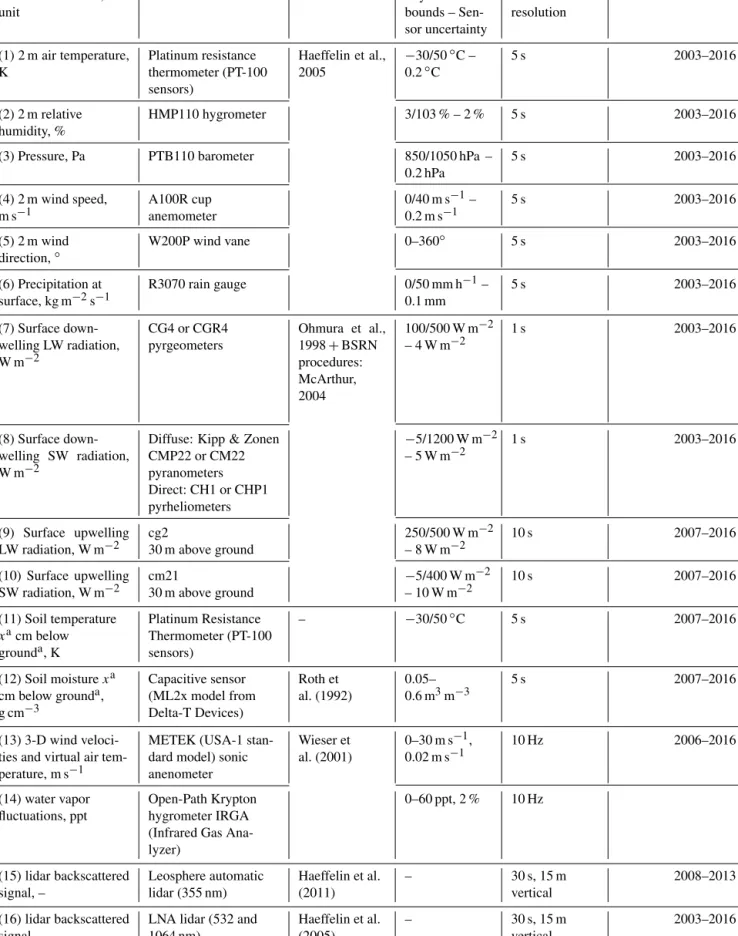
Table 1 shows the measurements used as inputs to create the SIRTA-ReOBS file. The table contains the instruments name, the physical bounds of the measurements, the native resolu-tion of the measurements and the available period of observa-tion. This set of variables includes in situ measurements (1–6 and 11–14 in Table 1), passive remote-sensing measurements (7–10 and 17–20) and active remote-sensing measurements (15–16 in Table 1).
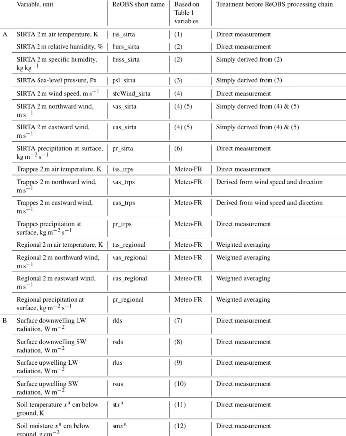
These different measurements are used to create the geo-physical variables listed in Table 2. Some of the geogeo-physical variables are directly measured, and some others require ad-vanced data processing, such as substantial quality control or algorithm application. Data processing performed inde-pendently of the ReOBS processing chain and already pub-lished is described and referenced in Table 2. The data pro-cessing developed in the framework of the ReOBS project is described in Sect. 3.
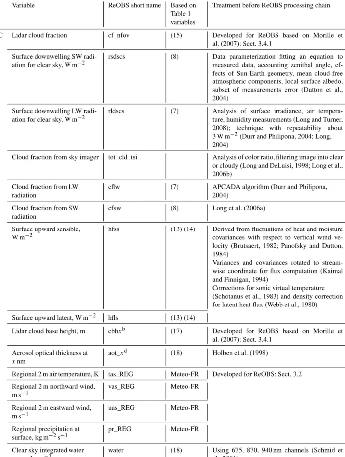
In the rest of the article, the geophysical variables are split into four groups. Group A contains the standard meteorol-ogy variables(first block in Table 2), such as 2 m tempera-ture, pressure, wind speed and direction, relative humidity, etc. Group B contains the advanced non-standard meteorol-ogy variables(second block in Table 2), such as radiative fluxes, heat fluxes, in-ground temperature and moisture, etc. These latter variables are directly measured but are usually not available from typical weather stations because they re-quire advanced technologies, for instance based on remote sensing. Group C contains variables retrieved from measure-mentsusing algorithms applied to remote-sensing measure-ments (third block in Table 2), such as cloud fraction, wa-ter vapor content, etc. Finally, group D contains atmospheric vertical profiles from lidar (fourth block in Table 2).
3 The ReOBS method
3.1 ReOBS general processing chain
The 15-year-long SIRTA-ReOBS dataset is contained in a single netCDF file containing hourly values of 63 physical variables listed in Table 2. The short and standard name used for each variable in the ReOBS dataset follows the Cou-pled Model Intercomparison Project (CMIP) and the Climate Forecast (CF) conventions, respectively, when available. For variables not included in CMIP or CF conventions, classical names are used or new ones are created.
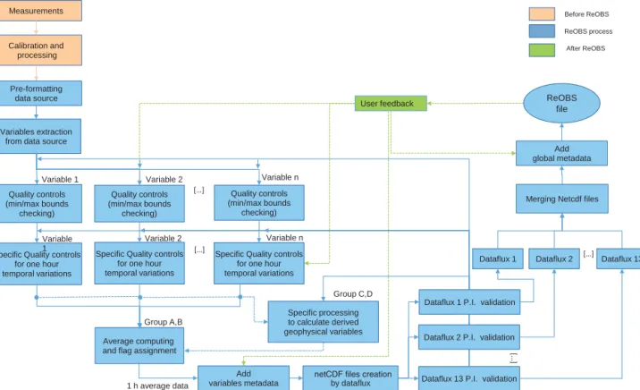
The strength of the ReOBS dataset is that all variables are processed using the same high-level processing chain, com-pleted by some sub-processing computations specific to each variable. Figure 2 shows the ReOBS processing chain (in blue in Fig. 2), which starts after the acquisition process (in orange in Fig. 2). Steps outside of the ReOBS processing chain are marked in green.
For each variable (except lidar profiles), the hourly mean values are calculated from the native resolution data (5 s to 1 min) by averaging all the data available within ±30 min around the full hour in order to be consistent with outputs from global circulation models (GCMs) and regional climate models (RCMs). Each hourly variable is completed by its intra-hour standard deviation. The hourly standard deviation (SD) of each variable helps in detecting non-physical spikes (i.e., successive increase and decrease) and dips (i.e., succes-sive decrease and increase in the signal). This temporal vari-ability information is also useful to document large changes
Figure 1.Photos of the routine instruments at the SIRTA supersite.
in the atmospheric conditions such as a cold front for air temperature, broken clouds for radiative fluxes and summer storms for precipitations or latent heat fluxes.
Variables entering the ReOBS dataset are quality-controlled at their native time resolution. The quality control test consists of verifying that the variable lies within physical bounds (Table 1). Calculations of hourly mean and standard deviation only use native resolution data that have passed quality control. A simple informative quality flag is associ-ated with each hourly value of a variable:
– 0: quality control is OK.
– 1: there are valid data but for less than 50 % of the period (that is, for less than 30 min).
– 2: flag 2 is only used for internal control and is never used as an informative output in the ReOBS file. – 3: data is unavailable for the entire hour (no
measure-ments or less than 50 % of the measuremeasure-ments in the hour
passes the quality control). In this case, the hourly value is set by convention to −999.96.
Besides the systematic quality tests described above, some additional complementary quality controls have been applied to specific variables, as described in the following subsec-tions (Sects. 3.2 to 3.5).
3.2 Specific computations for standard meteorological
variables
Classical meteorological variables collected at three differ-ent locations are included in the ReOBS dataset: (1) the first group of variables is collected at the SIRTA supersite and has the advantage of being representative of the very local meteorology since the beginning of the supersite activities, (2) the second group of variables aims at characterizing the surrounding meteorology around the SIRTA site and (3) the third group of variables is from the standardized Météo-France station, collected at Trappes, 15 km away from the SIRTA supersite. These three different datasets are identified
Table 1.List of variables measured at SIRTA and used as inputs for ReOBS. Measured variable,
unit
Instrument Reference Physical bounds – Sen-sor uncertainty Native resolution Period of observation (1) 2 m air temperature, K Platinum resistance thermometer (PT-100 sensors) Haeffelin et al., 2005 −30/50◦C – 0.2◦C 5 s 2003–2016 (2) 2 m relative humidity, % HMP110 hygrometer 3/103 % – 2 % 5 s 2003–2016
(3) Pressure, Pa PTB110 barometer 850/1050 hPa – 0.2 hPa 5 s 2003–2016 (4) 2 m wind speed, m s−1 A100R cup anemometer 0/40 m s−1– 0.2 m s−1 5 s 2003–2016 (5) 2 m wind direction,◦ W200P wind vane 0–360◦ 5 s 2003–2016 (6) Precipitation at surface, kg m−2s−1 R3070 rain gauge 0/50 mm h−1– 0.1 mm 5 s 2003–2016 (7) Surface down-welling LW radiation, W m−2 CG4 or CGR4 pyrgeometers Ohmura et al., 1998 + BSRN procedures: McArthur, 2004 100/500 W m−2 – 4 W m−2 1 s 2003–2016 (8) Surface down-welling SW radiation, W m−2
Diffuse: Kipp & Zonen CMP22 or CM22 pyranometers Direct: CH1 or CHP1 pyrheliometers −5/1200 W m−2 – 5 W m−2 1 s 2003–2016 (9) Surface upwelling LW radiation, W m−2 cg2 30 m above ground 250/500 W m−2 – 8 W m−2 10 s 2007–2016 (10) Surface upwelling SW radiation, W m−2 cm21 30 m above ground −5/400 W m−2 – 10 W m−2 10 s 2007–2016 (11) Soil temperature xacm below grounda, K Platinum Resistance Thermometer (PT-100 sensors) – −30/50◦C 5 s 2007–2016 (12) Soil moisture xa cm below grounda, g cm−3 Capacitive sensor (ML2x model from Delta-T Devices) Roth et al. (1992) 0.05– 0.6 m3m−3 5 s 2007–2016 (13) 3-D wind veloci-ties and virtual air tem-perature, m s−1
METEK (USA-1 stan-dard model) sonic anenometer Wieser et al. (2001) 0–30 m s−1, 0.02 m s−1 10 Hz 2006–2016 (14) water vapor fluctuations, ppt Open-Path Krypton hygrometer IRGA (Infrared Gas Ana-lyzer) 0–60 ppt, 2 % 10 Hz (15) lidar backscattered signal, – Leosphere automatic lidar (355 nm) Haeffelin et al. (2011) – 30 s, 15 m vertical 2008–2013 (16) lidar backscattered signal, –
LNA lidar (532 and 1064 nm) Haeffelin et al. (2005) – 30 s, 15 m vertical 2003–2016
Table 1.Continued. Measured variable, unity
Instrument Reference Physical bounds – Sen-sor uncertainty
Native resolution
Period of observation
(17) 360◦sky image, – Yankee Environmental System Total Sky Imager (TSI) Long et al. (1998) – 1 min 2009–2016 (18) 440–870 nm spectral irradiance
Cimel sunphotometer Dubovik et al. (2000)
– when sun disc is visible
2008–2016
(19) zenith path delay (ZPD), s
GPS Champolion et al. (2004)
– 15 min 2008–2016
(20) liquid water path RPG-HATPRO microwave radiometer
Rose et al. (2005)
– 1 s 2010–2016
axis 5, 10, 20, 30, 50 cm.
with the suffixes -sirta, -regional and -trps, respectively, in the following.
3.2.1 Description of surrounding meteorology around
the SIRTA site
Figure 3b–d illustrate the air temperature, wind speed, and cumulated precipitations probability density func-tions (PDFs) in relative occurrence at three Météo-France stations within a 50 × 50 km domain around the SIRTA su-persite: in Trappes (48.8◦N, 2.0◦W), in Paris-Montsouris (48.8◦N, 2.3◦W) and in Orly (48.7◦N 2.4◦W); these plots highlight the eventual differences from one site to another.
The PDF of the 2 m air temperature (noted tas in SIRTA-ReOBS) shows an offset of about 2◦C for the Paris-Montsouris site compared to the Orly, Trappes and SIRTA sites, which is due to the urban heat. Maximum values for the mean wind speed value (noted sfcWind in SIRTA-ReOBS) are measured at the Orly site and the mean wind speed is around 3 m s−1 at SIRTA. Note that measurements at the SIRTA site are performed over a roof: wind speed is thus measured at 10 m above the roof, corresponding to 25 m above ground level, whereas it is measured at 10 m above ground level for the other stations. Even if a ground level standard (Météo-France-like) meteorological station is also present at SIRTA, the rooftop measurements were preferred for the ReOBS file because they started earlier (in 2003) than the standard meteorological station (in 2006). The four sta-tions are characterized with a cumulated annual precipitation ranging between 600 and 700 mm yr−1.
The data collected at the three stations around the SIRTA supersite are used to characterize the surrounding 2 m mete-orology. A weight is assigned to each of the three stations based on the following method: the 50 km× 50 km domain is divided into 90 × 103grid boxes (300 × 300), the distance between each box and each site is calculated and then each
box is linked to its nearest site. Then the percentage number of boxes linked to each site gives the weight of the site within the domain. The weight of the Trappes station is then 44.4 %, the weight of the Orly station is 34.5 % and the weight of the Paris-Montsouris station is 21.1 % (Fig. 3a). The regional-scale meteorology variables v (−REG) included in ReOBS are then obtained from
¯ v = n X i xiwi, (1)
where x = {x1, . . ., x4}is the set of values taken by a variable
v(2 m temperature, humidity, wind, etc.) at each of the four stations, and w = {w1, . . ., w4}is the station weight.
3.2.2 Quality control of the standard meteorological
variables
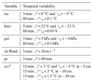
The quality control for meteorological variables listed in Ta-ble 2 consists of two additional tests compared to what was indicated in Sect. 3.1. The goal of the quality control is to reject unphysical values and to reject values with unrealis-tic temporal variability (Tables 1 and 3), e.g., non-physical jump in the data record, non-physical persistence in time of the measured values.
Non-physical jumps in the data are detected at native high temporal resolution (5 s). If the difference between two suc-cessive measurements is more than a specified limit given in Table 3 (these tests are about to be refined in a new study that will give a new version of the SIRTA-ReOBS file) the current measurement is rejected but it is used for checking the tem-poral consistency with the next measurement. Two examples of measurements that did not pass the quality control tests are shown in Fig. 4a and b for pressure and soil tempera-ture jumps, respectively. In the first example, an unphysical change of 2 hPa within 1 min is observed in pressure (larger than 5 hPa during 5 min, see Table 3). In the second example,
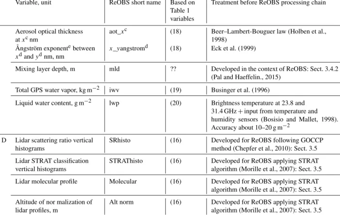
Table 2.Variables included in SIRTA-ReOBS. First block (category A) is for classical meteorological measurements, second block (cat-egory B) is for more advanced measurements, third block (cat(cat-egory C) is for parameters retrieved from observations and fourth block (category D) is for vertical lidar measurements.
Variable, unit ReOBS short name Based on Table 1 variables
Treatment before ReOBS processing chain
A SIRTA 2 m air temperature, K tas_sirta (1) Direct measurement SIRTA 2 m relative humidity, % hurs_sirta (2) Direct measurement SIRTA 2 m specific humidity,
kg kg−1
huss_sirta (2) Simply derived from (2)
SIRTA Sea-level pressure, Pa psl_sirta (3) Simply derived from (3) SIRTA 2 m wind speed, m s−1 sfcWind_sirta (4) Direct measurement SIRTA 2 m northward wind,
m s−1
vas_sirta (4) (5) Simply derived from (4) & (5)
SIRTA 2 m eastward wind, m s−1
uas_sirta (4) (5) Simply derived from (4) & (5)
SIRTA precipitation at surface, kg m−2s−1
pr_sirta (6) Direct measurement
Trappes 2 m air temperature, K tas_trps Meteo-FR Direct measurement Trappes 2 m northward wind,
m s−1
vas_trps Meteo-FR Derived from wind speed and direction
Trappes 2 m eastward wind, m s−1
uas_trps Meteo-FR Derived from wind speed and direction
Trappes precipitation at surface, kg m−2s−1
pr_trps Meteo-FR Direct measurement
Regional 2 m air temperature, K tas_regional Meteo-FR Weighted averaging Regional 2 m northward wind,
m s−1
vas_regional Meteo-FR Weighted averaging
Regional 2 m eastward wind, m s−1
uas_regional Meteo-FR Weighted averaging
Regional precipitation at surface, kg m−2s−1
pr_regional Meteo-FR Weighted averaging
B Surface downwelling LW radiation, W m−2 rlds (7) Direct measurement Surface downwelling SW radiation, W m−2 rsds (8) Direct measurement Surface upwelling LW radiation, W m−2
rlus (9) Direct measurement
Surface upwelling SW radiation, W m−2
rsus (10) Direct measurement
Soil temperature xacm below ground, K
stxa (11) Direct measurement
Soil moisture xacm below ground, g cm−3
Table 2.Continued.
Variable ReOBS short name Based on Table 1 variables
Treatment before ReOBS processing chain
C Lidar cloud fraction cf_nfov (15) Developed for ReOBS based on Morille et al. (2007): Sect. 3.4.1
Surface downwelling SW radi-ation for clear sky, W m−2
rsdscs (8) Data parameterization fitting an equation to measured data, accounting zenithal angle, ef-fects of Sun-Earth geometry, mean cloud-free atmospheric components, local surface albedo, subset of measurements error (Dutton et al., 2004)
Surface downwelling LW radi-ation for clear sky, W m−2
rldscs (7) Analysis of surface irradiance, air tempera-ture, humidity measurements (Long and Turner, 2008); technique with repeatability about 3 W m−2(Durr and Philipona, 2004; Long, 2004)
Cloud fraction from sky imager tot_cld_tsi Analysis of color ratio, filtering image into clear or cloudy (Long and DeLuisi, 1998; Long et al., 2006b)
Cloud fraction from LW radiation
cflw (7) APCADA algorithm (Durr and Philipona, 2004)
Cloud fraction from SW radiation
cfsw (8) Long et al. (2006a)
Surface upward sensible, W m−2
hfss (13) (14) Derived from fluctuations of heat and moisture covariances with respect to vertical wind ve-locity (Brutsaert, 1982; Panofsky and Dutton, 1984)
Variances and covariances rotated to stream-wise coordinate for flux computation (Kaimal and Finnigan, 1994)
Corrections for sonic virtual temperature (Schotanus et al., 1983) and density correction for latent heat flux (Webb et al., 1980) Surface upward latent, W m−2 hfls (13) (14)
Lidar cloud base height, m cbhxb (17) Developed for ReOBS based on Morille et al. (2007): Sect. 3.4.1
Aerosol optical thickness at xnm
aot_xd (18) Holben et al. (1998)
Regional 2 m air temperature, K tas_REG Meteo-FR Developed for ReOBS: Sect. 3.2 Regional 2 m northward wind,
m s−1
vas_REG Meteo-FR
Regional 2 m eastward wind, m s−1
uas_REG Meteo-FR
Regional precipitation at surface, kg m−2s−1
pr_REG Meteo-FR
Clear sky integrated water vapor, kg m−2
water (18) Using 675, 870, 940 nm channels (Schmid et al., 2001)
Table 2.Continued.
Variable, unit ReOBS short name Based on Table 1 variables
Treatment before ReOBS processing chain
Aerosol optical thickness at xcnm
aot_xc (18) Beer–Lambert-Bouguer law (Holben et al., 1998)
Ångström exponentebetween xdand ydnm, nm
x_yangstromd (18) Eck et al. (1999)
Mixing layer depth, m mld ?? Developed in the context of ReOBS: Sect. 3.4.2 (Pal and Haeffelin., 2015)
Total GPS water vapor, kg m−2 iwv (19) Businger et al. (1996)
Liquid water content, g m−2 lwp (20) Brightness temperature at 23.8 and 31.4 GHz + input from temperature and humidity sensors (Bosisio and Mallet, 1998). Accuracy about 10–20 g m−2
D Lidar scattering ratio vertical histograms
SRhisto (16) Developed for ReOBS following GOCCP method (Chepfer et al., 2010): Sect. 3.5 Lidar STRAT classification
vertical histograms
STRAThisto (16) Developed for ReOBS applying STRAT algorithm (Morille et al., 2007): Sect. 3.5 Lidar molecular profile Molecular (16) Developed for ReOBS applying STRAT
algorithm (Morille et al., 2007): Sect. 3.5 Altitude of nor malization of
lidar profiles, m
Alt norm (16) Developed for ReOBS applying STRAT algorithm (Morille et al., 2007): Sect. 3.5
axis 5, 10, 20, 30, 50 cm;
bxis first layer (1), second layer (2), third layer (3); cxis 1020, 870, 675, 500, 440, 380, 340 nm; dxand y are the interval betweencvalues.
enegative slope (or first derivative) of aerosol optical depth with wavelength in logarithmic scale is the Angstrom parameter (Eck et al., 1999, see Fig. 4r for
significance value).
several temperature spikes (0.6◦C within 1 min for ground at −5 cm) are detected and we reject the data when the increase reaches +3◦C and the decrease −4◦C within 15 min (i.e., +0.2 and −0.27◦C for 1 min resolution).
The unphysical persistence in time of the measured values are detected by verifying that the variability within 1 hour is physical, following values in Table 3. If the 1-minute val-ues do not vary by more than a specified lower limit (given in Table 3) within 1 hour, the current value fails the check. Figure 4d shows an example of an unphysical wind speed measured by a cup anemometer. The value is 0 m s−1 after 18:00 UT because of frost deposition on the sensor (shown by low temperature and high relative humidity in Fig. 4c). The persistence test is completed by a calculation of the stan-dard deviation of temperature, pressure, humidity and wind speed for the last 1-hour period. In combination with the per-sistence test, the evaluation of the standard deviation is a very good tool for the detection of a blocked sensor, as well as a 1 h sensor drift.
3.3 Specific computation for advanced meteorological
variables
The data quality of in-ground temperature and permeability of the soil is checked using the tests above (Table 1 and 3).
The quality of the downwelling shortwave (SW) and long-wave (LW) fluxes is tested following the recommendation of the Baseline Surface Radiation Network (BSRN; test version 2.0; Roesch et al., 2011). Additional semi-automatic controls were developed and applied to SW irradiances in order to reject data collected when the sun tracker failed (used for the direct and diffuse SW radiation measurements) and to re-move values that are inconsistent between measured global SW fluxes and global SW fluxes calculated from direct and diffuse measured ones. Individual 1 min native data not pass-ing the test are automatically removed before performpass-ing the 1 h averages. For SW fluxes, the global as well as the direct and diffuse irradiance components are included in the Re-OBS dataset. A best estimate of the global SW is calculated as a combination of the global irradiance measurement and the sum of the diffuse and horizontal direct irradiance
mea-Measurements
Calibration and processing
Variables extraction from data source
Specific Quality controls for one hour
temporal variations
Average computing and flag assignment
1 h average data
Specific processing to calculate derived geophysical variables
Dataflux 13 P.I. validation
netCDF files creation
by dataflux
Merging Netcdf files
Group C,D Group A,B ReOBS process Before ReOBS User feedback Pre-formatting data source Quality controls (min/max bounds checking) Quality controls (min/max bounds checking) Quality controls (min/max bounds checking)
Variable 1 Variable 2 Variable n
Specific Quality controls for one hour temporal variations
Specific Quality controls for one hour temporal variations
Add
variables metadata
Dataflux 13 Dataflux 1 Dataflux 2
Dataflux 1 P.I. validation
Dataflux 2 P.I. validation
ReOBS file Add global metadata […] […] Variable 1 Variable 2 Variable n […] […] After ReOBS
Figure 2.Schematic of the ReOBS general processing chain. Orange, blue, and green boxes and arrows are for steps before, during, and after, respectively, the ReOBS processing chain.
surements. The sum is taken as default and the blanks in ob-servations are filled with the global irradiance measurement. The sensible and latent heat flux data are subjected to spike detection and rejection algorithms. Sensible and latent heat fluxes are based on sonic measurements and a gas ana-lyzer. The lag between the sonic measurements and the gas analyzer is set to the lag of maximum correlation over the averaging interval between the sonic anemometer tempera-ture and the absolute humidity measured by the gas analyzer. At hourly intervals, sensible and latent heat fluxes are de-rived from eddy-covariance techniques, as well as turbulence statistics. Raw data and calculated statistics are subjected to strict data limits to reject unphysical values (13 and 14 in Table 1). For the latent heat flux, the open-path infrared gas analyzer (IRGA) used between 2005 and 2012 could be dam-aged by precipitations and was therefore manually switched on and off. The temporal sampling was thus relatively low and we decided to exchange the IRGA with an open-path LI-COR LI-7500 in 2012. With the open-path InfraRed Gas Analyser the molar density fluctuations are accounted for in the processing by following the classic formulation of Webb et al. (1980). Moreover, an automatic method has been ap-plied to correct wind statistics for any misalignment of the sonic anemometer with respect to the local wind stream-lines of the sonic anemometer with respect to the local wind streamlines according to Wilczak et al. (2001).
3.4 Retrievals based on remote-sensing measurements
developed for ReOBS
3.4.1 Computations for the cloud fraction and cloud
base height from lidar
The ReOBS dataset contains cloud base height and time se-ries of the cloud fraction (CF), deduced from the SIRTA 355 nm lidar and processed with the STRAT algorithm (STRucture of the ATmosphere; Morille et al., 2007). The cloud fraction (noted cf_nfov, where “nfov” stands for “nar-row field of view”) is defined as the number of profiles con-taining clouds divided by the total number of profiles col-lected in 1 hour. The cloud base height of the first layer (noted CBH1) corresponds to the altitude of the first cloud layer from the ground as detected by the STRAT algorithm. An hourly cloud base height is reported in ReOBS only if at least 33 % of the profiles collected during this hour are cloudy and only if less than 40 % of the profiles col-lected during this hour are noisy (i.e., at least 60 % of pro-files are valid). Sensitivity tests based on several case stud-ies have shown that taking less than this 33 % or more than this 40 % threshold leads to cloud base height values non-representative of what happens in the current hour. CBH2 and CBH3 are the altitudes of the base of a second and a third cloud layer, respectively, detected above CBH1 and
sep-Figure 3.(a) Location of the SIRTA supersite and the three neighboring Météo France stations with their associated weight as defined in the text. Relative occurrence of hourly mean air temperature (b) and wind speed (c) at SIRTA and at the neighboring Météo France stations between 2005 and 2014, and cumulated precipitation at SIRTA and at the neighboring Météo France stations in 2012 (d).
arated from the first cloud (the one with CBH1) with clear sky.
3.4.2 The mixing layer depth product
The mixing layer depth (MLD, noted mld in SIRTA-ReOBS) is part of the SIRTA-ReOBS database. It is retrieved from routine lidar measurements (ALS 450 from the Leosphere company) following the method described in Pal et al. (2013) and Haeffelin et al. (2012).
In this method, the intensity of the lidar-derived aerosol backscatter signal at different altitudes is used to determine the hourly-averaged vertical profiles of variance. Next, the location of maximum turbulent mixing within the mixing layer is determined and corresponds to the mean MLD. Micrometeorological measurements of the Monin–Obukhov length scale are used (effect of buoyancy on turbulent flow; Monin and Obukhov, 1954) to better determine the MLD, especially for the early morning transition and evening tran-sition periods. For these two specific periods, a first-order approximation of the boundary layer growth rates is ob-tained and the variance-based results guides the attribution by searching the minimum altitude of the gradient closest to the mean MLD. Two transition periods of a day are used to distinguish the turbulent regimes during the well-mixed
con-Table 3.Range of temporal variabilities considered when perform-ing the quality control for the variables listed in table. Upper arrows mean an increase during the time window indicated, and lower ar-rows mean a decrease during the time window indicated.
Variable Temporal variability
tas 5 min: % < 6◦C and & < −9◦C 60 min: %& > 0.1◦C
hurs 5 min: % < 22 % and & < −23 % 60 min: %& > 0.05 %
psl 5 min: % < 5 hPa and & < −4 hPa 60 min: %& > 0.1 hPa
sfcWind 5 min: % < 30 m s−1 pr 5 min: % < 40 mm
stxa 15 min: % < 3◦C and & < −4◦C at −5 cm 15 min: %& < 3◦C at −10 cm
15 min: %& < 1.5◦C at −30 cm 60 min: %& > 0.05◦C
axis 5, 10, 20, 30, 50 cm.
vective ABL (atmospheric boundary layer) and nocturnal or stable MLD.
3.5 Computations for the lidar profiles
The SIRTA ReOBS dataset contains information on the de-tailed vertical description of the atmosphere since 2002 from the LNA instrument. A drawback of this instrument is that it requires human intervention and does not operate when it rains, which introduces gaps in the data record.
Two different hourly variables are included in the ReOBS dataset:
– One variable called STRAThisto, which contains the number of occurrences of clear sky, aerosols, clouds, invalid data and fully attenuated laser within 1 hour for each vertical level. The vertical resolution is 15 m up to 15 km and the layer type classification is based on the STRAT algorithm.
– One variable called SRhisto is a 2-D height-intensity number of occurrences accumulated during 1 hour, as defined in Chepfer et al. (2010). We use the lidar scat-tering ratio SR = ATB / ATBmol, where ATB is the total
attenuated backscatter lidar signal and ATBmol is the signal in clear-sky conditions. The vertical resolution is 15 m and the intensity axis contains 18 bins; −999 / −777 / −666 / 0 / 0.01 / 1.2 / 3 / 5 / 7 / 10 / 15 / 20 / 25 / 30 / 40 / 50 / 60 / 80. The value “−999“ indicates non-normalized noisy profiles, the value “−777” is for profiles that cannot be normalized due to the presence of a very low cloud, and the value “−666” is for invalid data. ATB profiles are normalized to a daily molecular profile based on radiosounding measurements launched every day 10 km away from the SIRTA supersite (at the Météo-France station in Trappes). The altitude of nor-malization of ATB (which must be clear sky) is deter-mined for each profile using the STRAT algorithm.
4 Results
4.1 Description of the ReOBS database content
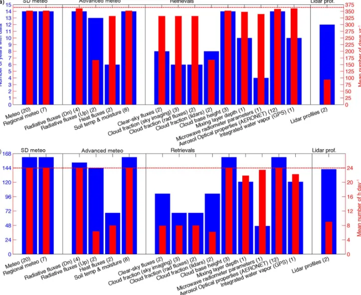
All data passing the quality control tests are included in the ReOBS final netCDF file. The variables included in the SIRTA-ReOBS are listed in Table 2 together with their nomenclature (Table 2, second column). There are 42 lines in Table 2, corresponding to 34 variables currently in the file. Figure 5 shows the temporal coverage of each variable. Some variables such as the classical meteorological variables or the downwelling radiative fluxes are very well sampled since 2002 when SIRTA activities started. In contrast, the record for lidar profiles, which started in 2002, contains many gaps. The sampling of the latent heat flux is much more intermit-tent than the sampling of the sensible heat flux due to instru-mental issues (see Sect. 3.3).
There are two versions of the SIRTA-ReOBS file: a com-plete file, which includes all information available (1.2 Gb),
and another one which contains all data except for the verti-cal information from the lidar (11.5 Mb): this last is signifi-cantly smaller and so it is easier to handle. Both data files are available on the following website: http://sirta.ipsl.fr/reobs. html (Downloads tab, no password required), which also in-cludes quicklooks and a documentation.
The main advantages of ReOBS compared to classical su-persite databases are (1) the vertical profile information com-ing from lidar measurements, which is user friendly thanks to the GOCCP (GCM Oriented CALIPSO Cloud Product) method (Chepfer et al., 2010), (2) the possibility to study the troposphere at different timescales (from daily to decadal timescales) and (3) the availability of a multi-variable syner-getic view of the atmosphere. And of course a mix of these three aspects. These three main added values are detailed in the following subsections.
4.2 Vertical profile information
The lidar profiles included in SIRTA-ReOBS provide use-ful information on the vertical distribution of clouds and aerosols in the atmosphere. This information together with many other SIRTA-ReOBS variables have been used recently in various studies (Cheruy et al., 2012; Chiriaco et al., 2014; Bastin et al., 2016). We first show examples of the two main ReOBS variables build from lidar measurements (SRhisto and STRAThisto) and we then describe how these data are used to built cloud fraction profiles. Finally, we describe how to use these data to evaluate clouds simulated by models.
4.2.1 SRhisto and STRAThisto
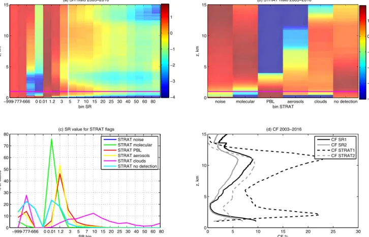
Figure 6 shows SRhisto (Fig. 6a) and STRAThisto (Fig. 6b) for every hour containing measurements from 2003 to 2016. Periods without lidar measurements are not included in this figure and this happens frequently (see Fig. 5) because mea-surements are only performed when it is not raining and with human intervention (i.e., not during night and weekends). Using SRhisto, the repartition of clouds can be analyzed as a function of altitude and as a function of the intensity of the lidar signal (SR), which is a proxy of the particle optical thickness. Fully attenuated lidar signals are located in the bin 0 < SR < 1, clear sky are found in the bin SR = 1, uncertain are in the bin 1 < SR < 5 (it could be aerosols for instance), and SR > 5 is for clouds (white vertical line in Fig. 6a; bins defined in Sect. 3.5). The analysis of SRhisto shows that non-precipitating clouds observed at SIRTA (note: the LNA lidar instrument does not operate when it rains) are mostly thin, low clouds (under 4 km with SR < 15) or thin, high clouds (above 7 km with SR < 20), and there are also thicker clouds with SR > 80 or fully attenuated lidar signal. There are al-most no mid-level clouds (between 4 and 7 km) and only few clouds with 20 < SR < 80. The analysis of STRAThisto indi-cates that for these non-precipitating cases, the amount of clouds that fully attenuates the lidar signal (i.e., “noise”) is
Figure 4.(a) Example of an unphysical jump in instantaneous values of pressure and (b) temperature in ground at 5 cm (black) and at 10 cm (red). (d) Example of unphysical persistence of high wind speed measurements using a cup anemometer due to frost in (c) (negative temperature in red and high humidity values in blue).
approximately on the same order of magnitude as the amount of thinner clouds.
Lidar profiles that would be measured in clear-sky con-ditions (so called molecular profiles) are necessary to build SRhisto and STRAThisto as it is used in the SR estimation and in the STRAT lidar profile normalization. These molec-ular profiles are estimated based on temperature and pres-sure profiles meapres-sured twice a day by METEO-FRANCE ra-diosounding at Trappes (10 km from SIRTA). These molec-ular lidar profiles are included in SIRTA-ReOBS under the Molecular variable, as well as the altitude of normalization used for STRAT under the Alt norm variable.
4.2.2 Cloud fraction profiles
Cloud fraction profiles are derived from the SRhisto or from the STRAThisto variables at a temporal scale ranging from 1 hour up to several years. At a given altitude level, the cloud fraction is the ratio between the occurrence of cloudy cases and the occurrence of all cases excluding the noisy ones. In STRAThisto the occurrence of cloudy layers is given in flag “clouds”. In SRhisto, a layer is declared cloudy in a lidar pro-file when SR > 5 and SR > 1+ε/ATBmolwith ε = 1.3 × 10⁻⁶
SI (ATBmol is included in SIRTA-ReOBS). As expected,
the cloud fraction profiles obtained from SRhisto or from STRAThisto (Fig. 6d) are different due to the differences in
the definition of the cloud detection in the two algorithms. In particular, SRhisto features less low-level clouds (z < 4 km) than STRAThisto. The magenta curve in Fig. 6c is the SR dis-tribution for cloudy cases during a given hour for the STRAT algorithm. This distribution shows that about 28 % of these cases correspond to cases where SR cannot be estimated be-cause of the presence of a very low cloud (−777 in Fig. 6c) preventing the normalization of the profile (no detection of molecular signal under the cloud). This could explain the differences in low cloud fractions between STRAThisto and SRhisto in Fig. 6d. The part of the magenta curve with val-ues of SR between 0.01 and 5 corresponds to cloudy cases for the STRAT algorithm but not based on the SR threshold method. This could explain the bias between CF SR and CF STRAT that occurs at almost all vertical levels. Red and yel-low curves in Fig. 6c also highlight the fact that most of the cases that are defined as PBL or aerosols for the STRAT al-gorithm are actually not cloudy when based on the SR thresh-old method (the parts of these curves above SR = 5 represent less than 5 %). The differences between STRAT- and SR-based algorithms illustrate the important sensitivity of the cloud fraction profile to the cloud definition. This sensitiv-ity needs to be taken into account when comparing the mea-surements to simulations from GCMs or RCMs in order to
Figure 5.Temporal coverage of groups of variables in the SIRTA-ReOBS dataset. In panel (a), blue bars indicate the total numbers of years with data and red bars indicate the mean numbers of days with measurements in a year. In panel (b), blue bars indicate the numbers of months with data and red bars indicate the mean numbers of hours with measurement in a day. The numbers in brackets are the number of variables in each sub-group. Variables are separated in four categories: classical meteorological measurements (group A, left), more advanced measurements (group B, center-left), variables retrieved from measurements (group C, center-right) and lidar profiles (group D, right). Dn means downward, Up means upward.
reproduce the algorithm hypotheses in the simulations; it is usually done using a lidar simulator described below.
4.2.3 Lidar simulator
For comparing the SIRTA-ReOBS SRhisto variable to GCM or RCM outputs, we have developed a ground-based lidar simulator, which is an adaptation of the CALIOP (Cloud-Aerosol Lidar with Orthogonal Polarization) lidar simulator (Chepfer et al., 2008), taking into account the specification due to the ground-based position of the instrument. In partic-ular, the vertical turnaround of the lidar equation following the very first version of lidar simulator described in Chiri-aco et al. (2006). Model outputs are used as inputs for the
lidar simulator to simulate what would be measured from the ground-based lidar if the atmosphere was the simulated one. First the lidar equation that gives the ATB as a function of altitude is used to simulate SR from model outputs. Then the same space and time resolutions as in observations and the SR thresholds are used for the simulated lidar profiles as in the actual data algorithm (SRhisto for SIRTA-ReOBS), making the lidar profiles directly comparable to the measured ones.
This ground-based version of the lidar simulator has been used for comparisons between the SIRTA-ReOBS lidar pro-files and the WRF/MED-CORDEX (Weather Research and Forecast model; Coordinated Regional Climate Downscaling
Figure 6.(a) Lidar scattering ratio (SR) histogram obtained by cumulating all SIRTA observation data from 2003 to 2016. The color bar is the logarithm of the percentage of occurrence (the sum of one line is equal to log(100 %)); the pink horizontal line corresponds to the altitude of recovery of the lidar (z = 1 km; below this altitude, lidar data is more complicated to use); the white vertical line corresponds to the threshold of cloud detection (SR = 5). (b) STRAT histogram obtained by cumulating all data from 2003 to 2016. The color bar is the logarithm of the percentage of occurrence. (c) Percentage of occurrence of SR values for the different STRAT flags (noise in blue – no cases actually –, molecular in green, PBL in red, aerosols in yellow, clouds in magenta and no detection in cyan), cumulating all altitudes above 1 km and only for hours containing a single STRAT flag. (d) Fraction of clouds (in %): CF SR1 (black solid line) is the occurrence of SR > 5 versus the occurrence of SR > 0, CF SR2 (gray solid line) is the occurrence of SR > 5 vs. the total occurrence of profiles, CF STRAT1 (black dashed line) is the occurrence of STRAT cloudy profiles versus the occurrence of STRAT molecular + PBL + aerosols + cloud profiles, CF STRAT2 (gray dashed line) is the occurrence of STRAT cloudy profiles vs. the total occurrence of profiles.
Experiment for Mediterranean area) simulation in Bastin et al. (2016).
This lidar simulator is currently implemented in the new COSP2 simulator package (version 2 of COSP – CFMIP; Cloud Feedback Model Intercomparison Project, Observa-tion Simulator Package; currently developed for CMIP6 simulations), following these steps: (1) computation of the molecular optical thickness of each layer (i.e., the atmo-sphere clear of any particles), (2) computation of the particles optical thickness of each layer, (3) computation of the total optical thickness of each layer by adding the molecular and the particles optical thicknesses, (4) computation of the total backscatter lidar signal as it would have been measured by a ground-based lidar by integrating progressively these opti-cal thicknesses from the lowest atmospheric layer to the top of the atmosphere and (5) computation of the SR profile by
dividing the attenuated total backscatter lidar profile by the clear-sky profile.
4.3 From the daily timescale to the decadal timescale
The temporal variability in the variables included in SIRTA-ReOBS is synthesized in a single figure, as shown in Fig. 7a for the 2 m temperature. Each row represents a year and in each row, the x axis indicates the day of the year and the y axis indicates the hour of the day. This figure allows for the visualization of the presence of gaps in the record and the different temporal scales of variability: diurnal, seasonal and interannual. A first visual inspection leads to the identi-fication of significant anomalies in terms of amplitude and in terms of persistence. Figure 7b shows the mean temperature diurnal cycle split by seasons. Solid lines indicate the local SIRTA temperature (−SIR) and dashed lines indicate the
sur-Figure 7.Contribution of the multi-temporal scale for the 2 m temperature (in◦C). (a) Hourly values, each row corresponds to a year with the day of the year in x axis, and the hour of the day in y axis. (b) Mean diurnal cycle averaged from 2003 to 2016 split into seasons (DJF in blue, MAM in green, JJA in red, SON in brown). The mean values and the standard deviation of the 2 m temperature in each season are indicated. (c) Mean annual cycle averaged monthly from 2003 to 2016 at 12:00 UTC (black line) and at 00:00 UTC (gray line) with interannual SD in error bars. (d) Interannual evolution from 2003 to 2016, averaged by season (same colors as b). The trends of the curve (i.e., the slope of the curve linear regression multiplied by the number of years – 13) and its standard deviation are indicated. (e) Same curve as in (d) for JJA only, split per weather regimes (NAO− in cyan, Atlantic Ridge in magenta, blocking in green, NAO+ in orange) and plotted in anomaly (i.e., the mean value of all years is subtracted), where “norm. T2” is calculated following the Eq. (2). In all panels, solid lines are for the SIRTA local 2 m temperature, and dashed lines are for the regional 2 m temperature (around the SIRTA supersite).
rounding temperature (−REG, Sect. 3.2.). Since air tempera-ture is at first order controlled by radiation, the coldest season is winter (mean value 4.1◦C) followed by spring (10.8◦C),
fall (12◦C), and summer (18.5◦C), as expected. The ampli-tude of the diurnal cycle is greater in summer (standard devi-ation of 2.7◦C), than spring (SD =2.3◦C), fall (SD =1.7◦C) and winter (SD =1◦C). The specificity of SIRTA seems to lead to an attenuation of this diurnal cycle, as it is less pro-nounced than in the surrounding areas (note that tempera-tures during daytime are lower at SIRTA than in the sur-roundings, whereas they are equivalent during the night), likely due to urban, vegetation or soil moisture effects. Fig-ure 7c shows the mean annual cycle of the 2 m temperatFig-ure at 12:00 UTC (noon; black lines) and at 00:00 UTC (mid-night; gray lines). As for the diurnal cycle, differences be-tween local SIRTA measurements (solid lines) and regional 2 m temperature (dashed lines) are more pronounced at noon than at midnight. Figure 7d shows the interannual variability in the 2 m temperature split into seasons. There is no signifi-cant trend in the four seasons (the linear regression of each of the four curves multiplied by the number of years is weaker than 1σ , where σ is the SD, of the curve). Nevertheless, sig-nificant temperature anomalies are detected such as the cold winter 2010, the cold spring 2013, the warm fall 2006, the warm winter 2007 or the hot summer 2003. Summer mean values are split into weather regimes following the classifi-cation of Yiou et al. (2008) from the A2C2 (Atmospheric flow Analogues for Climate Change) project. In summer at SIRTA, the daily temperature is maximal when the weather regime is NAO+ (North Atlantic Oscillation+), it is weaker when the weather regime is blocking or NAO− and it is min-imal when the weather regime is “Atlantic Ridge”, as ex-pected based on literature (numbers in the box in Fig. 7e). The anomaly (i.e., the mean value of all years is subtracted from each year value) of V (y, ri) for June–July–August in a
given year y and a given regime ri (where ri is one of the
four weather regimes mentioned above) plotted in Fig. 7e is calculated as follows:
V(y, ri) = <tas(y, ri)> /SD(tas(y, ri)), (2)
where <tas(y, ri)> is the mean value of the 2 m air
tempera-ture in year y and for days in regime ri, and SD(tas(y, ri)) is
its standard deviation. Hence V (y, ri) is a mean temperature
normalized by its variability and is unitless. Using this esti-mation, strong anomalies (i.e., anomalies that have a strong standard deviation) due to only a few numbers of days are minimized. This representation shows that summers that are not particularly warm or cold could actually contain signif-icant anomalies. During summer 2013 for instance, NAO− days have been significantly warmer than NAO− days of the other summers, meaning that during these particular days, the temperature anomaly was due to processes and not only due to the large-scale circulation condition.
Figure 8 is the same as Fig. 7 but illustrates the cloud radia-tive effect (CRE) in the longwave by the following equation:
CRELW=rlds − rldscs, (3)
where rlds and rldscs are the downward all-sky and clear-sky LW flux as defined in Table 2. Figure 8a highlights the fact that the database only has few gaps for these variables. It also shows that the diurnal cycle does not seem to be very intense (about 5 W m−2 amplitude in DJF: December–January–February and SON: September– October–November; and about 10 W m−2in JJA: June–July– August and MAM: March–April–May), whereas the an-nual cycle is significant (about 25 W m−2difference between summer and winter, in particular during the night). Fig-ure 8a–d show that clouds have a stronger radiative effect in the longwave during winter than during the other seasons re-gardless of the hour of the day, for every year. It could simply be due to the amount of clouds that occur more often during winter, or due to cloud radiative properties that are different between the seasons. This variable does not have a signifi-cant trend from 2003 to 2015 for all season (i.e., the trend is smaller than the standard deviation). Nevertheless, the mean seasonal values are significantly anti-correlated to the tem-perature values in spring (−0.7) and in summer (−0.9). At first order, the CRELW is driven by the amount of clouds,
and the more clouds the cooler the temperature. This anti-correlation is less pronounced in winter and fall (−0.5). This is explained by the fact that (1) the temperature variabil-ity must be driven by the air mass circulation more than by clouds and that (2) in winter there is less solar radiation even if there are no clouds so the difference between a clear-sky day and a cloudy day is not as pronounced as in summer. Particular anomalies of CRELW can be related to the
tem-perature ones: for instance winter 2007 was particularly mild (Fig. 7d) and was associated with weak longwave cloud ra-diative effect (Fig. 8d) that could be due to a deficit of clouds. On the contrary, winter 2010 was colder than other winters in the period of study and is associated with strong CRELW.
This correlation is also observed in summer (e.g., summers 2007 and 2011 are cold and have strong CRELW). The
dis-tinction of CRELWfor each of the four weather regimes in
summer (Fig. 8e) shows the part of the CRELWanomaly that
is not due to the large-scale dynamical conditions, which is the first order driver. The 2013 positive temperature anomaly for NAO− cases is associated with an important deficit of CRELWin this weather regime.
4.4 Multi-variables synergetic view of the atmosphere
One of the main advantages of ReOBS is that all variables are synthesized in a single file at the same temporal resolu-tion, facilitating studies with multi-variable synergy, particu-larly useful for the understanding of atmospheric processes. This synergy aspect has been exploited in previous studies
Figure 8.Same as Fig. 7 but for the longwave cloud radiative effect (in W m−2). In panel (d), the correlation between values in Fig. 7d (tas) and values in Fig. 8d (CRELW) are indicated.
using the SIRTA-ReOBS data; for instance to study the di-urnal cycle, the annual cycle and the interannual variability but for multiple variables, (Cheruy et al., 2012 and Bastin et
al., 2016), to study the different components and scales of the mixing layer depth variability (Pal and Haeffelin, 2015),
Figure 9.(a) Occurrence distribution (in percent) of the mixing layer depth (y axis) and the sensible heat flux (x axis) variables in summer (JJA) for the afternoon (02:00 to 06:00 LST). Averaged 2 m temperature (b), averaged soil moisture at 5 cm depth (c), and averaged shortwave cloud radiative effect (d). Data are cumulated before the averaging. Black contours in (b), (c) and (d) are isolines of (a): the outermost isoline indicates 0.5 % of occurrence and each curve is then incremented of 0.5 %, and the innermost curve corresponds to 4 %.
and to perform in addition a dynamical analysis (Dione et al., 2016 and Chiriaco et al., 2014).
Figure 9 illustrates a possible synergy of multi-variables. The distribution of three variables affecting boundary layer processes in summer (JJA) is plotted (colors) as a function of mixing layer depth (y axis) and sensible heat flux (x axis) in the afternoon (between 02:00 and 06:00 LST, local solar time). The occurrence distribution of mixing layer depth ver-sus sensible heat flux is reported in Fig. 9a and then as black contours in each other subplot: each isoline represents an in-crement of 0.5 %; pixels outside the most external isoline represent less than 0.5 % of the cases (per pixel). The 2 m temperature distribution is shown in Fig. 9b soil moisture at 5 cm depth on the middle one, and the cloud radiative effect on shortwave fluxes (CRESW) on the bottom one.
Figure 9a shows that shallow boundary layers (altitude of 500–1000 m) in summertime afternoon are mostly associated with low values of sensible heat flux (0–50 W m−2). They are associated with strong values of shortwave cloud radia-tive forcing (< −200 W m−2) due to the presence of clouds, high soil moisture (> 0.25 g m−2) and low air temperatures (< 17◦C). Deeper boundary layers (altitude of 1500–2000 m) are associated with a wide range of sensible heat fluxes (50–
150 W m−2) and generally higher air temperatures (> 22◦C). For these deeper boundary layer cases, soil moisture and shortwave cloud radiative forcing are found to vary signifi-cantly.
The role of clouds in the link between mld and hfss can be easily identified in Fig. 9. In absence of clouds (CRESW
close to zero), mld and hfss both have a high amplitude, while they both have a weak amplitude in the presence of clouds with strong albedo effect (CRESW< −200 W m−2). The
oc-currence of clouds with strong albedo effect correlates well with low temperatures and high soil moisture values.
However, most occurrences (black contours) correspond to low hfss, relatively high mld and intermediate values of CRESW. Temperatures are generally quite high also, and sm5
also presents intermediate values. Very clear-sky and dry-soil conditions (CRESW> −50 W m−2and sm5 < 0.2 g m−2)
gen-erally lead to strong sensible heat fluxes and high tempera-tures, which do not necessarily translate into higher mixing layer depths than under cloudier conditions.
In summary, low mld are induced by strong cloud albedo effect and thus by low temperature and weak sensible heat flux due to weak energy reaching the surface. On the con-trary, at hourly timescale, a mld higher than 1500 m is
associ-ated with a temperature higher than 20◦C and a wide range of CRESW(although greater than −200 W m−2). But this mld
can be associated with a weak sensible heat flux. One reason for this is that the dominant timescale of variability for the boundary layer depth is the daily timescale, the maximum value being reached generally near 16:00 UTC in summer above SIRTA (Pal and Haeffelin, 2015), while the timescale of variability of the boundary layer forcers is hourly or less (radiative and heat fluxes). The temporal variability around the mld maximal value is often weak during this time lapse because it reacts with a delay. The energy dissipation rate in the boundary layer is slow and then the boundary layer stays deep even after the solar energy starts to decrease. So there is a delay between the decrease in mld and the decrease in the sensible heat flux. When considering the hourly timescale, many cases have high mld and low hfss. Investigating this is-sue in detail using the ReOBS database is beyond the scope of this paper.
5 Data availability
The ReOBS processing chain has been applied to SIRTA ground-based measurements and leads to the production of a single netCDF file containing about 60 substantial geophysi-cal variables hourly averaged over a period of up to a decade. The netCDF file is available at http://sirta.ipsl.fr/reobs.html under https://doi.org/10.14768/4F63BAD4-E6AF-4101-AD5A-61D4A34620DE.
6 Summary and perspectives
We have presented a set of methods available for the community to robustly process ground-based data at an hourly timescale over more than a decade. The ReOBS processing chain has been applied to SIRTA ground-based measurements and leads to the production of a single netCDF file containing about 60 substantial geophysical variables hourly averaged over up to a decade. The netCDF file is available at http://sirta.ipsl.fr/reobs.html under https://doi.org/10.14768/4F63BAD4-E6AF-4101-AD5A-61D4A34620DE.
The main implication of this work is that complex observa-tions are made available for the scientific community and al-low for multiannual and multi-variable studies combining at-mospheric dynamics and thermodynamics, radiation, clouds and aerosols. For example, the variability in 2 m tempera-ture and LW cloud radiative effect can be jointly studied on the diurnal up to the interannual timescales. The multi-variable synergy is also illustrated with a focus on the bound-ary layer processes. As mentioned before, SIRTA-ReOBS has been already used in previous published studies: Cheruy et al. (2012) and Bastin et al. (2016) used SIRTA-ReOBS to evaluate simulations from GCMs and from RCMs, respec-tively. In these studies, using SIRTA-ReOBS has led to
iden-tifying the processes responsible of the model biases. Still in term of processes, Pal and Haeffelin (2015) used SIRTA-ReOBS to study the different components and scales of the mixing layer depth variability. Dione et al. (2016) and Chiri-aco et al. (2014) have benefited from the SIRTA-ReOBS to study specific season anomalies. Datasets from ReOBS method are also useful tools for teaching and outreach activ-ities such as the European KIC-Climate summer Journeys of the LABEX L-IPSL (Laboratory of Excellence Institut Pierre Simon Laplace) or the CLE-workshop (CLimate and Envi-ronment).
The ReOBS processing chain is now complete but the produced files such as SIRTA-ReOBS are continuously be-ing improved, e.g., by addbe-ing new periods of data, by treat-ing new variables and by improvtreat-ing the quality control. The SIRTA-ReOBS file presented in this paper is at a pre-cise time. Future development for SIRTA-ReOBS include (1) improving the quality control of classical meteorologi-cal variables based on a comparative study of different meth-ods, (2) adding vertical profiles from radiosounding launched twice a day 10 km away from the SIRTA supersite since the 90s and (3) adding new variables such as cloud radar data, gases and wind profiles from radar and lidar.
The ReOBS approach described in this paper will be ap-plied to other supersites. Applying this approach to data from supersites of the ACTRIS-FR (Aerosol Cloud and Trace Gases Researche Infrastructure – France) infrastructure, in particular to the P2OA site located in the south of France is currently being tested. Applying ReOBS to ACTRIS-EU su-persites is also under discussion. Another ongoing project is to integrate the ReOBS dataset to the OBS4MIP (Observa-tions for Model Intercomparisons Project) database, which contains the data collected from observations developed spe-cially for comparisons to CMIP simulations. This requires only few adaptations to fit the OBS4MIP standards.
Competing interests. The authors declare that they have no con-flict of interest.
Acknowledgements. The authors would like to thank the follow-ing for financial support: Ecole Polytechnique, IPSL, FX-Conseil and the European project EUCLIPSE (European Union Cloud In-tercomparison, Process Study and Evaluation project) for ReOBS since the beginning of this project. This study also benefited from the support of the Labex L-IPSL, which is funded by the Agence Nationale pour la Recherche (grant no. ANR-10-LABX-0018).
The authors would like to thank IPSL mesocenter and ESPRI teams from IPSL for providing computing and storage resources, and the SIRTA for providing measurements and data.
This work is also a contribution to the EECLAT project through LEFE-INSU and CNES supports, as well as to ACTRIS-FR, which is a national distributed research infrastructure and identified on the French road map for Research Infrastructures, published by the Ministry of Research. ACTRIS-FR is coordinated by the