HAL Id: hal-01418868
https://hal.archives-ouvertes.fr/hal-01418868
Submitted on 17 Dec 2016
HAL is a multi-disciplinary open access
archive for the deposit and dissemination of
sci-entific research documents, whether they are
pub-lished or not. The documents may come from
teaching and research institutions in France or
abroad, or from public or private research centers.
L’archive ouverte pluridisciplinaire HAL, est
destinée au dépôt et à la diffusion de documents
scientifiques de niveau recherche, publiés ou non,
émanant des établissements d’enseignement et de
recherche français ou étrangers, des laboratoires
publics ou privés.
Programs with Lists are Counter Automata
Ahmed Bouajjani, Marius Bozga, Peter Habermehl, Radu Iosif, Pierre Moro,
Tomáš Vojnar
To cite this version:
Ahmed Bouajjani, Marius Bozga, Peter Habermehl, Radu Iosif, Pierre Moro, et al.. Programs with
Lists are Counter Automata. Formal Methods in System Design, Springer Verlag, 2011. �hal-01418868�
Noname manuscript No. (will be inserted by the editor)
Programs with Lists are Counter Automata
Ahmed Bouajjani · Marius Bozga ·
Peter Habermehl · Radu Iosif · Pierre Moro · Tom´aˇs Vojnar
the date of receipt and acceptance should be inserted later
Abstract We address the problem of verifying programs manipulating one-selector linked data structures. We propose and study in detail an application of counter automata as an accurate abstract model for this problem. We let control states of the counter automata cor-respond to abstract heap graphs where list segments without sharing are collapsed, and use counters to keep track of the number of elements in these segments. As a significant theoreti-cal result, we show that the obtained counter automata are bisimilar to the original programs. Moreover, from a practical point of view, our translation allows one to apply efficient auto-matic analysis techniques and tools developed for counter automata (integer programs) in order to verify both safety as well as termination of list-manipulating programs. As another theoretical contribution, we prove that if the control of the generated counter automata does not contain nested loops (i.e., these automata are flat), both safety and termination are de-cidable for the original programs. Subsequently, we generalise our counter-automata-based model to keep track of ordering properties over lists storing ordered data. Finally, we show effectiveness of our approach by verifying automatically safety as well as termination of several sorting programs.
Keywords formal verification· programs with singly-linked lists · safety and termination · counter automata· bisimulation · lists with ordered data
This work is a full and revised version of the extended abstract [10] published in Proceedings of CAV’06. The work was supported in part by the Czech Science Foundation (project P103/10/0306), the Czech Ministry of Education (projects COST OC10009 and MSM 0021630528), the internal BUT FIT grant FIT-10-1 and the French ANR projects Averiles and Veridyc.
A. Bouajjani, P. Habermehl, P. Moro
LIAFA, University Paris Diderot—Paris 7, Case 7014, 2, pl. Jussieu, F-75251 Paris Cedex 13, France E-mail:{Ahmed.Bouajjani,Peter.Habermehl,Pierre.Moro}@liafa.jussieu.fr
M. Bozga, R. Iosif
VERIMAG, 2 av. de Vignate, F-38610 Gi`eres, France E-mail:{bozga,iosif}@imag.fr
T. Vojnar
FIT, Brno University of Technology, Boˇzetˇechova 2, CZ-61266, Brno, Czech Republic Tel.: +420541141202
Fax: +420541141270 E-mail: [email protected]
1 Introduction
The design of automatic verification methods for programs manipulating dynamic linked data structures is a challenging problem. Indeed, analysing the behaviour of such programs requires reasoning about complex transformations of data structures involving both creation and deletion of objects as well as modifications of the links between them (due to pointer manipulations). The heap of such programs may have in fact an arbitrary size and shape—it can be a general graph structure of an in advance unrestricted size. For tackling this prob-lem, various approaches (surveyed below) addressing different subclasses of programs and using different kinds of formalisms for representing and reasoning about infinite sets of heap structures have been proposed.
We consider in this paper the class of programs manipulating linked data structures with a single data-field selector. This class corresponds to programs manipulating linked lists with the possibility of sharing and circularities. We propose and study in detail an approach for automatic verification of such programs which is mainly based on using counter automata as accurate abstract (infinite-state) models. These models can be used for checking both safety properties and termination of the considered programs using techniques such as (abstract) symbolic reachability analysis (for safety and invariance checking) and automatic generation of decreasing ranking functions (for termination checking).
Let us present in more detail the proposed approach. We start from the observation that if we do not consider garbage (parts of the heap not reachable from the pointer variables of the program), the heap graph is always a finite collection of graphs of a special form close to a tree—namely, a tree where edges are directed towards the root and there may be a simple cycle at the root. The number of such graphs is infinite, but it can be proved that for each of them, the number of vertices where sharing occurs is bounded by the number of pointer variables of the program.
Then, for data-insensitive programs (i.e., programs that do not assign nor test the data within the list cells, such as the list reversal program from Figure 2) a natural abstraction consists in mapping each sequence of elements between two sharing points into an abstract sequence of some (fixed) bounded size. However, for each given value of the bound, this abstraction is obviously not precise in general. In order to define a precise abstraction, we need in fact to reason about the size of each sequence between two sharing points. This leads to the idea of using counters in order to keep this information in the abstract model (and therefore to use counter automata as abstract models).
In fact, considering counter automata-based models has several advantages. Not only it allows us to define accurate abstractions, but it allows us to handle quantitative properties depending on the sizes of some parts of the heap as well. Thus, we can handle programs with integer variables whose value is related to the contents of the lists (e.g., to their length). Moreover, it provides a powerful way for checking termination which typically requires reasoning about decreasing values (e.g., the size of the part of the list to be treated).
A first contribution of the paper is to define an abstraction mapping from data-insensitive programs to counter automata for which we prove that the (concrete) program and its ab-straction are bisimilar. This result is significant since every property that can be proved (or disproved) on the counter automaton (e.g., reachability or termination) automatically holds (or does not hold) on the concrete program. In other words, our abstraction does not loose information for the class of data-insensitive programs.
The idea of the abstraction is the following. The control states of the built automaton cor-respond to abstract shapes (heap graphs where sequences between shared points are reduced to single vertices), and each transition corresponds to the execution of a program statement.
Each transition represents a modification in the shape together with a modification on the counters which are attached to nodes of the abstract shapes and which count the length of the concrete sequences of list nodes abstracted by the abstract nodes.
The control structure of the built counter automata can be arbitrary in general. However, it turns out that these automata have an important property: we prove that if we consider the evolution of the sum of all counters, the effect of executing any control loop is to increment this sum by a constant which depends on the program. We use this fact to establish a signif-icant decidability result for list programs: for every given (data-insensitive) list program, if the control structure of the generated counter automaton has no nested loops, the verification problems of safety properties and termination are both decidable.
Subsequently, we consider programs that manipulate objects ranging over a potentially infinite data domain supplied with an ordering relation, assuming that the only allowed op-erations on these data values are comparisons w.r.t. the ordering relation and assignments of data between two list cells. This class of programs includes, for instance, sorting programs. We extend our previous abstraction principle to the heap graphs of these programs by tak-ing into account (in addition to the size) some information about the order of the elements in the abstracted sequences between sharing points, and we provide a construction which associates with each program a counter-automaton-based abstract model. We show that this abstraction is sound w.r.t. the chosen ordering predicates. We briefly discuss ways of dealing with a richer class of data manipulating statements too.
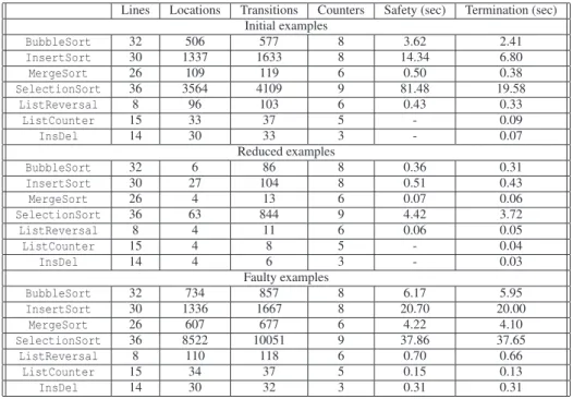
We have implemented our verification method for data-insensitive programs in a proto-type tool called L2CA (Lists To Counter Automata) [28], and performed a number of exper-iments on several textbook list sorting programs (BubbleSort, InsertSort, MergeSort, and SelectionSort), in which, for simplicity, the data comparisons were replaced by non-deterministic choices. On these examples, we have successfully checked absence of null pointer dereferences, shape invariance, as well as termination. For two of the sorting al-gorithms (BubbleSort, InsertSort), we have then also built counter automata tracking the chosen ordering predicates, which allowed us to prove sortedness of the output of these algorithms.
1.1 Related Work
The area of automated verification of programs manipulating dynamic linked data struc-tures has recently attracted quite a lot of interest. Various approaches to verification of such programs differing in their principles, degree of automation, generality, and scalability have been proposed. The approaches are based, e.g., on monadic second order logic [30], 3-valued predicate logic with transitive closure [33], separation logic [31, 21, 8, 35], other logics [14, 3, 29], automata [11, 7, 19, 12], or other symbolic representations such as [36, 4, 25, 17, 1].
Interestingly, among the works concentrating on verification of programs manipulating singly-linked lists, the idea of abstracting away the interior of list segments between in-coming edges is quite common to many works, even though they are independent and use different approaches and frameworks. Such an abstraction, of course, involves a loss of pre-cision. An idea of partially avoiding this loss by joining a counter with each abstract list segment appears, e.g., in [36] where the possible values of such counters are tracked in an abstract way using a widening operator. This suffices for verification of certain safety prop-erties, but an irrecoverable loss of precision is still involved unlike in our work. In [13], the authors use an abstract shape model with counters, but their concerns are mostly related to the decidability of a specification logic. The approaches that are the closest to ours are [5]
and its later extension [7] where an alternative translation to a bisimilar counter system is also considered, but without the extension to ordered data and without the decidability result for the case when a flat counter automaton is derived.
More recently, in [15], we have also investigated the complexity of several verification problems (e.g., for safety and termination properties) for programs with singly-linked lists. However, this line of work uses a different translation to counter automata in order to guar-antee that the obtained models are flat. This translation scheme is less general than the one considered here as it does not consider destructive update statements.
Another similar work that involves tracking the lengths of list segments and considers termination is [20]. However, this approach does not generate a counter automaton simulat-ing the original program. Instead, it first obtains invariants of the program (ussimulat-ing separation logic) and then computes the so-called variance relations that say how the invariants change within each loop when the loop is fired once more. When the computed variance relations are well-founded, termination of the program is guaranteed. Unlike our (bisimulation pre-serving) approach, the analysis of [20] fails if the initial abstraction is not precise enough. The approach of [20] was later generalised in [9] to a general framework that one can use to extend existing invariance analyses to variance analyses that can in turn be used for checking termination. Checking termination of programs with lists is tackled also by [34, 3]. In these works, ranking functions must be given manually whereas our approach is fully automated. Termination of tree manipulation programs is then considered in [22] using a translation to counter automata which is refinable via a counterexample-guided abstraction refinement (CEGAR) loop—up to the fact that the set of progress measures over the trees being ma-nipulated by the considered programs is fixed in advance. The lossy abstraction involved in this case is unavoidable as one cannot derive a bisimilar counter model like in our case for tree-manipulating programs. This is due to the fact that there are infinitely many reachable abstract shape graphs for such programs. Automated checking of termination of a program manipulating trees is also considered in [26] where the Deutsch-Schorr-Waite tree traversal algorithm was proved to terminate using a manually created progress monitor, encoded in first-order logic.
2 Programs with Lists
In this section, we define a model for imperative programs manipulating dynamic list data structures. We assume that lists are implemented using data types with one selector, i.e., next pointer (or reference) field, as it is the case in most common imperative programming languages. We consider programs without function calls and concurrency constructs, there-fore all variables are assumed to be global. We assume the lists to store elements from some ordered domain. In addition to the list data structures, the programs we consider can have (unbounded) integer variables. Simple examples of such programs include list reversion, list insertion, sorting procedures, programs counting the elements in a list, etc.
The programming model presented in this section has been simplified compared to ac-tual programming languages, such as C or C++, in the following respects: (i) the values of pointers are either allocated memory addresses or null (i.e., no dangling pointers), (ii) no pointer arithmetic is allowed, (iii) allocation statements never fail, and (iv) unreachable memory cells are automatically garbage collected.
In the first part of the paper, we assume the data stored in the lists to be completely abstracted away and we concentrate purely on pointer manipulations. In the second part, we allow a limited form of manipulation of the data contents of the lists, namely assignments of
data between memory cells and comparisons of the data contents of the cells. We concentrate mainly on checking ordering properties on programs that reorder the lists which they are given rather than change their contents. Dealing with other forms of data manipulations, such as increment or decrement, is briefly discussed at the end of the second part of the paper too—however, since dealing with such data manipulations is not the goal of this paper, we do not consider them in the supported program syntax given below.
2.1 Syntactic Definitions
The abstract syntax of the programs considered in this paper is given in Figure 2.1. We use Lab to denote a finite set of program labels (control locations), PVar to denote a fi-nite set of pointer variables, and IVar to represent a fifi-nite set of integer variables (coun-ters). The pointer variables refer to list cells. Pointers can be used in assignments such as u := null, u := w, and u := w.next; selector updates u.next := w and u.next := null; and new cell creation u := new. Assignment of data between memory cells is possible via the u.data := v.data statements. Counters can be incremented i := i + 1, decremented i := i − 1, and reset i := 0. The control structure is composed of iteration (while) statements and con-ditional (if-then-else) statements. The guards of the control statements are pointer equal-ity u= w and u = null, data comparisons u.data ≤ v.data, zero tests for counters i = 0, and boolean combinations of the above. An example of a simple program from the considered class is the list reversal program in Figure 2.
l ∈ Lab u, v, w ∈ PVar
i, j, k ∈ IVar Program:= {l : Stmnt; }∗
Stmnt:= W hileStmnt | I f Stmnt | Asgn W hileStmnt:= while Guard do {Stmnt; }∗od
I f Stmnt:= if Guard then {Stmnt; }∗!else{Stmnt; }∗"fi Asgn:= u := null | u := new | u := w | u := w.next | u.next := null
| u.next := w | u.data := v.data | i := 0 | i := i + 1 | i := i − 1
Guard:= u = v | u = null | u.data ≤ v.data | i = 0 | ¬Guard | Guard ∧ Guard | Guard ∨ Guard
Fig. 1 Abstract syntax of programs with lists
To simplify the definition of the operational semantics given below, we assume that all programs are precompiled as follows. Each pointer assignment of the form u := new, u:= w, or u := w.next is immediately preceded by an assignment of the form u := null. A pointer assignment of the form u := u.next is turned into v := u; u := null; u := v.next, possibly introducing a fresh variable v. Each pointer assignment of the form u.next := w is immediately preceded by u.next := null.
A program is said to be data-insensitive if it does not use any data assignment statements (u.data := v.data) nor data comparisons (u.data ≤ v.data).
1: j := null; 2: while i'= null do 3: k:= i.next; 4: i.next := j; 5: j:= i; 6: i:= k; 7: od
Fig. 2 A list reversal program
2.2 Concrete Operational Semantics
In order to define the concrete semantics of programs with lists, we have to formalise the notion of heaps. For our purposes, we view a heap as a graph in which nodes represent allocated memory cells, and each node has at most one successor. Moreover, we consider a partial mapping between pointer variables from PVar and graph nodes. Intuitively, if all the edges are reversed, one can imagine a heap as a set of disjoint trees in which, for each tree, there may be at most one extra edge from an arbitrary node back to the root.
In the rest of the paper, for a set A, we denote by A⊥the set A∪ {⊥}. The element ⊥ is
used to denote that a (partial) function is undefined at a given point, e.g., f(x) = ⊥. Also, for a function f : A→ B, we denote by f ↓Cthe projection of f on C, i.e., f↓C= f ∩ (C × B).
Finally, for a function f : A→ B, an element a ∈ A, and an element b ∈ B, we use the notation f[a → b] to denote a function which arises from f by setting the value of a to b, i.e., f[a → b] = ( f \ {(a, f (a))}) ∪ {(a, b)}.
Definition 1 Let.D, /0 be an infinite, totally ordered set and PVar a non-empty finite set of pointer variables. A heap is a tuple H= .N, S,V, D0 where N is a finite set of nodes, S: N→ N⊥is a successor function, V : PVar→ N⊥is a function associating to each variable
a node, and D : N→ D is a function associating to each node a data element.
The set of all heaps using variables from PVar is denoted byH(PVar). We denote the fact that S(n1) = n2 in H by n1−→
H n2. We use u−→H nto denote the formula∃m . V (u) =
m ∧ m −→
H n. Here, H might be omitted when it is clear from the context. We denote by ∗
−→
H
the reflexive and transitive closure of−→
H. A node n is said to be a cut-point in H, denoted as
cutH(n), if it has two predecessors or it is pointed to by a variable. Formally, let
cutH(n) : ∃n1, n2∈ N . n1'= n2∧ S(n1) = S(n2) = n ∨ ∃u ∈ PVar . V (u) = n.
When a node n is removed from a heap, or when its successor link is changed, some successors of n may become unreachable from the pointer variables. Due to the implicit garbage collection, such nodes are removed from the heap. The set of nodes whose lifetime depends exclusively on their reachability through the node n is denoted as depH(n) in the
following. Formally, for a heap H= .N, S,V, D0 and n ∈ N: depH(n) =
#
m∈ N | ∀u ∈ PVar. ¬$u−−−−−−−−→∗
.N,S[n→⊥],V,D0 m
%&
The state of a program with lists is a triple.l, H, ι0 where l ∈ Lab is the current program label, H∈H(PVar) is the current heap configuration, and ι : IVar → Z is the current valuation of counter variables. A pointer assignment statement s between locations l and
l3 (denoted l : s; l3) changes the state from.l, H, ι0 to .l3, H3, ι0, where H3is a new heap
configuration such that H−→ Hs 3in conformance with the rules presented in Figure 3.
Rules C1, C2, and C3describe the effect of assigning null to a pointer variable u. If u
is not allocated, then there is no change in the heap (C1). Otherwise, the location n pointed
to by u and its dependent nodes are removed if and only if it is not reachable from another variable than u (C2, C3). The assignment between two pointer variables u and w assumes that
uis previously null (C4). Analogously, the allocation statement described by (C5) assumes
that the allocated variable was previously null. Notice that the data element of the newly allocated cell is chosen randomly from the data domain D. Further, setting the next field of an allocated memory cell to null may generate garbage cells, which must be collected (C9).
Notice that assigning the next field to another pointer variable is possible only provided that it was previously set to null (C10). When a null pointer dereference is encountered, the heap
is changed to a special sink heap configuration Herr(C6, C8, C11), Herr'∈H(PVar).
A pointer equality test u= v evaluates to true in a heap H = .N, S,V, D0 iff V (u) = V (v). Also, u= null is true iff V (u) = ⊥. A data comparison u.data ≤ v.data leads to Herr iff
V(u) = ⊥ or V (v) = ⊥. Otherwise, it evaluates to true iff D(V (u)) ≤ D(V (v)). The seman-tics of tests and updates on counters is as usual, and so is the semanseman-tics of the conditional statements and loops.
V(u) = ⊥ H−−−−−−→ Hu:= null
C1
V(u) '= ⊥ ∃w ∈ PVar \ {u} . w−→∗
H V(u)
H−−−−−−→ .N, S,V [u → ⊥], D0u:= null C2
V(u) = n ∈ N ∀w ∈ PVar \ {u} . ¬'w−→∗
H n ( N3= N \ ({n} ∪ depH(n)) H−−−−−−→ .Nu:= null 3, S ↓N3,V [u → ⊥], D ↓N30 C3 V(u) = ⊥ H−−−−−→ .N, S,V [u → V (w)], D0u:= w C4
V(u) = ⊥ n'∈ N is a fresh node d∈ D H−−−−−−→ .N ∪ {n}, S[n → ⊥],V [u → n], D[n → d]0u:= new C5 V(w) = ⊥ H−−−−−−−−→ Hu:= w.next err C6 V(u) = ⊥ V (w) = n ∈ N H−−−−−−−−→ .N, S,V [u → S(n)], D0u:= w.next C7 V(u) = ⊥ H−−−−−−−−−−→ Hu.next := null err
C8 V(u) = n ∈ N N3= N \ depH(n) H−−−−−−−−−−→ .Nu.next := null 3, S[n → ⊥] ↓ N3,V, D ↓N30 C9 V(u) = n ∈ N S(n) = ⊥ H−−−−−−−−→ .N, S[n → V (w)],V, D0u.next := w C10 V(u) = ⊥ or V (v) = ⊥ H−−−−−−−−−−−−→ Hu.data := v.data err
C11 V(u) = n ∈ N V (v) = m ∈ N H−−−−−−−−−−−−→ .N, S,V, D[n → D(m)]0u.data := v.data C12 Herr−→ Hs err C13
3 Counter Automata
A counter automaton with n counters is a tuple A= .Q, X, q0, →0 where Q is a finite set
of control states, q0∈ Q is an initial state, X = {x1, . . . , xn} are counter variables, and →∈
Q× Φ × Q are transitions where Φ is the set of Presburger formulae with free variables from{xi, x3i| 1 ≤ i ≤ n}. A configuration of a counter automaton with n counters is a tuple
.q, ν0 where ν is a mapping from X to N. The set of all configurations is denoted byC. Let FV(ϕ) denote the set of free variables of a formula ϕ. The transition relation−→⊆C C×C
is defined by letting(q, ν)−→ (qC 3, ν3) iff there exists a transition q−→ qϕ 3 such that ifσ is
an assignment of FV(ϕ) where σ(x) = ν(x) and σ(x3) = ν3(x), we have that ϕ(FV (ϕ)σ)
holds andν(x) = ν3(x) for all variables x with x3'∈ FV (ϕ). A run of A is a sequence of
configurations(q0, ν0), (q1, ν1), (q2, ν2) . . . such that (qi, νi)
C −
→ (qi+1, νi+1) for each i ≥ 0.
Definition 2 Let A= .Q, X, q0, →0 be a counter automaton where X = {x1, . . . , xn} are
counter variables that range over positive integers. A is said to be linear if all its transitions are of the formϕ(X) ∧!1≤i≤nx3i= fi(X) where ϕ is a formula of Presburger arithmetic and
fi= ∑nj=1ai jxj+ bi, 1≤ i ≤ n, are linear functions with integer coefficients. Moreover, A is
said to be positive if ai j≥ 0 for all 1 ≤ i, j ≤ n. A is also said to be restrictive if there exists a
constantα ∈ N such that for each control state q ∈ Q, on each run π that visits q, the sum of values taken by the counters, ∑n
i=1xi, increases by at mostα between any two consecutive
times when the control state is q.
The control graph of a counter automaton A is the graph having as vertices the set Q of control states, and, for any two states q and q3, there is an edge between q and q3in the control graph if and only if there exists a transition q−→ qϕ 3in A. A counter automaton is said to be
flatif its control graph has no nested loops. A control path scheme is a regular expression over the edges of a control graph describing a set of paths between two control states. For a flat counter automaton A= .Q, X, q0, →0 and any two control states q, q3∈ Q, the set of
paths between q and q3is a finite union of path schemes of the form L∗1S1L∗2S2. . . Sn−1L∗n
where Liare possibly empty elementary loops (i.e., paths starting and ending in the same
control state, with no repeated states in between), and Siare sequential paths between loops.
We use q−→ qE 3to denote that E is a control path scheme describing a set of paths between
the states q and q3.
Theorem 1 The problems of reachability and termination for flat linear positive restrictive counter automata are decidable.
Proof Let A= .Q, X, q0, →0 be a flat counter automaton where X = {x1, . . . , xn}. We reduce
the problems of reachability and termination for flat counter automata to the problem of computing the relation between input and output values of the counters, for any execution path. This amounts essentially to computing the transitive closure of a transition relation labelling a loop q−→ . . . −→ q in the automaton, where the input values of the counters are restricted by an initial condition Iq(X). This initial condition summarises all possible
execu-tions up to the beginning of the loop. Formally, we have the following for each control state q∈ Q: Iq(X) = ∃X0∃X03. . . ∃Xn−1. " q0 L∗ 1S1L∗2S2...Sn−1L∗n −−−−−−−−−→q λ∗1(X0, X03) ∧ σ1(X03, X1) ∧ . . . ∧ σn−1(Xn−23 , Xn−1) ∧ λ∗n(Xn−1, X)
whereλi is the transition relation of Li, 1≤ i ≤ n, and σi is the transition relation of Si,
1≤ i < n, respectively. Here, R∗denotes the transitive closure of a relation R.
Hence we can restrict our attention w.l.o.g. to one self-loop of the form q−→ q, param-φ eterised by an initial condition on counters Iq(X). The transition relation φ is of the form
ϕ(X) ∧ X3= f (X) where f (X) = X · A + B is an affine transformation, according to
Defini-tion 2. Here, A∈ Z|X|×|X|is a square matrix and B∈ Z|X|is a row vector. We assume w.l.o.g.
that all columns of A are linearly independent, for else the value of some counters are linear combinations of the other counters and could be encoded as a part ofϕ. As a consequence, Ais invertible, i.e., there exists A−1∈ Q|X|×|X|such that AA−1= A−1A= 1, where 1 is the
identity matrix.
Let x(m)i denote the value of the counter xiat the m-th visit of control state q. We have
the following for all m≥ 0:
n
∑
i=1 x(m+1)i − n∑
i=1 x(m)i ≤ α n∑
i=1 ( fi(x(m)1 , . . . , x(m)n ) − x (m) i ) ≤ α n∑
i=1 ( n∑
j=1 ai jx(m)j + bi− x(m)i ) ≤ α n∑
i=1 ( n∑
j=1 aji− 1)x(m)i ≤ α − n∑
i=1 biSince all coefficients are positive, we have ∑n
j=1aji≥ 0 for all 1 ≤ i ≤ n. If it is the case
that ∑nj=1aji= 0 for some 1 ≤ i ≤ n, i.e., all coefficients of xiare zero, then xiis not used
in computing the next values of X , and we can eliminate xifrom the transition relation as
described in the following.
Let X = X \ {xi}, and f (X) be the projection of f onto X. Then the loop executes as
follows:
Iq(X(0)) ∧ ϕ(X(0)) ∧ X(1)= f (X(0))
ϕ(X(1)) ∧ X(2)= f (X(1)) ϕ(X(2)) ∧ X(3)= f (X(2))
. . . which is equivalent to:
∃xi(0). [Iq(X(0)) ∧ ϕ(X(0))] ∧ X(1)= f (X(0))
∃x(1)i ∃Xp. [X(1)= f (Xp) ∧ ϕ( f (Xp))] ∧ X(2)= f (X(1))
∃x(2)i ∃Xp. [X(2)= f (Xp) ∧ ϕ( f (Xp))] ∧ X(3)= f (X(2))
. . . The equivalence betweenϕ(X(i))∧X(i+1)= f (X(i)) and ∃x(i)
i ∃Xp. [X(i)= f (Xp)∧ϕ( f (Xp))]∧
X(i+1)= f (X(i)), for i > 0, can be seen by the fact that X(i)= X(i−1)A+ B (by the previous
that Xp and X(i−1) are the same values. But since A is invertible, we have Xp= X(i−1)=
(X(i)− B)A−1.
Hence it is enough to unfold the loop once and consider the first transition separately. Obviously, all incoming and outgoing transitions will have to be duplicated, but this does not change the flatness of the control structure. The result is a machine with the following control structure and with counters X :
q0 ∃xi. [Iq(X)∧ϕ(X)] ∧ X3= f (X) −−−−−−−−−−−−−−−−→ q1 q1 ∃xi∃Xp. [X= f (Xp)∧ϕ( f (Xp))] ∧ X3= f (X) −−−−−−−−−−−−−−−−−−−−−−→ q1
Obviously, all properties (reachability, termination) of the original machine are preserved by the transformation.
We can therefore restrict w.l.o.g. to the case where ∑n
j=1aji> 0 for all 1 ≤ i ≤ n. Then
either: – ∑n j=1aji> 1, in which case 0 ≤ x(m)i ≤ α−∑n i=1bi ∑n j=1aji−1, or – ∑n
j=1aji= 1, i.e., aki= 1 for some k and aji= 0 for all j '= k.
This (static) case split partitions the set of counters X into two disjoint subsets: a set of counters Y for which the first case applies and which are bounded by a constant throughout the execution of the automaton, and a set of counters Z for which the second case applies and which must occur exactly once in the computation of X3; i.e., for each z∈ Z there exists exactly one x∈ X such that x3= z + g where g is a linear combination not involving z.
We now distinguish three cases. (1) If x∈ Y , the value of z is also bounded by a constant. Otherwise, (2) if x∈ Z and g contains another occurrence of a variable t from Z, this means that there exists another variable s from Z whose next value depends only on values from Y, or else there would be a variable from Z occurring in two places. In this case, the value of s is also bounded by a constant. The last case (3) is z3= t + g(Y ) for z,t ∈ Z. In the first two cases, the partition can be modified by moving bounded variables from Z to Y until a fixpoint is reached.
According to the resulting partition (Y, Z), the values taken by the counters at each iteration have the following properties:
– Y range over an effectively computable finite set of values V= {v1, . . . , vN},
– Y3are linear combinations of Y ,
– Z3= Z + δ where δ are linear combinations of Y .
Since the values taken by Y are bounded, they can be encoded in the control of a new counter machine. Given a self loop q−−−→ q where ψ =ϕ ∧ ψ !1≤i≤nx3i= fi(X) is the same as in
Definition 2, and a partition of the counters into(Y, Z) that satisfies the requirements above, we can build a counter machine Asim= .V||Y ||∪ {q0}, Z, q0, δsim0 where δsim is defined as
follows: – q0
6
−→ v if v ∈ V||Y ||is an initial tuple of values for Y ,
– for all v, v3∈ Z||Y ||and w, w3∈ Z||Z||, we have:
v ϕ[v/Y ] ∧ ψ[v/Y,v
3/Y3,Z+δ/Z3] ∧ Z3=Z+δ
−−−−−−−−−−−−−−−−−−−−−−→
Asim
Notice that the new transition relationδsimis deterministic since v3andδ are linear
com-binations of v. This means that the control structure of Asimis in fact a loop, corresponding
to a finite number of unfoldings of q−−−→ q. The new machine simulates the original loopϕ ∧ ψ in the sense that any execution of the former corresponds to an execution of the latter and vice-versa. Moreover, the set of configurations of the original loop is in a one-to-one relation with the set of configurations of Asim.
Let M be the length of the loop constituting the control of Asim. This is an effectively
computable constant, bounded by N|y|, the number of control states. In other words, Asim
is of the form: v0 ϕ0∧Z3=Z+δ0 −−−−−−−→ v1 ϕ1∧Z3=Z+δ1 −−−−−−−→ v2. . . −→ vM−1 ϕM−1∧Z3=Z+δM−1 −−−−−−−−−−→ v0whereϕi=
ϕ[vi/Y ] ∧ ψ[vi/Y, v3i/Y3, Z + δi/Z3]. The relation between the input Z and output Z3values of
the counters of Asimcan now be defined by the Presburger formula
∃l ≥ 0 .#M−1j=0 Z3= Z + l ∑M−1i=0 δi+ ∑i=0j δi∧ (1)
∀0 ≤ m < lM + j . ϕm mod M(Z +Mm∑M−1i=0 δi+ ∑mi=0mod Mδi) (2)
where Mm denotes integer division. Intuitively, the formula from the first row gives the dif-ference between Z3and Z whereas the second one ensures that the guards are satisfied all along the way. Notice thatϕj(Z +Mm∑M−1i=0 δi+ ∑mi=0mod Mδi), 0 ≤ i < M, are indeed formulae
of Presburger arithmetic provided thatϕ is.
Given a flat linear positive restrictive automaton, one can compute the above formula for each individual loop. The reachability and termination problems for these automata can
be reduced to satisfiability of Presburger formulae. 78
4 Abstract Semantics of Programs with Lists
A common way of representing heaps compactly consists in mapping an entire list segment with no edges incoming into the middle of it into a special (abstract) node. This idea con-stitutes the basis of our abstraction too. LetN be a set of abstract nodes and X be a set of counter variables, one for each node. We shall first define the abstract structure of heaps. Definition 3 An abstract structure is a tuple H= .N, S,V 0 where:
– N⊆N is a set of abstract nodes, – S : N→ N⊥is a successor mapping, and
– V : PVar→ N⊥is a variable mapping.
A cut-point in H is a node n∈ N such that there exist n1, n2∈ N with n1'= n2and S(n1) =
S(n2) = n or there exists u ∈ PVar with V (u) = n. An abstract structure is said to be in
normal formiff each node n∈ N is a cut-point in H that is reachable from some u ∈ PVar, i.e., u−→∗
H
n.
Intuitively, each abstract node corresponds to a set of concrete nodes, and the counter corresponding to each node gives the number of nodes in this set. For abstract structures in normal form, we do not allow sequences of successive abstract nodes that are neither pointed by a variable, nor have their in-degree greater than one. This condition is needed in order to ensure that any such abstract structure defined over a finite set of variables is finite. We useH(PVar) to denote the set of all abstract structures with variables from PVar and
Hn f(PVar) to denote the subset ofH(PVar) containing abstract structures in normal form
Lemma 1 Let PVar= {u1, . . . , un} be a set of variables, and H = .N, S,V 0 be an abstract
structure in normal form such that dom(V ) ⊆ PVar. Then ||N|| ≤ 2n. Moreover, ||Hn f(PVar)||
is of the order of2Θ(nlog(n)).
Proof We show that||N|| ≤ 2n by induction on the cardinality n of PVar. For n = 1, it is obvious that the abstract structures in normal form can have at most two nodes: either there is no node at all, or the unique variable points to a node which points to null or to itself, or the variable points to a first node which points to a second node which points to itself. Now, let us suppose that||N|| ≤ 2n holds for abstract structures in normal form with n variables. If we have one more variable un+1, it either points to a part of the heap completely separated
from the other n variables, or not. In the former case, there can be at most two more nodes using the same reasoning as in the base case. In the latter case, there can be at most one node m (pointed to by un+1) which is not reachable from the other variables. Furthermore,
the successor of m must be a cut-point m3. If m3is pointed to by a variable, we can remove m and un+1and apply the induction hypothesis on the remaining heap which is in normal form
since m3is still a cut-point. The same can also be done if m3is pointed to by at least two other nodes distinct from m. If m3is pointed to by exactly one other node m33, it is no more a cut-point after removing un+1and m. However, if we remove m3by letting m33point to the
successor of m3, then the obtained heap is in normal form and we can apply the induction hypothesis on it yielding the desired bound.
For the second part, we compute an upper and lower bound on the number of heaps with 2n nodes. For the upper bound, we note that an abstract structure, not necessarily in normal form, with 2n nodes can be uniquely encoded by the following mappings:
– s :{1, . . . , 2n} → {1, . . . , 2n, ⊥} is the partial successor function, i.e., s(n) = ⊥ iff the node n has no successor,
– v :{1, . . . , n} →{ 1, . . . , 2n, ⊥} maps variables into nodes, i.e., v(i) = ⊥ iff the i-th vari-able is undefined.
Taking this into account, the number of abstract structures, not necessarily in normal form, with 2n nodes is at most(2n + 1)2n· (2n + 1)n= (2n + 1)3n. At the same time, this formula
gives an upper bound on the number of abstract structures in normal form with 2n nodes or less as well. This is because for each abstract structure H in normal form with m< 2n nodes there is at least one abstract structure not in normal form which has 2n nodes and which is equal with H, up to having 2n− m garbage nodes (i.e., nodes unreachable from the pointer variables).
For the lower bound, we consider only trees with n nodes, all of which are pointed to by a variable. The number of unlabelled trees with n nodes is the Catalan number Cn=n!(n−1)!(2n−2)!,
and the number of possible variable assignments is n!. Hence the number of labelled trees is n· (n + 1) · . . . · (2n − 2) ≥ nn−1. So nn−1 is a lower bound on the number of abstract
structures in normal form with 2n nodes. Hence the number of abstract structures in normal form pointed to by n pointer variables is of the order of 2Θ(nlog(n)). 78 Let us now define our first abstraction function, denoted by αs, that maps concrete
heaps into abstract structures. Given a concrete heap H = .N, S,V, D0, let RH ⊆ N × N
be a relation on the set of nodes defined such that n1RHn2 holds for any n1, n2∈ N iff
n1−→
H n2∧ ¬cutH(n2). We denote by ∼H the reflexive, symmetric, and transitive closure
of RH. The H subscript shall be further omitted for simplicity. For a node n∈ N, we denote
by[n] the equivalence class of n with respect to ∼, also referred to as a list segment. The quotient heap H/∼= .N/∼, S/∼,V/∼0 is defined as follows:
– N/∼= {[n] | n ∈ N},
– for all n, m ∈ N, S/∼([n]) = [m] iff ∃n0∈ [n] ∃m0∈ [m] . S(n0) = m0∧ cutH(m0),
– for all u∈ PVar, n ∈ N, V/∼(u) = [n] iff V (u) ∈ [n], and
– S/∼and V/∼are undefined, otherwise.
Note that S/∼and V/∼are well defined partial functions. Indeed, assume that for some n∈ N,
S/∼maps[n] into two different equivalence classes, call them [m] and [p]. This would imply
that there are two nodes n1, n2∈ [n] such that n1−→
H m0and n2−→H p0where m0∈ [m] is the
cut-point at the beginning of the list segment[m], and p0∈ [p] is the cut-point at the beginning
of the list segment[p]. Since [m] and [p] are different segments, m0'= p0. Now, note that
since nodes in a list segment are linked together, each of them has just one successor, and only the first node of a list segment is a cut-point, only the last node of a list segment may point to a cut-point. However, then it must be the case that n1= n2, and hence also m0= p0,
which is a contradiction. The argument for V/∼is straightforward.
In Figure 4 (a), an example of a concrete heap with its cut-points is given. For example, the nodes n1and n2form an equivalence class.
2 1 2 1 3 3 (b) (a) u v x y y x n3 6 u n34 n31 n35 n33 n32 n1 n2 n3 n7 n8 n9 n10 n11 n12 n4 n5 n6 v
Fig. 4 Concrete and abstract structures. The cut-points are n1, n3, n4, n7, n9and n10.
For an equivalence class[n] ∈ N/∼, we denote by hd([n]), tl([n]) the head and tail of the
list segment, respectively, and by[n] ◦ [m] the concatenation of two list segments.
Definition 4 Let H= .N, S,V, D0 be a concrete heap and H/∼= .N/∼, S/∼,V/∼0 its quotient.
An abstract structure H= .N, S,V 0 is said to be a structural abstraction of H if and only if there exists a bijective functionβ : N/∼∪ {⊥} → N ∪ {⊥} such that β(⊥) = ⊥, and for all
u∈ PVar:
– S(β([n])) = β(S/∼([n])) and
– V(u) = β(V/∼(u)).
Note that an abstract structure that is a structural abstraction of some concrete heap is necessarily in normal form. Two abstract structures that differ only in the naming of nodes and counter variables are semantically equivalent in the sense that they are abstractions of the same set of concrete heaps. In practice, this increases the number of abstract structures generated by a symbolic state exploration tool. This problem can be overcome by choosing a canonical representation of abstract structures as described, e.g., in [23].
We define the structural abstraction functionαs : H(PVar) →Hn f(PVar), αs(H) = H
iff H is the canonical representative of a structural abstraction of H. Dually, the concretisa-tionof an abstract structure H is the set of concrete heaps whose structural abstraction is H, i.e.,γs(H) = {H | αs(H) = H}.
Furthermore, let H= .N, S,V 0 be an abstract structure in normal form and ν : N → N+a
mapping of nodes to positive natural numbers. Byν(H), we denote the set of concrete heaps obtained by replacing each node n∈ N by a list segment of length ν(n) and data arbitrarily chosen from D. Clearly,γs(H) =
$
For example, the concrete heap in Figure 4 (a) is one possible concretisation of the abstract structure in Figure 4 (b), for the valuation:ν(n3
1) = 2, ν(n32) = 1, ν(n33) = 3, ν(n34) =
2,ν(n3
5) = 1, ν(n36) = 3.
4.1 Data-Insensitive Programs
This section is devoted to a description of counter automata that abstract the behaviour of data-insensitive programs with lists. We formalise correctness of our construction by prov-ing bisimulation between the semantics of a data-insensitive list program and the semantics of a counter automaton. This entails a strong preservation of temporal logic properties. In particular, safety and termination are strongly preserved by the counter automata, meaning that one can prove as well as disprove safety and termination properties of the programs based on the behaviour of their representation by the counter automata.
Consider a data-insensitive list program with k pointer variables and l counter variables, i.e.,||PVar|| = k and ||IVar|| = l. We construct a counter automaton A = .Q, X,−→0 withs 2k+ l counters as follows. The control states Q of the counter automaton are elements of the set Lab× (Hn f(PVar) ∪ {Herr}) where Herr'∈H(PVar) is a special sink error state. Let N =${N | .N, S,V 0 ∈Hn f(PVar)} be the set of nodes used in the structural abstraction. The counters are X = {xn | n ∈N} ∪ IVar, i.e., one counter for each node used in the
structural abstraction plus the counter variables from the original program. The transitions are given by triples q−→ qϕ 3such that (1) q= .l, H0, (2) q3= .l3, H30, (3) there is a statement
l: s; l3in the program, and (4) it is the case that H−→ϕ
s H
3where the relation−→ϕ
s is described
by the structural rules given in Figures 5 and 7. More precisely, Figures 5 and 7 contain rules Aiwhich correspond to the rules Cifrom Figure 3. Sometimes several rules in the abstract
semantics are needed for one rule in the concrete semantics. The rules for data manipulation (C11, C12) are not needed in the abstract semantics for data-insensitive programs. In order to
simplify the treatment of the different cases in the rules of Figures 5 and 7, they are based on two low-level operations for merging and splitting abstract nodes, which are explained in the following paragraphs.
Intuitively, when the effect of some pointer manipulating statement is simulated over an abstract structure in normal form, it may happen that we obtain an abstract structure H= .N, S,V 0 in which there are two abstract nodes n and m such that m is a successor of n, and m is not a cut-point. In such a case, we need to merge the two abstract nodes n and m in order to re-normalise the abstract structure. For this purpose, we use the merging function µ :H(PVar)×N×N →H(PVar) defined as µ(H, n, m) = .N3, S↓
N3[n → S(m)],V 0 where
N3= N \ {m}.
Furthermore, when simulating the effect of the statement u := w.next, we need to split the abstract node n pointed to by w into two nodes n and m provided that the value of its corresponding counter is greater than one (i.e., xn> 1). For this purpose, we use the splitting
function σ : H(PVar) ×N ×N →H(PVar) defined as σ(H, n, m) = .N ∪ {m}, S3,V 0
where S3='S\ {(n, S(n))}(∪ {(n, m), (m, S(n))}.
The semantics of tests (u= v and u = null) is similar to the concrete case, and the same holds for the conditional statements, while loops, and counter manipulating statements.
For an illustration of the translation, the reader is referred to the list reversal example in Figure 8.
Now we can state the main theorem of this section, establishing bisimilarity between a data-insensitive program manipulating lists and the counter automaton modelling it. Given
V(u) = ⊥ H−−−−→true
u:=null H
A1
∃w ∈ PVar \ {u} V(w) = V (u) '= ⊥ H−−−−→true
u:=null .N, S,V [u → ⊥]0
A2
V(u) = n ∈ N ∀w ∈ PVar \ {u} . V (w) '= n ∃m, p ∈ N . p '= m ∧ S(m) = S(p) = n
H−−−−→true
u:=null .N, S,V [u → ⊥]0
A32
V(u) = n ∈ N ∀w ∈ PVar \ {u} . V (w) '= n ∃m ∈ N \ {n} . S(m) = n ∀p ∈ N \ {m} . S(p) '= n H x 3 m=xm+xn −−−−−−→ u:=null µ(.N, S,V [u → ⊥]0, m, n) A332
V(u) = n ∈ N ∀w ∈ PVar \ {u} . w '−→∗
H n S(n) ∈ {⊥, n} N3= N \ {n} H−−−−→true u:=null .N 3, S ↓ N3,V [u → ⊥]0 A3
V(u) = n ∈ N ∀w ∈ PVar \ {u} . w '−→∗
H n S(n) = m ∈ N \ {n} ∃w ∈ PVar \ {u} . V (w) = m N3= N \ {n} H−−−−→true u:=null .N 3, S ↓ N3,V [u → ⊥]0 A33
V(u) = n ∈ N ∀w ∈ PVar \ {u} . w '−→∗
H n S(n) = m ∈ N \ {n} ∀w ∈ PVar \ {u} . V (w) '= m ∃p, q ∈ N \ {n} . p '= q ∧ S(p) = m ∧ S(q) = m N3= N \ {n} H−−−−→true u:=null .N 3, S ↓ N3,V [u → ⊥]0 A333
V(u) = n ∈ N ∀w ∈ PVar \ {u} . w '−→∗
H n S(n) = m ∈ N \ {n} ∀w ∈ PVar \ {u} . V (w) '= m ∃p ∈ N \ {n, m} . S(p) = m ∀q ∈ N \ {n, p} . S(q) '= m N3= N \ {n} H x 3 p=xp+xm −−−−−−→ u:=null µ(.N 3, S ↓ N3,V [u → ⊥]0, p, m) A3333
V(u) = n ∈ N ∀w ∈ PVar \ {u} . w '−→∗
H n S(n) = m ∈ N \ {n} ∀w ∈ PVar \ {u} . V (w) '= m ∀p ∈ N \ {n, m} . S(p) '= m N3 = N \ {n, m} H−−−−→true u:=null .N 3, S ↓ N3,V [u → ⊥]0 A33333
Fig. 5 The data-insensitive counter automata semantics of u := null on an abstract structure H = .N, S,V 0 in normal form—see Fig. 6 for an illustration of the different cases
a data-insensitive, list manipulating program P, let.S,−→0 be its concrete semantics withc the set of statesS= Lab ×H(PVar) × (IVar → Z) and−→ being its transition relation. Letc
S= Q×(X → Z) be the set of all configurations of the corresponding counter automaton and
s
−
→ its transition relation. Let!s⊆S×Sbe the relation defined such that(l, H, ι)!s(l, H, ν) holds for a concrete heap H= .N, S,V, D0, an abstract structure H = .N, S,V 0 in normal form, program labels l and l, and valuationsι : IVar → Z and ν : X → Z iff one of the two following cases happens:
– l= l, H is a structural abstraction of H based on a bijection β : N/∼∪ {⊥} → N ∪ {⊥}
in accordance with Definition 4,ν ↓IVar= ι, and ∀n ∈ N . ν(xn) = ||β−1(n)||; or
– l= l ∧ H = Herr ∧ H = Herr.
Theorem 2 The relation!sis a bisimulation between.S,−→0 and .c S,−→0.s
Proof We prove the theorem by considering all possible different statements in the program. The case of Herr and Herris trivial. Suppose that we are given(l, H, ι)!s(l, H, ν) such that
u,w (a) A2 u m n p u m n or (b) A32 u m n (c) A332 u n u n or (d) A3 u n m w (e) A33 u n m p q u n m p or (f) A333 u n p m (g) A3333 u n m (h) A33333
Fig. 6 An illustration of the different cases of the counter automata semantics of u := null from Fig. 5
H'= Herr, and letβ : N/∼∪ {⊥} → N ∪ {⊥} be the bijection from Definition 4 linking H/∼
and H.
We need to show that for each statement s, (1)(l, H, ι)−→ (ls 3, H3, ι3) implies (l, H, ν) s
− → (l3, H3, ν3) and (l3, H3, ι3)! s(l3, H 3 , ν3), and (2) (l, H, ν)−→ (ls 3, H3, ν3) implies (l, H, ι) s − → (l3, H3, ι3) and (l3, H3, ι3)! s(l3, H 3 , ν3).
For statements which are assignments involving integer variables, this is obvious. For statements which are guards involving integer variables, this is also obvious. For guards of the type u= v involving pointer variables, this follows directly from Claim (1) proven below. The case of guards of the type u= null is analogical.
Claim (1)Given an abstract structure H= .N, S,V 0 such that H is a structural abstraction of a concrete heap H= .N, S,V, D0, we have for all u, w ∈ PVar, V (u) = V (w) iff V (u) = V (w). Proof V(u) = V (w) = ⊥ iff V/∼(u) = V/∼(w) = ⊥ iff V (u) = V (w) = ⊥, by Definition 4.
If V(u) = V (w) '= ⊥, then V (u) = V (w) '= ⊥ follows. Dually, if V (u) = V (w) = n, then V/∼(u) = V/∼(w) = β−1(n). Then either V (u) = V (w), or V (u) '= V (w) and V (u) ∼HV(w).
The latter case leads to a contradiction due the fact that V(w) is a cut-point. 78
For the other cases, we need another property.
Claim (2)Given a concrete heap H= .N, S,V, D0 and its structural abstraction H based on a bijectionβ, for all n, m ∈ N such that cutH(m) and cutH(n), n
∗ −→ H miffβ([n]) ∗ −→ H β([m]).
Proof “⇒” We show that for all n, m ∈ N such that cutH(m) and cutH(n), n−→∗
H mimplies
β([n])−→∗
H
β([m]) by induction on the number c of cut-points different from n and m which appear along the shortest path from n to m. For c= 0, we have two cases: First, n = m, in which case, we trivially haveβ([n]) = β([m]). Second, n '= m. In this case, there must be some n3∈ [n] such that n−→∗
H n 3−→
H m, and we are done since[n] = [n 3] and S
/∼([n3]) = [m].
Assume now that the implication holds for all pairs of cut-points linked by shortest paths of length at most c. Let n and m be cut-points linked by a shortest path of length c+ 1. Then,
V(u) = ⊥ H−−−→true u:=w .N, S,V [u → V (w)]0 A4 V(u) = ⊥ n∈N\ N H x 3 n=1 −−−−→ u:=new .N ∪ {n}, S[n → ⊥],V [u → n]0 A5 V(w) = ⊥ H−−−−−→true u:=w.next Herr A6 V(u) = ⊥ V(w) = n ∈ N H−−−−−→xn=1 u:=w.next .N, S,V [u → S(n)]0 A7 V(u) = ⊥ V(w) = n ∈ N m∈N\ N3 H xn>1 ∧ x 3 m=xn−1 −−−−−−−−−−→ u:=w.next σ(.N, S,V [u → m]0, n, m) A37 V(u) = ⊥ H−−−−−−−→true u.next:=null Herr A8 V(u) = n ∈ N S(n) ∈ {⊥, n} H x 3 n=1 −−−−−−−→ u.next:=null .N, S[n → ⊥],V 0 A9 V(u) = n ∈ N S(n) = m ∈ N \ {n} ∃v ∈ PVar \ {u} . V (v) = m H x 3 n=1 −−−−−−−→ u.next:=null .N, S[n → ⊥],V 0 A39 V(u) = n ∈ N S(n) = m ∈ N \ {n} ∀v ∈ PVar . V (v) '= m ∃p, q ∈ N \ {n} . p '= q ∧ S(p) = S(q) = m H x 3 n=1 −−−−−−−→ u.next:=null .N, S[n → ⊥],V 0 A339 V(u) = n ∈ N S(n) = m ∈ N \ {n} ∀v ∈ PVar . V (v) '= m ∃p ∈ N \ {n, m} . S(p) = m ∀q ∈ N \ {n, p} . S(q) '= m H x 3 n=1 ∧ x3p=xp+xm −−−−−−−−−−−→ u.next:=null µ(.N, S[n → ⊥],V 0, p, m) A3339 V(u) = n ∈ N S(n) = m ∈ N \ {n} ∀v ∈ PVar . V (v) '= m ∀p ∈ N \ {n, m} . S(p) '= m N3 = N \ {m} H x 3 n=1 −−−−−−−→ u.next:=null .N 3, S ↓ N3[n → ⊥],V 0 A33339 V(u) = n ∈ N S(n) = ⊥ H−−−−−→true u.next:=w .N, S[n → V (w)],V 0 A10 Herr true −−→ s Herr A13
Fig. 7 The data-insensitive counter automata semantics of program statements other than u := null
there must be some cut-point n3∈ N such that n−→∗
H n 3−→
H mand there is no further cut-point
on the shortest path between n3and m. We are done by considering the induction hypothesis
over n−→∗
H n
3and the base case over n3−→ H m.
“⇐” We show that for all n, m ∈ N such that cutH(m) and cutH(n), β([n]) ∗
−→
H
β([m]) implies n−→∗
H mby induction on the length c of the shortest path betweenβ([n]) and β([m])
in H. If c= 0, it must be the case that n = m since both n and m are cut-points, and we are done. If c= 1, there must be some n3∈ [n] such that n3−→
H m. Since n ∗ −→ H n 3, we have n ∗ −→ H m.
Assume now that the implication holds for all paths of length up to c. Since any path of length c+ 1 can easily be split to two paths of length at most c, we may apply the induction
hypothesis and we are done. 78
We now consider all statements involving pointer variables. We suppose that they go from l to l3.
– V(u) = ⊥. We have V (u) = ⊥ iff V (u) = ⊥, by Definition 4. Therefore, rule C1applies to
H(without changing it) iff the analogical rule A1applies to H (again, without changing
it), and it is clear that(l3, H, ι)!
s(l3, H, ν).
– V(u) '= ⊥ and ∃w ∈ PVar \ {u} . V (w) = V (u). We have V (u) = V (w) '= ⊥ iff V (u) = V(w) '= ⊥, by Claim (1). In this case, rule C2applies to H iff rule A2applies to H, and
it can easily be checked that(l3, .N, S,V [u → ⊥], D0, ι)!
s(l, .N, S,V [u → ⊥]0, ν).
– V(u) '= ⊥ and ∀w ∈ PVar \ {u} . V (w) '= V (u) and ∃w ∈ PVar \ {u} . w−→∗
H V(u). Let
w∈ PVar \ {u} be any variable such that w−→∗
H V(u). Since V (u) and V (w) are
cut-points, we have V(w)−→∗
H V(u) iff V (w) ∗
−→
H V(u), by Claim (2). Moreover, V (u) '= V (w),
by Claim (1), and rule C2applies to H iff rule A32or rule A332 applies to H. We have to
distinguish two cases—either the node V(u) is still a cut-point after u := null or not: – In the former case, rule C2applies to H iff rule A32applies to H. Since there is no
change in H nor H (except for the value of u that is set to⊥ in both cases) and there is no change inι and ν, we are done.
– In the latter case, rule C2applies to H iff rule A332applies to H. Let H3= .N, S,V [u →
⊥], D0 be the heap obtained after rule C2and H3= .N3, S3,V30 be the abstract
struc-ture obtained after rule A332. Let V(u) = n and let m ∈ N be such that w ∗
−→
H m−→H n.
Then, there exist equivalence classes[k] and [l] such that β−1(m) = [k] and β−1(n) =
[l]. H3
/∼contains one less equivalence class than H/∼ because[k] and [l] become
equivalent in H3and they together form an equivalence class[k3] in H3
/∼. We
de-fine a functionβ3which maps H3
/∼into H3byβ3([p]) = β([p]) for all equivalence
classes[p] different from [k3] and β3([k3]) = m. Then, it is clear that H3= .N3, S3,V30
is a structural abstraction of H3 due toβ3. Furthermore,||β3−1(m)|| = ||β−1(m)|| +
||β−1(n)||. Therefore, we have ν3(x
m) = ||β3−1(m)||, and for all n ∈ N3different from
m, we haveν3(x
n) = ν(xn) = ||β−1(n)|| = ||β3−1(n)||. Therefore, (l, H, ν)!s(l, H, ν)
implies(l3, H3, ν3)!
s(l3, H3, ν3).
– The other cases are treated in a similar way.
Case s= [ u := w.next ]. There are two cases: Either the equivalence class of the node pointed to by u in the concrete heap contains one node or more than one node. In the latter case, the structure obtained after the instruction contains one more equivalence class. This is taken care of by splitting an abstract node into two abstract nodes, exploiting the splitting function σ.
Cases s= [ u := w ], s = [ u.next := null ], s = [ u.next := w ], s = [ u := new ]. These cases are treated in a similar way to the case of u := null.
Finally, the cases of the conditional and while statements are trivial.
7 8 The following is a consequence of Theorems 1 and 2.
Corollary 1 For every data-insensitive program with lists, if its counter automaton is flat, then safety and termination are decidable properties.
Notice that the number of objects created by a loop iteration in a flat list program is al-ways bounded by a constant, therefore its counter automaton is linear positive and restrictive (but not necessarily flat). If this automaton is moreover flat, we can apply Theorem 1.
The problem of defining syntactic classes of programs that can be translated into flat counter automata has been tackled in detail in [15] using a different translation scheme (which works for a more restricted class of programs). The method of this paper, although more general, makes it hard to predict whether the outcome will be flat or not. The main reason is the translation of the u := w.next statement which generates a branch in the counter automaton (rules A7 and A37)—hence even a program without nested loops may
translate into a non-flat counter automaton when such statements occur within loops. An example of a data-insensitive program that yields a flat counter automaton is the list reversal program from Figure 2 (both when applied to non-circular as well as circular lists)1. Other examples of data-insensitive programs that yield flat counter automata are, for
instance, the programs ListCounter and InsDel considered in Section 5 (the former pro-gram computes the length of a non-circular list and then uses the length to limit a subsequent pass through the list, the latter program creates a list, records its length, and then destroys the list using the recorded length). The other programs considered in Section 5, which are various list sorting programs, lead to non-flat counter automata.
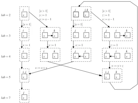
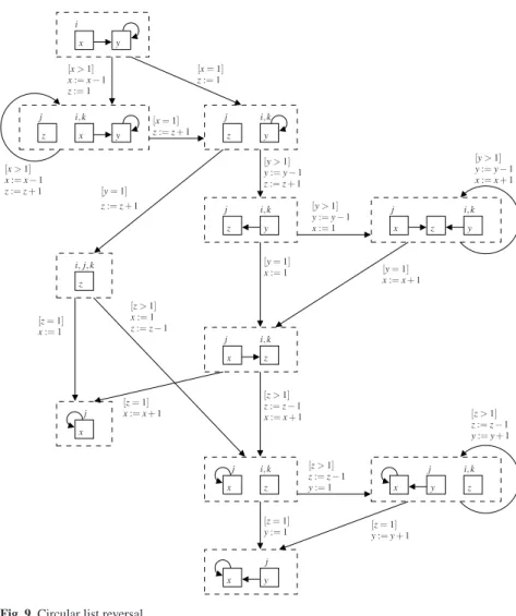
The List Reversal Example. Figure 8 shows the counter automaton bisimulating the list reversal program from Figure 2, started with a non-circular list pointed to by i as its input. The counter variable corresponding to each abstract node is depicted inside the node itself. Variables pointing to null are omitted. For each label of the program the corresponding control states are those reached after execution of the instruction at the label. The counter automaton for the same program working on a circular input is shown in Figure 9. For space reasons, only the control states where branching occurs are depicted.
4.2 Ordered Data Programs
In this section, we complete the definition of abstraction for programs with lists by introduc-ing an abstraction for heaps containintroduc-ing data from an ordered domain.D, /0. More precisely, we need to abstract the order relations that may occur inside a list segment and between two list segments.
Definition 5 Let H= .N, S,V, D0 be a concrete heap and H/∼ its quotient w.r.t. the RH
relation. If R ⊆ N × N is any relation on the set of nodes, we define the following for any [n], [m] ∈ N/∼: – oR([n]) iff ∀n 1, n2∈ [n] . (n1'= n2 ∧ n1RHn2) ⇒ n1R n2, – [n] /R f f [m] iff hd([n]) R hd([m]), – [n] /R f a[m] iff ∀n1∈ [m] . hd([n]) R n1, – [n] /R a f[m] iff ∀n1∈ [n] . n1R hd([n]), – [n] /R aa[m] iff ∀n1∈ [n] ∀n2∈ [m] . n1R n2.
1 Notice that a statement of the type u := w.next is used in a loop in this program, but in the derived
counter automaton, only one of the branches that arise from translating this statement stays in a loop—the other branch leads out of the loop.
x i x i x i x i, j x j y z x j i k x y j i, k j i y x j i y x i k x y x y i k y z x j i k i, j k y x [x = 1] x:= 1 [x = 1] x:= 1 y:= 1 x:= x − 1 y:= 1 [x > 1] x:= x − 1 z:= 1 [x > 1] z:= 1 y:= y + z lab= 2 lab= 3 lab= 7 lab= 4 lab= 5 x:= x + y
Fig. 8 Non-circular list reversal
For a concrete heap H= .N, S,V, D0, we define the relation c ⊆ N × N such that, for any n1, n2∈ N, n1c n2holds iff D(n1) / D(n2). Then, oc([n]) is true for a list segment [n] iff
all its elements are ordered w.r.t./. Similarly, [n] /c
=[m] holds for = ∈ { f f , f a, a f , aa} iff
the first (all) element(s) of[n] is (are) less than the first (all) element(s) of [m], respectively. Definition 6 An abstract heap is a tuple )H= .H, o, /f f, /f a, /a f, /aa0 where H = .N, S,V 0
is an abstract structure, o⊆ N is a unary ordering predicate, and /f f, f a,a f ,aa⊆ N × N are
bi-nary ordering predicates.
An abstract heap )H= .H, o, /f f, /f a, /a f, /aa0 sharing the same structure H = .N, S,V 0
as another abstract heap *H3= .H, o3, /3
f f, /3f a, /3a f, /3aa0 is said to be more precise,
de-noted as )H > *H3, if and only if we have o(n) ⇐ o3(n) and n /
=m⇐ n /3=m for all
= ∈ { f f , f a, a f , aa} and for each n, m ∈ N. Intuitively, the fact that a predicate does not hold for some abstract node indicates uncertainty w.r.t. the concrete ordering of the configuration. For instance, if o(n) does not hold, this means that in the concrete setting, n “represents” a list segment that may or may not be ordered.
Given a set S of abstract heaps sharing the same structure, we denote by8S the least upper bound, and by7S the greatest lower bound of S with respect to >. Note that 8 and 7 are undefined for sets of abstract heaps that have different structures. The domain of abstract heaps is denoted by. )H(PVar), >0. We say that an abstract heap is in normal form if the underlying abstract structure is in normal form. We write )Hn f(PVar) for the set of
abstract heaps in normal form.
Definition 7 Let H = .N, S,V, D0 be a concrete heap with data from an ordered domain .D, /0 and let H/∼= .N/∼, S/∼,V∼0 be its quotient. An abstract heap )H= .H, o, /f f, /f a
z j y i, k z y i, k j i x y i, k x y z j z i, j, k j i, k z y x i, k z x j j z i, k y x x j y x z i, k j x j [x > 1] x:= x − 1 z:= 1 z:= 1 [x = 1] z:= z + 1 [x = 1] [y > 1] z:= z + 1 x:= 1 y:= y − 1 [y > 1] x:= 1 [y = 1] [y = 1] x:= x + 1 x:= x + 1 y:= y − 1 [y > 1] [z > 1] z:= z − 1 x:= x + 1 [z > 1] z:= z − 1 y:= y + 1 y:= 1 z:= z − 1 [z > 1] y:= 1 [z = 1] [z = 1] y:= y + 1 y:= y − 1 [z > 1] x:= 1 z:= z − 1 x:= x + 1 [z = 1] [x > 1] x:= x − 1 z:= z + 1 [y = 1] z:= z + 1 [z = 1] x:= 1
Fig. 9 Circular list reversal
, /a f, /aa0 is said to be an abstraction of H based on H iff H is a structural abstraction of H
and for all[n], [m] ∈ N/∼and all= ∈ { f f , f a, a f , aa}:
– o(β([n])) ⇒ oc([n]) and
– β([n]) /=β([m]) ⇒ [n] /c=[m]
whereβ is the bijection linking H/∼and H in accordance with Definition 4.
For any concrete heap H∈H(PVar) and one of its structural abstractions H, we further define the most precise abstraction of H w.r.t. H asαH(H) = 7{ )H | )H is an abstraction
of H based on H}. For any abstract heap )H∈ )Hn f(PVar), we define the concretisation of
)
Hasγ( )H) = {H | αH(H) > )Hwhere H is the underlying abstract structure of )H}. Clearly, γ( )H1) ⊆ γ( )H2), if )H1> )H2, but the dual does not necessarily hold. Finally, the canonical
4.3 Counter Automata Semantics with Ordering Predicates
Taking ordering predicates o and/f f, f a,a f ,aainto account refines the notion of counter
au-tomata that we have so far introduced to model list manipulating programs. The counter automata defined in this section keep track of the ordering information, allowing one to ver-ify properties related to the ordering of lists, needed, e.g., to establish correctness of various sorting programs, such as InsertSort, BubbleSort, etc.
In order to achieve an enhanced precision of our abstract operational semantics without introducing too many different cases into it, we have designed our abstract state transformer function in two stages. The first stage yields the actual change of the predicates, and the second one is an operation of “saturation” whose goal is to add all the predicates that can be derived from the existing ones for a given abstract heap without changing the corresponding set of concrete heaps. Moreover, we assume to initially start from saturated abstract heaps.
In order to understand the intuition behind the saturation step, let us consider the case depicted in Figure 10. There are three abstract nodes n, m, and p in the figure such that n and m are ordered, and n≺a f pand p≺f amhold. Setting the v variable to null in this state
causes the nodes n and m to merge into n3which is ordered. In our abstract semantics, we introduce a rule for inferring o(n3) if n ≺
aamis known. In the example, we do not explicitly
have n≺aam, but n≺aamis a consequence of the transitivity of the order relation: n≺a f
p∧ p ≺f am⇒ n ≺aam. In order not to have to introduce the situation of n≺a fp∧ p ≺f am
as a separate case for when o(n3) can be inferred, we saturate the original state by adding
n≺aamto it before merging the nodes n and m.
u v w v:= null u o o o ≺a f ≺f a n m p n3
Fig. 10 An example of saturation
For the rest of this section, a counter automaton with ordering predicates is defined as Aa= .Qa, X,
a
−
→0 where the set of control states is now constructed as Qa= Lab×( )Hn f(PVar)
∪{Herr}) and the set of configurations asSa= Qa× (X → N), with the usual notation. In
addition to updating the abstract structure, the transition relation−→ has to also update thea ordering predicates.
4.3.1 Saturation
Let )H= .H, o, /f f, /f a, /a f, /aa0 be an abstract heap in normal form based on an abstract
structure H= .N, S,V 0, and let *H3be just like )Hexcept that all the components of the tuples
are primed. We define the saturation of )H to be the most precise abstract heap in normal form whose concretisation is the concretisation of )H. More precisely, *H0 is the saturation
of )H if and only if *H0= 7{*H3| γ( )H) = γ(*H3) ∧ )H=SH*3} where )H=S*H3holds for two
abstract heaps iff they are based on the same abstract structure. We say that )H is saturated if and only if )H= *H0.
Unfortunately, the above definitions do not allow one to effectively check that *H3is the
saturation of )Hfor arbitrary abstract heaps in normal form. The problem is that the setγ( )H) is infinite. To overcome this problem, we introduce “syntactical” saturation rules, given in
Weakening 1. n /aam⇒ n /a fm 2. n /aam⇒ n /f am 3. n /a fm⇒ n /f fm 4. n /f am⇒ n /f fm Reflexivity 9. n /f fn Transitivity 5. n /f fm∧ m /f f p⇒ n /f f p 6. n /a fm∧ m /f f p⇒ n /a f p 7. n /f fm∧ m /f ap⇒ n /f ap 8. n /a fm∧ m /f ap ⇒ n /aap Order 10. n /aan ⇒ o(n) 11. o(n) ⇒ n /f an
Fig. 11 Saturation rules
Figure 11. The closure of an abstract heap )Hin normal form w.r.t. the rules in Figure 11 is denoted as sat( )H). The saturation rules need to be applied with the following premises. Let ( )H, ν) be a configuration of the counter automaton and n an abstract node of )H.
– Ifν(xn) = 1, then it must be the case that o(n) and n /=n,= ∈ { f f , f a, a f , aa}, all hold
in )H. The reason is that list segments of size one are implicitly ordered, and the ordering relations are reflexive.
– Ifν(xn) = 2 and n /f an, then o(n) must also hold in )H. In a list segment of size two, if
the first element is less than the second, then the segment must be ordered.
The generated counter automaton tests, at each step, for each node n∈ N, whether xn∈ {1, 2}
and update the ordering predicates accordingly. Formal arguments for these updates are provided separately in Section 4.3.2. For the moment, let us carry on with the soundness proof for our abstraction.
Definition 8 Let )H= .H, o, /f f, /f a, /a f, /aa0 be an abstract heap in normal form based
on an abstract structure H= .N, S,V 0, let H = .N, S,V, D0 ∈ γ( )H) be a possible concreti-sation of )H, and letβ : N/∼∪ {⊥} → N ∪ {⊥} be the bijection from Definition 4. Then" is defined to be the strongest partial order on N satisfying the following for all n, m ∈ N, = ∈ { f f , f a, a f , aa}:
– o(n) ⇒ o!(β−1(n)) and
– n/=m⇒ β−1(n) /!= β−1(m).
Proposition 1 Let )H= .H, o, /f f, /f a, /a f, /aa0 be an abstract heap in normal form based
on an abstract structure H= .N, S,V 0, and let H = .N, S,V, D0 ∈ γ( )H) be a possible con-cretisation of )H. Letβ : N/∼∪ {⊥} → N ∪ {⊥} be the bijection from Definition 4, and let
sat( )H) be .H, osat, /sat
f f, /satf a, /sata f, /sataa0. We have that, for all n, m ∈ N, if n"m holds, then
one of the following holds:
1. n= hd([n]), m = hd([m]) and β([n]) /sat f f β([m]), 2. n= hd([n]), m ∈ tl([m]) and β([n]) /sat f a β([m]), 3. n∈ tl([n]), m = hd([m]) and β([n]) /sat a f β([m]), 4. n∈ tl([n]), m ∈ tl([m]) and either: (a) n R∗Hm andosat(β([n])) or
(b) not n R∗Hm andβ([n]) /sat aa β([m]).
Proof The proof is by induction on the length of the argument that one can use to show that n"mholds according to Definition 8, i.e., according to the number of times one uses the defining implications of Definition 8 to show that n"mholds. For the base case, we have:
– If n= hd([n]), m = hd([m]), we distinguish whether [n] = [m] or [n] '= [m]. In the former case, we haveβ([n]) /sat
f f β([n]) by the reflexivity rule 9. In the latter case, n"mholds
becauseβ([n]) /=β([m]) for = ∈ { f f , f a, a f , aa}, and we use the weakening rules 2, 3,
4 to obtainβ([n]) /sat f f β([m]).