A computer model for sound propagation around conical seamounts

A computer model for sound propagation around

conical seamounts

by

Jermie Eskenazi

Submitted to the Department of Ocean Engineering

in partial fulfillment of the requirements for the degree of

Master of Science

at the

MASSACHUSETTS INSTITUTE OF TECHNOLOGY

@Massachusetts

Institute

January 2001

of Technology, MMI. All rights reserved.

Author ...

Department of Ocean Engineering

January 19, 2001

Certified by...

Accepted by

Arthur B. Baggeroer

Ford Professor of Engineering,

Secretary of the Navy/Chief of Naval Operations

Chair for Ocean Sciences

Thesis Supervisor

Nicholas Patrikalakis

Kawasaki Professor of Engineering

Chairman, Departmental Committee on Graduate Students

A computer model for sound propagation around conical

seamounts

by

Jer6mie Eskenazi

Submitted to the Department of Ocean Engineering on January 19, 2001, in partial fulfillment of the

requirements for the degree of Master of Science

Abstract

This paper demonstrates a technique for computing the long-range sound pressure field around a penetrable conical seamount. The pressure field is generated by a harmonic point source. The seamount is positioned in a vertically stratified oceean. It is modeled as an outgrowth of the sediment layer covering the ocean bottom.

First, the seamount is decomposed into superposed rings of diameters increasing with the depth. Thus the problem reduces to a cylindrically layered system. Then, the method of normal modes is used to compute the sound pressure field in each layer. In order to maintain numerical stability, the Direct Global Matrix approach is used. The radial eigenfunctions are expressed as functions of normalized Hankel and Bessel functions, and the linear system that arise is organized in an unconditionally stable matrix.

The results show a perturbation zone behind the seamount. It is bounded by two lines going from the source and tangent to the ring that is at the depth of the source. The values of the sound pressure inside the perturbation zone can be higher or lower than the values outside of it, according to the dimensions of the seamount.

This work was supported by the United States Navy, Office of Naval Research, under contract N00014-99-1-0087.

Thesis Supervisor: Arthur B. Baggeroer Title: Ford Professor of Engineering,

Secretary of the Navy/Chief of Naval Operations Chair for Ocean Sciences

Acknowledgments

This thesis is written in memory of my grandfather Haim Levy and my grandmother Sarah Eskenazi.

First, I thank my mother and father for supporting, guiding and above all, loving me. I especially thank my sister whose kindness and humour spice up my life.

Second, I thank my advisor Arthur B. Baggeroer for giving me this research topic and the ideas necessary to explore it.

Thanks to all the students and staff of MIT's Ocean Engineering Acoustics Group for their help. Thanks to Peter Daly for solving my first computer problems. Thanks to Yi-san Lai for his extraordinary patience when answering my questions. Thanks to David Ricks of Science Applications International Corporation for explaining to me the ideas in his thesis.

Also, I thank the friends who supported my exploration of the United States the most: Tom Scharfeld and Ian Ingram.

Finally, I thank all of my friends and family in France, Israel, and Spain, who give my life pleasure and meaning.

Contents

1 Introduction

1.1 M otivation . . . . 1.2 Previous work . . . . 1.2.1 Experimental results . . . . 1.2.2 Theoretical approach of the problem

1.2.3 Direct Global Matrix approach . . .

1.3 Roadmap . . . . 2 The environment

2.1 The waveguide ... 2.1.1 The sea surface . . 2.1.2 The bottom ...

2.1.3 The sediment layer . . 2.1.4 The seawater . . . . . 2.2 The seamount . . . .

3 Analytical formulation

3.1 Taroukadis's approach to the p

3.1.1 The inner region . . . 3.1.2 The external region . .

3.2 Numerical treatment of loss me

3.3 Normalization of Hankel functi

3.3.1 Solution in the inner reg

12 . . . . 12 . . . . 1 2 . . . . 13 . . . . 13 . . . . 14 . . . . 16 19 roblem . . . . 19 . . . . 2 2 . . . . 24 chanisms . . . . 26 ons . . . . 27 ion . . . . 28 8 . . . . 8 . . . . 9 . . . . 9 . . . . 10 . . . . 10 . . . . 1 1

3.3.2 Solution in the external region . . . . 31

3.4 The source and boundary conditions . . . . 32

3.4.1 The boundary conditions. . . . . 33

3.4.2 The source condition . . . . 34

3.5 The matrices . . . . 36

3.5.1 Decoupling of the system. . . . . 36

3.5.2 Mapping of the matrices . . . . 37

4 Results 42 4.1 Discussion of the number of modes . . . . 42

4.1.1 Number of vertical modes . . . . 42

4.1.2 Number of circumferential modes . . . . 44

4.2 Special cases . . . . 46

4.2.1 Back scattering . . . . 46

4.2.2 No seamount in the waveguide . . . . 47

4.3 Cylinders . . . . 51

4.3.1 Validity domain of the results . . . . 51

4.3.2 Example of perturbation zone with a high sound pressure level 54 4.4 Decomposition of the seamount into several rings - Final results . . . 57

4.5 Conclusion . . . . 60

5 Conclusion 61 5.1 Sum m ary . . . . 61

5.2 Future work . . . . 62

A Nomenclature 63

B Computing technical details 65

List of Figures

The environment . . . . Temperature profile . . . . Sound speed profile . . . . The seamount . . . .

3-1 Eigenfunction for the 38th mode at r > R . . . .

3-2 Decomposition of the seamount into three rings - side view

3-3 Decomposition of the seamount into three rings - top view 3-4 Hankel and Bessel functions for p = 1 . . . .

3-5 Example of a matrix A, . . . .

4-1 Attenutation in function of modes, in m 1. . . . .

4-2 Pressure at the source as a function of circumferential order . 4-3 Back scattering 4-4 4-5 4-6 4-7 4-8 4-9 4-10 4-11 4-12 4-13

No seamount in the waveguide . . . . No seamount. p = 0 ... 100 . . . . No seamount. p = 0 ... 400 . . . . No seamount. p = 0 ... 1300 . . . . Cylinder of radius Rr = 5000 m . . . . Cylinder of radius R, = 5000 m. p = 0 ... 561 . . Cylinder of radius R, = 10 km. Depth = 1000 m

Cylinder of radius R, = 10 km. Depth = 500 m

Cylinder of radius R, = 10 km. Depth = 3000 m .

Decomposition of the seamount into 2 rings . . .

2-1 2-2 2-3 2-4 13 15 16 17 . . . . 21 22 . . . . 23 28 . . . . 41 . . . . 44 45 . . . . 4 6 . . . . 4 7 . . . . 4 9 . . . . 5 0 . . . . 5 0 . . . . 5 1 . . . . 5 3 . . . . 5 4 . . . . 5 6 . . . . 5 6 . . . . 5 7

Chapter 1

Introduction

This thesis describes my research on the long-range underwater acoustic field around a conical seamount generated by a harmonic point source.

Long-range underwater acoustics is a particularly challenging field since usual acoustic equations require special mathematical and computational treatments to produce accurate results far from the source.

1.1

Motivation

My work was supported by the United States Navy, Office of Naval Research. Its general goal is the improvment of our understanding of underwater sound propaga-tion.

A specific application of my research is the help on the detection of illegal

under-water nuclear testing.

International organizations, like the Comprehensive Test Ban Treaty Organization (CTBTO), monitor global environments to ensure the respect of treaties banning ex-periments on nuclear weapons. Underwater nuclear tests release large amounts of acoustic energy (frequency 1-100 Hz) into the water. Because sound energy in the ocean is guided by temperature and density variations through the so-called SOFAR channel, the signals from underwater explosions can travel many thousands of kilo-meters and still have amplitudes large enough to be detected by underwater acoustic

sensors (hydrophones). The CTBT specifies a network of six hydrophones stations and five T-phase stations (island-based seismograph stations that can detect an ocean acoustic wave when it converts to a seismic wave upon striking the ocean bottom near the island). The hydroacoustic monitoring network has few sensors because of the high efficiency of the propagation of signals into the ocean.

My research is part of understanding how low-frequency sound waves travel around

seamounts and thus determining if a seamount can screen the waves generated by an explosion.

1.2

Previous work

Acoustic perturbation by seamounts can be examined through experimentation and through theory. However, because of the complexity of the problem, both theories and experimental results that can be found in literature fail to provide clear views of the perturbation zones behind seamounts.

1.2.1

Experimental results

Nutile and Guthrie experimentally identified the acoustic shadowing by seamounts located north of the Hawaiian Ridge and explained it as the blockage of propagating rays by the seamounts [1].

More recently, Ebbeson and Turner measured the loss between a source and a multi-hydrophone receiving system over the Dickins Seamount in the Northeast Pa-cific Ocean [2]. Then Chapman and Ebbeson performed more measurements over the Dickins Seamount and concentrated on the study of the shadow zone that ap-pear behind it [3]. Jensen et al. compared theoretical predictions, obtained with a Parabolic equation model, with the experimental transmission-loss data collected by Chapman and Ebbeson [4]. The agreement between theory and experiment was seen to be excellent.

All the measurements of the perturbation of the sound behind a seamount have

" The data were always collected along a straight line going from the source and

through the center of the seamount. Therefore, the results are insufficient to describe the shape of the perturbation zone behind the seamount.

" Experimental results always show that the perturbation zone is a shadow zone,

i.e., a zone of lower sound pressure.

1.2.2

Theoretical approach of the problem

The effect of the seamount on long-range propagation can be qualitatively assessed from ray diagrams. Harrison derives analytical ray paths and shadow zone boundaries for some bottom topographies, including a seamount [5]. However, this method can not be a substitute for detailed analysis of intensity by normal mode theory.

Athanassoulis and Prospathopoulos present a normal mode solution for the three-dimensional problem of acoustic scattering from a nonpenetrable cylindrical island in shallow water [6]. Although their numerical simulations do not have the same dimensions as mine, their results about the number of azimuthal terms required to achieve numerical convergence as a function of the dimension of the environment will be useful to analyze the validity of my results (c.f. section 4.1.2).

The main inspiration for the modeling of the seamount and the normal mode solution exposed in this thesis comes from Taroukadis's work on the decomposition of the seamount into superposed rings [7]. Taroukadis's idea is to decompose the range-dependent environment into a cylindrically layered system of range-independent environments. However, this method can yield unstable equations and Taroukadis fails to get significant numerical results.

1.2.3

Direct Global Matrix approach

In order to obtain a stable system from Taroukadis's model, I use the Direct Global Matrix approach (DGM). DGM was developed for plane layered viscoelastic systems

by Schmidt and Jensen [8], and applied to spherically layered systems by Schmidt [9]

DGM method allows the production of an unconditionally stable linear system by preventing the underflow and overflow of the solutions and by minimizing the

propagation of errors.

1.3

Roadmap

Chapter Two, The environment, describes the ocean environment where the seamount is located.

Chapter Three, Analytical formulation, contains the analytical formulation of the problem.

Chapter Four, Results, describes and discusses the results.

Chapter Five, Conclusion, summarizes the results and offers suggestions for future work.

Appendix A contains the nomenclature followed in the mathematical

develop-ments.

Chapter 2

The environment

2.1

The waveguide

The seamount is located in an ocean modeled as a vertically stratified medium. The ocean is an acoustic waveguide limited above by the sea surface and below

by the sea floor. This waveguide can be modeled in many ways, according to what

aspect of the sound propagation we want to focus on [4], [11]. I consider a three-layered waveguide as shown in Figure 2-1.

The waveguide is made of a surface, a bottom, a sediment layer, and a water column.

2.1.1

The sea surface

I consider the sea surface as a perfectly free boundary, with a Dirichlet boundary

condition [12]. At the surface, the pressure becomes null:

p(surf ace) = 0. (2.1)

Above the surface, I model the atmosphere as a vacuum. Because the difference between acoustic impedances in the water and in the air is large, there is no need for a more sophisticated model of the atmosphere in the top half-space.

Figure 2-1: The environment z = 0 at surface

Atmosphere _{/ Pressure release boudary}

Sea water hE = 4000 Sediment layer h = 5000 Rigid bottom z axis

kilometers). Therefore I neglect surface scattering, which has significant effects only at short range.

2.1.2

The bottom

I assume that the bottom of the sediment layer is perfectly rigid. It verifies a Neumann boundary condition of the form

-- (bottom) _{= 0,}

dz (2.2)

which states that the normal component of the sediment particle velocity vanishes on the bottom.

2.1.3

The sediment layer

In the case of a three-dimensional propagation, an acoustic medium is characterized

I assume that the sediment layer is an isovelocity medium (i.e., the sound speed

remains constant at any depth and range) with the following characteristics:

Table 2.1: The sediment layer environment Top depth 4000 m

Bottom depth 5000 m

Sound speed 1600 m/s

Density 1100 kg/M

2.1.4

The seawater

In the seawater, I consider a constant density and a depth-dependent sound speed profile.

Table 2.2: The seawater environment Top depth 0 m

Bottom depth 4000 m Sound speed c(z)

Density 1000 kg/m

Measurements have provided an empirical function for the sound speed profile c

as a function of Temperature T, Salinity S, and depth z [13].

c =1448.96 + 4.951 T - 5.304 x 10-2 T2 _{+ 2.374 x}

10- T3 + 1.340 (S - 35) + 1.630 x 10-2 z + 1.675 x 10- 7 z2

- 1.025 x 10-2 T (S - 35) - 7.139 x 10 1 3 _{T z}3 _(2.3)

where T and S are functions of z.

tempera-ture profile in the open ocean [14]: T(z) in 'C is

(2.4)

T(z) = OOO0 ~10 z + 15 f or z

<

(h-OO) (1000 - z) + 5 for z > 1000m

where h is the depth of the sediment layer (h = 4000 m.) It produces a simple profile (Figure 2-2).

Figure 2-2: Temperature profile

500 1500 2500 3000 3500 0 5 10 15 Temperature ( C)

Again, I am interested in sound propagation at long range so I neglect temperature irregularities at the surface. The model does not take into account the temperature profile in the mixed layer (between 0 m and 100 m) where temperature varies greatly with the seasons.

The sound speed profile produced by such temperature and salinity profiles is shown in Figure 2-3. It forms a SOFAR duct at 1000 meters below the surface. The existence of a SOFAR duct allows long-range sound propagation since rays of sound launched above a certain angle will travel without bouncing on the waveguide boundaries and thus propagate with a lower transmission loss [15]. For this reason, I

n

A nn

--Figure 2-3: Sound speed profile

1low - - - - -SOFAR AXIS - - -

-- 1500-2000 - S2500- 3500-4000 4500 5000 1485 1490 1495 1500 1505 1510 1515 1520 1525 1530 Sound Speed (m/s)

usually position my source at depth zo = 1000 m.

2.2

The seamount

Taroukadis's model [7] is the benchmark for my research. Therefore, for the whole thesis, I will use the same notation as he does. The seamount in the ocean waveguide is under an acoustic wave generated by a point source, as depicted in Figure 2-4. It is modeled as an outgrowth of the sediment layer that covers the ocean bottom. I use the cylindrical-polar coordinates T = (r, 0, z) with the z-axis oriented downward. The variables used to describe the environment follow:

Figure 2-4: The seamount 0 R 0i source (RO,0, zo) inner region r external region n hE Ih z

h = depth of the sea bottom

hE = depth of the sediment layer

'r = radius of the base of the seamount Pi = density of water

P2 = density of the sediment layer

= unit normal vector outside the sediment layer

Som = surface of the seamount

Sb = surface of the sediment layer

(RD, 0, zo) = coordinates of the source

k = wavenumber = w/c(z)

The top of the seamount is 50 meters below the sea surface. The radius of the seamount R, is equal to 10 kilometers.

For all numerical applications, I consider the source as a harmonic point source of frequency

f

The waveguide can be divided into two regions:

* an inner region for r < R[, where the seamount is located,

* an external region for r > RI.

We will see in chapter 3 how the waveguide can be further decomposed in order to solve the problem.

Chapter 3

Analytical formulation

Solving long-range sound propagation problems poses important mathematical

chal-lenges. Indeed, before any computation can be performed, it is important to find a way to handle the unstable equations that arise. Far from being restricted to my particular subject, the mathematical method described in this thesis can easily be applied to most acoustics problems involving multiple layers.

In the first part of this chapter, I will follow Taroukadis's work [7] for the analytical formulation of the pressure field. In the second part, I will provide details about the numerical treatment of loss mechanisms. In the third part, I will solve the equations obtained by Taroukadis using Schmidt and Jensen's normalization of the Hankel and Bessel functions [4]. Finally, in the fourth part, I will describe the linear system to solve and I will discuss the numerical stability of the method.

3.1

Taroukadis's approach to the problem

The benchmark for my research is the work of Taroukadis on sound propagation around conical seamounts [7]. Therefore, this subsection is just an application of Taroukadis's approach to the problem.

the inhomogeneous wave equation governing the pressure field p is given by 02_{p l} Ip 1 2 2p 1 dp ip 2 1 + -- -+ +

{k(r,

There are many methods to solve Helmoltz equation. Among them, the normal modes theory is the most appropriate to solve problems in horizontally stratified media.

Using the method of normal modes, the solution of the wave equation is expressed in terms of radial and depth eigenfunctions:

00 00

p(r, z, #) = 1 1 Rmn(r)Un(z) 0 m(#),

n=1 m=O

with V#m being a basis of sine functions, namely,

(3.2)

'bm(o) = em sin(m), m = 0,1, ...

where em is defined as follow

em = /,

-,

M = 0 M f 0

The circumferential eigenfunctions Om are orthogonal:

Ir

The depth eigenfunctions Un satisfy the eigenvalue equation

d p(z) d dz

]

where kn are discrete values of the horizontal wavenumber (or radial wavenumber)

(3.3)

associated with eigenfunctions U.

The depth eigenfunctions U, can be scaled arbitrarily. I scale them so the norm

C, is unity, so the orthonormality of U, with respect to the weighting function 1

yields h

I

Each mode has a non-vanishing field in the bottom. This is illustrated in figure 3-1 where the eigenfunction for the 38th mode is shown, as an example, in both the water column and the sediment layer for r > RI. We will see in section 4.1.1, Number of

Figure 3-1: Eigenfunction for the 38th mode at r > R1

-0.05 -0.04 -0.03 -0.02 -0.01 (

U 3 (Z)

0.01 0.02 0.03 0.04 0.05

vertical modes, how this behavior allows us to

for the convergence of the double series 3.2.

lower the number of modes required

At this point, Taroukadis defines an inner region for z <

IRr

...-3.1.1

The inner region

The inner region, indicated by superscript I, contains no real source. Therefore, the wave equation to solve is the homogeneous Helmholtz equation, given by

a2p1 1 dp Op'

+Z2 _{p(z) dz Oz} +

{

2_{p 0.}

In this region, Taroukadis models the seamount as a superposition of I vertical rings of radii R,. An example of the decomposition of the seamount into three rings is depicted in figures 3-2 and 3-3.

Figure 3-2: Decomposition of the seamount into three rings - side view

Re: source (R_0, 0, z ) inner region 0 r external region Z

Obviously, the more the rings taken in the decomposition, the better the approx-imation.

For each ring i, it is thus possible to write the pressure field pf as

pf (rz,#)

=

Figure 3-3: Decomposition of the seamount into three rings - top view

external region

R3= R,

4ource

Inner region

Substituting equation 3.9 in equation 3.8 gives

U (z)m(#) 0= =0 + Rf,(r)V)m(q() d2_{R(r) 1 dRmn (r} dr2 _{r dr} d2_U|I(z) dz2 1 dU| (z) pdz dz m2 r2 Rm(r) (k')2U[I(z)

Inserting equation 3.6, multiplying by -yU'l,,(z), integrating from 0 to h and using the orthonormality of the depth eigenfunctions 3.7, it is found that

1 dRfi(r) 2m 2

+ + (k,,)2 Rjg(r) =0.

r dr r2 (3.11)

Multiplying by @/(#), integrating from -7r to 7r and using the orthogonality of the

-= _{0. (3.10)}

[d2R,

circumferential eigenfunctions 3.5, it follows that

Rd(r) + [(k )2RI()

)2

dr r rdr 14" [v~

for rei K r < R, and i = 1, 2,... I, where kf are the discrete values of the horizontal

wavenumber associated with the eigenfunctions U (z) of the ith ring.

Equation 3.12 is a Bessel equation of order p for the function R,,'(r) [16]. Taroukadis solves this equation with Hankel functions:

R2(r) = E (k ,.r) + F' Hj (kr). (3.13)

where E and FV are some coefficients to be determined with the boundary

condi-tions.

This solution is numerically unstable because of the behavior of Hankel func-tions for short ranges and high circumferential orders: if p. is greater than kvr, then

H1 (kyr) and H (kvr) approach infinity very quickly. Therefore, this method

re-quires special numerical efforts to maintain numerical stability for large values of P. In section 3.3, I will demonstrate how numerical instability can be avoided using Schmidt's and Jensen's normalization of the Hankel functions.

3.1.2

The external region

In the external region, indicated by superscript E, the source must be taken into account. Therefore the equation to solve is the inhomogeneous wave equation 3.1.

Equation 3.2 can be re-written as

00 00

pE(r, z, = R.) (U ( (3.14)

n=1 m=O

The general method used in the calculus of equations 3.10, 3.11 and 3.12 still holds true, but the effects of the source must now be considered.

Substituting equation 3.14 in equation 3.1 gives d2_R.. (r) dr2 d2U (z) dz2 1 dR E(r) r dr r2 - nRE (r)\ 1 dpdU(z) k2UE(Z] pdz dz + (k, n ) 1 = -- J(r - Ro)6(q)J(z - zo). r (3.15)

Plugging equation 3.6, multiplying by 1 U (z), integrating from 0 to h and using the orthonormality of the depth eigenfunctions 3.7 yields

[d

{

Multiplying by i/($), integrating from -7r to 7r and taking into account the orthog-onality of the circumferential eigenfunctions 3.5, it follows that

+ d R ,(r) r dr 01,(0) U (zo)

I

where kE are the discrete values of the horizontal wavenumber associated with the eigenfunctions UE (z) of the external field.

Again, equation 3.17 is a Bessel equation of order p for the function RE()

As for the internal field, Taroukadis solves Bessel equation with Hankel functions of the first and second kind:

(3.18) R E() ,01 (0) UVE (ZO) 1"1 for R < r < R, and R(r) V),(0) UE (ZO) (3.19) EUE n(Z)m()= n1 m=O + Rmn(r) QO) R(r)

1

(k.

for r > RO.

As I indicate in section 3.1.1, these solutions are unstable for large values of y.

I use different solutions in section 3.3.

3.2

Numerical treatment of loss mechanisms

Complex wavenumber

We must take volumetric absortion into account in the computation of the sound pressure field. This is easily achived by manifesting the loss with a complex sound speed: c(z) = co(z) + ici(z), where co corresponds to the unperturbed sound speed

profile. The wavenumber then becomes k2_{(z) = k2(z) + ik2(z) = , that is,}

k2 2 W 2 _+2iW2 COC[ (3.20)

c2 + c [c c]2 (3.

Computation of the imaginary part of the sound speed

Equations for material absorption in the water column are summarized by Urick [19].

If we assume that c2 < c2, then ci ~ 2c2 where a is the absorption coefficient in

nepers/m.

A simplified expression of the absorption coefficient in the seawater as a function

of the frequency f in kHz is

1 0.11f2 44f2 _[nprm]

a = 1 3.3 x 10-3+ 1 + f2 + 44f2_ + 3 x 10-4f2 [nepers/m.

1000 x 8.68589 + f2 4100+f2

(3.21)

Thus in the water, a = 3.8550 x 10-7 nepers/m for f = .02 kHz. The equivalent in

dB/A is a = 2.5113 x 10-4 dB/A.

In the sediment layer, the absorption coefficient as a function of f in kHz is 1

Thus in the sediment layer, a = 2.3026 x 104 nepers/m for f = 20 Hz. The equivalent in dB/A is a = 0.1500 dB/A.

Computation of the imaginary part of the radial wavenumber

The introduction of a complex part to the wavenumber naturally affects the radial

wavenumber, which becomes kn= kO + iknl.

For the details of the computation of the imaginary part of the radial wavenumber

kni, refer to Jensen et al. [4]. It is found that

h k 2(Z)Ul)

kai = dz. (3.23)

Sp(z)

Thus the radial wavenumber, which appears as an argument of the Hankel func-tions, is a complex number. Therefore, the solutions of Bessel equations 3.12 and 3.17 will decrease as the range r increases. This behavior represents the natural attenua-tion of sound as a funcattenua-tion of range.

3.3

Normalization of Hankel functions

Problems of unstability that arise for large circumferential orders can be avoided by using the direct global matrix approach (DGM). DGM was developed for plane layered viscoelastic systems by Schmidt and Jensen [8], and applied to spherically layered systems by Schmidt [9] and to cylindrically layered systems by Ricks and

Schmidt [10].

In our problem, since the seamount is decomposed into rings, the model reduces to a cylindrically layered system. (Cylindrical layers are visible in the top view of the seamount 3-3.) Therefore, DGM is well suited for the problem.

The first idea in DGM is the normalization of Hankel and Bessel functions. Bessel equation in the inner region (3.112) and in the external region (3.17) must be solved

3.3.1

Solution in the inner region

General solutions to Bessel equation

Theoretically, solutions to Bessel equation in the inner region (3.12) can be any linear combination of two of the functions J,(x), Y (x), H( (x), and H 2)(x) [17]. However, as explained by Ricks [18], only one pair can be chosen to avoid loss of distinction between asymptotic behaviors.

For

lxi

>

H( 1)(x) ~ #2/-(7rx) e'(x-,ox/2-7r/4)

H I2)(x) ~2J() ~ 2,x 2(r)ei(x-jAr/2-7r/4)

The loss of distinction between the functions J,, Y,, and H 2) is illustrated in figure

3-4, where the functions of order p = 1 are drawn along the axis {x = a + ib}b.=.

Figure 3-4: Hankel and Bessel functions for p = 1

2 I H (2H 2Y 0.5 0 -0.5 -1.5 _H(1) -2- -2.5--3x'

And for |p| > jxj,

J,(x) (x/2)14/ F(p + 1)

Y,(x) ~ -iH,(')(x) ~- i H, .2(x) ~ -(1/7r) F(p)(x/2)-1

Therefore, the only pair of function that preserves linear independence for both

jxI > p and IpI > xj is Hi' (x) and J,L(x).

Normalization

I solve Bessel equation 3.12 with the following set of functions:

S

H (k[ r)

R,'J(rW) = E( ' + F,,J, (k,,r) H4' (kivR for r

E

In the first ring i = 1, the sound pressure must be finite for r = 0. So the solution

keeps only the Bessel function J,:

R4'J(r) = A1,J, (kf,,r) H(' (k,,R1) for r E [0; R1]. (3.25)

Note that solution 3.25 is part of the set of solutions 3.24 if we consider Eu1 = 0 and

a= Ali.

These normalized solutions provide numerical stability by doing two things:

1. For p

>Ik,,rl,

Ik[,rI

>

there is evanescence across layers.

I explain these two points in more details below.

To illustrate the first point, let us examine a numerical example. We will see in section 4.1.2, Number of circumferential modes, that p can take values as high as 2600. For this numerical example, I take parameters that produce numbers that

normalization, we would have

HJ000 (kfO, 1Ri0) -3.3610 x 10+25 + i x -8.0828 x 10+259 and J1ooo (kf0,1Rio) = 4.3431 x 10-26 + i x 1.8064 x 10-266.

The overflow of the Hankel function and the underflow of the Bessel function lead to unstability in the system since computers can not multiply or divide such num-bers without a significant loss of precision. The same numerical coefficients with normalization are

H ]5M (kf, Rio)

H00

(k1

₎

and J1000 (kf0,1Rio) HIJ)o (kf0 0,1Rio) = 3.4828 x 10-10 + i x -3.5105 x 10-4.

Thus, the number obtained are far enough from the computational limits of the computers.

To better understand the second point, let us consider as an example the case where lk,,rl

>

>

then close to the boundary r = R, between cylinder i and (i + 1),

H (k r )

H< J (k,,r) H([) (k!ri) (3.26)

This means that the effect of boundary r = R, does not propagate far from it.

The same can be observed at boundary r = R,_1. If Ik[,r I

>

>

HM (k! r)

H I

(k,

(k,,r)

(k

Again, in case of evanescence across boundaries, the effect of boundary r = R,_1 does not propagate.

These solutions respect the physical idea that the effect of a boundary should not be perceveid far from it. In case of evanescence i.e., if the imaginary part of the wavenumber is great compared to 1, this reduces the propagation of errors from one boundary to an other and therefore maintains numerical stability.

In section 3.5 and figure 3-5, we will see how the final mapping of the system can implement the decoupling described above.

3.3.2

Solution in the external

region-Equation 3.17 is solved similarily to equation 3.12. For r E [RI; Ro],

H(k Er)

RHi(rl = B C,,J, (kr) H ' (k? Ro)] V$',(0) U (zo). (3.28)

For r > RO, the sound pressure must go as H,') (kir) to satisfy the radiation

condition at infinity [16]. Therefore, the solution for r > RO is

RE(r) = Dill, r () U ( zo). (3.29)

HM (k ERO) 04o Z

As explained in section 3.3.1, these solutions provides numerical stability since they reduce the effects of boundaries into each other. To illustrate this behavior, let

us take Ik'r

>

Ht~ (k~r)< J) (kEr) H(') (kERo). _(3.30)

H(' (kIR,) M V

And for r ~ RO,

HI(l

(k

V >J,

(

(k

Thus, as in the inner region, these solution maintains numerical stability by:

2. Reducing the propagation of errors in case of evanescence across boundaries.

3.4

The source and boundary conditions

By replacing solutions 3.24, 3.25, 3.28 and 3.29 into the expression of the pressure 3.2,

we have:

pf (r, z, #) = _AmJm

_(k,=r)

_(k,,R)

n=1 m=O

for r E [O; Ri],

(3.32) 000 cc H' ( H() (k r) E= = Hm")

(kj,

for r C [RI; RO], and

Hm) (kEr)

PE (r, z, )= Dmn H UE (zo) Om(0) UE (z) 4'm(0)

p1 m=O HY(k R0 )

(3.35)

for r > RO.

Note that equations 3.32, 3.33 and 3.34 can be summarized in a single equa-tion. If we define E =Amn, F

-

-Cmn Un (zo) Vbm(0), 1P1+1E = =Eand R1~ RO, we obtain an expression of the pressure

(3.33) Ui,(Z) OM (#)

U(zo Em0U (Z) )

similar to equation 3.33 that is true for all r E [0; Ro]:

pi(r, z,/ = E (kr + FmnJm (ki,nr) H() (kinRi) U(z)

'm(q)-n=1 m=o HZ) Ui- (kVn~ _

(3.36)

To solve the problem, we need to approximate the solutions by taking a finite number of vertical modes n and circumferential modes m in the expression of the pressure field. If we take N vertical modes and M + 1 circumferential modes, then we have 2 x N x (I+1) x (M +1) unknown coefficients A, E, F, C, and D. We need the same number of source and boundary conditions to be able to solve the problem.

3.4.1

The boundary conditions

Continuity of pressure

At boundary r = 1I, the continuity of pressure yields

pj(R , z, #) = pi+1(Ri, z, #) for i = 1, 2, . .. ,J. (3.37)

This means that the acoustic pressure must be continuous between the rings.

We replace the pressure by its series expression 3.36 and we limit the calculus to the first N vertical modes and M+1 circumferential modes. Multiplying equation 3.37

by elcos#, integrating from --w to 7r and using the orthogonality of the circumferential

eigenfunctions, we obtain a set of M + 1 equations,

[E n H') (knJ4) F n J (kAn R) H(') (k

1

)

N

E ni + F JA (+,nl ) H() (kj+1,n1 '+1)] Ui,n(Z). 3.8

orthonormality of the vertical eigenfunctions, we get a set of N x (M + 1) equations HE' (k ,RJ?) Ea + F JA (k1,vRi ) H l (k ,-R1) = N N E +1_Z.'+1 _{+ EF Jy (k} 1 ,nJZ%) H(1 (kj+1,1R+1) Zg'.+1. n=1 n=1

Continuity of the normal component of fluid particle velocity

The continuity of the normal component of fluid particle velocity at interface r = produces (3.39) 1 pi pi Or 1 OPi+1( ,Z7 Pi+1 Or for i = 1, 2, ... , I.

By doing the same operations as between equations 3.37 and 3.39, we obtain

+ F,, ki,v-- (ki,vRz) H( ) (kj,VR ) = dr E +nki1, _{(kj+1,vR%) A)4+} N + +kV (k+ 1,nT) Hn (k1+1,nRi+1) A Z$,+1. n=1 (3.41)

For each interface, there are N x (M + 1) equations 3.39 and N x (M + 1) equa-tions 3.41. The continuity condiequa-tions at the boundaries thus yield 2 x N x I x (M +1)

equations.

3.4.2

The source condition

If we multiply equation 3.17 by r, we obtain a Sturm-Liouville equation of the form

sV2_u

+ VsVu - qu = -pF (3.42)

(3.40)

E'~i~ dr '

E R(r)

where s(r) = r and u(r) = ,-(O) U (zo). Equation 3.42 implies two continuity

condi-tions at r = RO [20]: u(R+) = u(R-) (3.43) and du dr du 1 dr = s(Ro) (3.44)

Replacing R',(r) by its expressions 3.28 and 3.29, equation 3.43 becomes

HBt (kvR0) +

C

B ,yL1 (kq R+C ,Jy(kvR₀)H f')(kvR₀) =D,

Hffyl (kvR,) 1 (3.45)

and equation 3.44 becomes

Sdr dHl 1(kvRo)

H (kv R ) 1

(3.46)

To compute the derivatives of J and H, we use the recurrent relation

C'(z) = -CA+ 1(z) + -CA(z)_z (3.47)

where C denotes J or H [17].

Solving the set of equations 3.45 and 3.46, we find that CL, can be separated and expressed as a function of the Wronskian of J, and H,:

C-C W=

-1

kvRo W [Hjj(kvRo); Jgj(kvRo)]'

A trivial calculation gives W [H ,(kRo); J,(kRo)] = _{Crk =Ro}"i, and thus

-nr CV

₂

We can also compute B,, as a function of D,, and C,

Blv = Dtv HF) (_kR - C14 J, (kRo)

H'

HA (kVRO)

Thus, at the interface r = RO, we have a total of 2 x N x (M + 1) equations 3.49

and 3.50. With equations 3.39 and 3.41, we have a total of 2 x N x (I+1) x (M +1) source and boundary conditions, for the same number of unknown. Therefore, the linear problem can be solved.

As we can see in equation 3.50, B,, and D,, are directly related since we know the value of C,,. So in order to decrease the dimension of the system, we can exclude the unknowns D,, and equations 3.50 of the system. The dimension of the system then reduces to N x (21 + 1) x (M + 1).

3.5

The matrices

Equations 3.39, 3.41 and 3.49 form a linear system for the unknowns A, E, F, and

C. Therefore, they can be put on the form

A.X = B (3.51)

A is a matrix of dimension [N x (21 + 1) x (M + 1)]2 and 13 are vectors of dimension

N x (21 + 1) x (M + 1). X is the vector of the unknowns and B is the vector of the

forcing terms due to the presence of the source.

3.5.1

Decoupling of the system

We can see that the system is uncoupled among circumferential orders jt or m.

There-fore, it can be split into M + 1 sub-systems of dimension N x (21 + 1). For each

circumferential order p = 0,1,... , M, we need to solve a system of the form

A, are matrices of dimension [N x (21+1)]2. X, are the vectors of the unknowns

AA, E,,, F,,, and C,, for v = 1, 2, ... , N and p fixed.

3.5.2

Mapping of the matrices

For a given p, I take X, as follow:

[Ap,N] E ,N F1,1 XI = (3.53) F,11_ iE[2;N] [B,N] C,N

Therefore matrix

A,

The lines are described below.

iE[2;N] pN LI

L%

[i+J

' =, {J(k1,R1)H,,(k1.R1)} -v-1 N-v

(

2Ni-3N~v- 1 H A(kjvRi_(H4kv,,)N-I 1) (JA(kjvRi)HA(kjvI)) N-vN

(-Z

N N 2N(I-1) (3.57) L\-

=[

Q

-ki+ 1,V -- (ki+14R )HA (ki+l,vP4+1) AZn v+l

d=1,.., 2N(I-1) N 1 _{= [ OO} 2N1I-v-1 1 O

..

BA is a simple vector containing zeros and values of C,v that we calculated in

(3.55) k1v H kivRi_) N-1 N-v ] (3.58) (3.59) . kivd (kjIRi)HA(kjv Rt)

equation 3.49:

0

B,= 0 (3.60)

-i7r

2

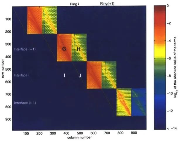
As an example of the form of the matrices obtained, Figure 3-5 shows matrix

Ai

logarithm of the absolute value of the dimensionless terms of the matrix. Except for the first and last blocks in the diagonal, the matrix is diagonal with blocks of the form of G, H, I and J (c.f. Figure 3-5). G is made of the terms

(-Zi+1) Nand -ki+ d

9(ki+,v ) AZi)i+1 Znvu n=1,..., N + ,vnv+,~

4(kj~~vRn=1, ... ,N

H is composed of

(-J (kj+1,v1 )Hjj(ki+1,vlz+1) Zni'v+1) n=1, ... ,N

and

(-k+,v

r _/n=1,...,N

I is a diagonal line of the terms

HO(kivR ) an i T-(kjvR-)

and k Hk~

HjA(kivR _1) " HjA(kjvRz_1) and J is a diagonal line of the terms

Figure 3-5: Example of a matrix A,,: Matrix A1 for a decomposition of the seamount into 4 rings 0 -2 -4 -C -10 -62 -8 .2 -102o < -14 100 200 300 400 500 600 700 800 U0U column number E e

In this example, the imaginary part of the wavenumber is too small to consider that there is enough evanescence to reach the conditions of inequalities 3.26 and 3.27 in section 3.3.1. If there were a stronger evanescence, the values in block I would have been less than the values in block J. Thus, because the values in G are greater than the values in H, all the blocks of highest values would have been located along the diagonal of the matrix, making the solution more stable.

However, this is not the case here: The evanescent condition Im(ki)

>

Chapter 4

Results

I recall that, for all computations, I took f = 20 Hz.

4.1

Discussion of the number of modes

In order to compute the pressure, we must find the modes for which there is conver-gence of the double series 3.2.

4.1.1

Number of vertical modes

To compute the vertical eigenfunctions in the waveguide, I used the Kraken Normal

Mode Program [21]. The maximum number of modes in the waveguide increases with

the depths of the rings. The maximum number of modes in the region of the inner ring (r < R1) is 125 and the maximum number of modes in the region outside the seamount (r > Ro) is 132. Therefore, the maximum number of modes that I can

consider is 125.

Two different minimum mode numbers are required in the problems:

* The minimum number of modes needed to fill the matrices A, and solve the linear systems AA.X, = B, (3.52),

* The minimum number of modes needed to compute the double series 3.2 with enough precision.

Number of vertical modes in the matrix

In order to compute the unknowns E,, and F,, we need to fill the matrices A, and to solve the corresponding linear systems. The more vertical modes N we include in the computation, the more accurate the results. I noticed that the convergence of the vector of unknowns X,, as a function of the number of modes is rather slow: It occurs only after the 110th mode. Therefore, I take 110 modes into account to fill the matrix and solve the linear systems 3.52.

Number of vertical modes in the double series

In order to reduce the dimension of the system (and therefore reduce the time of the computation), we need to determine the minimum number of vertical modes required to achieve computation of the double series 3.2 with enough accuracy. The double series 3.2 converges quickly when the vertical eigenfunctions hit the sediment layer; that is, when the attenuation becomes strong enough to cancel propagation. Thus, there exist a vertical mode N for which

N mo

P('r, Z, 4) ~ 1 Rmnr)UnW)Om (0). (4.1)

n=1 m=O

This happens when the imaginary part of the wavenumber is great enough: if Im(kf,,r)I

>

As an example, figure 4-1 shows Im(ki,,) as a function of modes for a decompo-sition of the seamount into 4 rings.

The greater the ring number, the deeper the sea bottom. Therefore, when the ring number i increases, the mode number N at which the loss becomes significant increases. Thus, the minimum mode to take into account is the mode for which there is strong attenuation in the region r > RI, where the sea floor is the deepest. From

Figure 4-1: Imaginary part of the radial wavenumber in function of modes, in m-1 5r 4.5 4 3.51 3 2.5 E 2 1.51 1 0.51 x 10-4 ji Ring 1 Ring 2 Ring 3 SRing 4 r R 0 _N 3 20_N N2 N3 4 N 40 N _{Mode number}60

number of rings so the maximum number of vertical modes taken into account in the double series remains 35 for other computations with different numbers of rings.

4.1.2

Number of circumferential modes

To determine the maximum circumferential order M to take into account in the com-putation of the pressure, I compute the pressure for fixed circumferential orders:

N

p,(r, z, #) = [ Ryn(r)Un(z)@,(#).

n=1

(4.2)

Figure 4-2 is an example of the results obtained at the position of the source, N = 125. In this example, p,, becomes negligible after the

C _{80 100 120}

-Figure 4-2: Pressure at the source as a function of circumferential order -G5 -10 --15 -~ -20-a. 0-25 -0 -30 - -35- -40--45 1-0 500 1000 1500 2000 2500 3000 Circumferential order

2600th circumferential order. There are similar results for all other points in the

environment, so considering M = 2600 for computing the pressure at every range and depth produces precise results.

Athanassoulis and Prospathopoulos studied the minimum number of circumferen-tial orders M required to achieve numerical convergence as a function of the dimension of the problem, in the case of a cylindrical island [6]. They found that M increases proportionally to kRj. They studied some environments for which kRf E [4; 84] and determined M E [20; 200].

Our problem is larger since kR1 = 838 for R, = 10 km, but I still find that the value of M increases with the dimensions of the problem. For example, we would need to take M = 5400 for a seamount of base radius R, = 15 km. However, I did not study seamounts with base radius greater than 10 km because they would have been physically unrealistic.

4.2

Special cases

In order necessary

to check the validity of both the theory and my computer code, it was to apply them to particular well-known cases.

4.2.1

Back scattering

Figure 4-3: Back scattering

E, C Ca U: 250 -500 -450 -400 -350 -300 -250 -200 -150 -100 -50 0 Range (m)

Parameters: I = 1. Ri = 50 m. Depth = 1000 m. Source at (-250 m, 0, 1000 m).

When the sound field hits the seamount, a pencil of sound is beamed backward and its anglewidth is proportional to '. Therefore, if we take R1 small enough, we can observe the back scattering of the sound. This is illustrated in figure 4-3, in a case where the seamount is reduced to a cylinder of diameter R, = 50 m. The source is

positioned at RO = -250 m and the receivers are at the depth of the source (1000 m). 48 52 56 9 0 C 0 60 -64 68 72 76 ... ... I

The results are expressed in terms of transmission loss, defined as

TL = -20 logio , (4.3)

Pref

where Pref is a pressure reference: pref = 1 Pa.

The sound field looks perturbed between the source and the cylinder, which proves that the model is precise enough to compute the effects of back scattering. In later examples, I use a much greater R1, so back scattering becomes too small to be ob-served.

4.2.2

No seamount in the waveguide

Figure 4-4: No seamount in the waveguide

x10 5 80 90 -0.8 ---0.6 -100 ilyon AO" -0.4 110 0 .-0.2 E 0 120 ) Cc E 0.2 A 130 0.4

_J//

Figure 4-4 shows the results obtained when the seamount is a small cylinder of radius 50 cm. A black dot indicates the position of the cylinder.

The cylinder is too small compared to the wavelength to have a noticeable effect on the computation of the sound propagation. Therefore, this case is equivalent to the case where there is no seamount in the waveguide.

In figure 4-4, we can notice some perturbation zones, indicated by arrows. They are only due to the precision of the grid: the more points in the grid, the less visible these "perturbations." Because the time of the numerical simulation increases with the precision of the grid, it has to be limited. I am using 600 points in the grid, which is the limit precision for which I can obtain results in a reasonable amount of time.

In cylindrical coordinates, the spreading loss between the source and a point

(r, 0, z) is H = 10 x log ' where ref = 1 m. In the case of figure 4-4, the right-hand

limit of the region under consideration is at r = 200 km, so H should be in the order of 50 dB there. The results show the transmission loss varying from about 80 dB at the source to 125 dB at 200 km far from the source, which corresponds to H ~_ 45 dB. Thus the cylindrical spreading loss is within the order of the theoretical predictions. Moreover, these results are close to those obtained for similar problems [4].

Filling of the environment as a function of circumferential orders

We can notice the way the sound is computed as a function of circumferential orders

by comparing figures 4-5, 4-6, and 4-7. Figure 4-5 shows the results for p varying from 0 to 100. Figure 4-6 shows the results for g varying from 0 to 400. Figure 4-7 shows the results for p varying from 0 to 1300. As p increases, the computation produces results that fill the environment starting from axis q = 0 and cylindrically spreading

toward axes

#=

Figure 4-5: No seamount. p = 0 ... 100 x 1P -0.1 -0.4 cc ( U 100 110 120 $ 130 -5 10 Range (m) 15 20 x104 140 150 10

Parameters: I = 1. R1 = .5 m. Depth = 1000 m. Source at (-3000 m, 0, 1000 m).

We can see that the results inside the zones of high sound pressure level near axis

= 0 are identical to final results. In other words, the computation for circumferential

orders greater than a given Pi have little effect on the results obtained in the zone of high sound pressure level for p varying between 0 and p1.

Figure 4-6: No seamount. p = 0 ... 400 x 10 ₈₀ -1 90 -0.8 -0.6 100 -0.4 110 11 1 i120 Cc E 0.2A 130 0.4 0.6 140 0.8 _ISO 1 160 0 5 10 15 Range (m) x104

Parameters: I = 1. Ri = .5 m. Depth = 1000 m. Source at (-3000 m, 0, 1000 i).

Figure 4-7: No seamount. p = 0 ... 1300 80 -0.8 -0.6 100 -0.4 110 -0.2 p 0 120-0.213 150 160 0 5 10 15 20 Range (m) x10 4

4.3

Cylinders

The simplest case is the modeling of the seamount into one cylinder of radius equal to the base radius of the seamount. Of course, this case is not physically realistic, but it helps to determine the validity domain of the code.

4.3.1

Validity domain of the results

Figure 4-8 shows the results obtained for a cylinder of radius R = 5000 m. Figure 4-8: Cylinder of radius R1 = 5000 m

x 105 ₈₀ 90 -0.8 -t n -0.6 -100 -0.4 _tV -110 -- 0.20 EE 0

2'0

Parameters: I 1. R= 5000 m. Depth = 1000 m. Source at (-3000 m, 0, 1000 m).

Three different regions can be observed in the figure.