Self-similarity driven color demosaicking

(1)

HAL Id: hal-00449362

https://hal.archives-ouvertes.fr/hal-00449362

Submitted on 21 Jan 2010

HAL is a multi-disciplinary open access

archive for the deposit and dissemination of

sci-entific research documents, whether they are

pub-lished or not. The documents may come from

teaching and research institutions in France or

abroad, or from public or private research centers.

L’archive ouverte pluridisciplinaire HAL, est

destinée au dépôt et à la diffusion de documents

scientifiques de niveau recherche, publiés ou non,

émanant des établissements d’enseignement et de

recherche français ou étrangers, des laboratoires

publics ou privés.

Antoni Buades, Bartomeu Coll, J.M Morel, Catalina Sbert

To cite this version:

Antoni Buades, Bartomeu Coll, J.M Morel, Catalina Sbert. Self-similarity driven color demosaicking.

IEEE Transactions on Image Processing, Institute of Electrical and Electronics Engineers, 2009, 18

(7), pp.1192-1202. �hal-00449362�

(2)

Self-similarity driven color demosaicking

Antoni Buades, Bartomeu Coll, Jean-Michel Morel and Catalina Sbert

Abstract—Demosaicking is the process by which from a matrix of colored pixels measuring only one color component per pixel, red, green or blue, one can infer a whole color information at each pixel. This inference requires a deep understanding of the interaction between colors, and the involvement of image local geometry. Although quite successful in making such inferences with very small relative error, state of the art demosaicking methods fail when the local geometry cannot be inferred from the neighboring pixels. In such a case, which occurs when thin structures or fine periodic patterns were present in the original, state of the art methods can create disturbing artifacts, known as zipper effect, blur, and color spots. The aim of this paper is to show that these artifacts can be avoided by involving the image self-similarity to infer missing colors. Detailed experiments show that a satisfactory solution can be found, even for the most critical cases. Extensive comparisons with state of the art algorithms will be performed on two different classic image databases.

I. INTRODUCTION

Digital color images are usually represented by three color values at each pixel. There exist cameras performing three spectral measurements per pixel. Such cameras split the light and project it onto three distinct CCD’s or CMOS. But, each one of these arrays requires its proper driving electronics, and the resulting three color images have to be registered accu-rately. These additional requirements make such acquisition systems quite expensive. For this reason, most cameras use a single matrix measuring a single color per pixel. The other two colors must be interpolated from the neighboring pixels. This interpolation is called demosaicking.

The selected color configuration of the sensor usually fol-lows the Bayer color filter array (which we shall call Bayer CFA, and abbreviate in CFA) [1]. Out of a group of four pixels, two are green (in quincunx), one is red and one is blue. The Bayer CFA provides equal horizontal and vertical sampling frequency for each color. Its sub-sampling factor is 4 for the red and blue, and 2 for the green [2]. This paper treats the

Bayer CFA configuration, but the new-proposed algorithm is easily adapted to other CFA configurations.

A comprehensive review of demosaicking algorithms is available in [3], [4], [5]. The basic observation used in these algorithms is that in the Bayer CFA configuration, a higher resolution is obtained in the interpolated green channel. For this reason, most methods first interpolate the green channel and then use it to drive the interpolation of the red and blue channels. The first algorithms proposing this strategy were Antoni Buades is with the Universit´e Paris Descartes, 45 rue des Saints P`eres, 75270 Paris cedex 06, France (email: toni.buades@math-info.univ-paris5.fr)

Antoni Buades, Bartomeu Coll and Catalina Sbert are with University of Balearic Islands, Ctra. Valldemossa Km. 7.5, 07122 Palma de Mallorca, Spain (e-mail:{toni.buades, tomeu.coll,catalina.sbert}@uib.es)

Jean-Michel Morel is with the CMLA, ENS Cachan 61, av. du Pr´esident Wilson 94235 Cachan, France (e-mail: morel@cmla.ens-cachan.fr)

Cok [6] and Hibbard et al. [7]. The first one interpolates the green channel by bi-linear interpolation while the second one uses anisotropic interpolation. The bi-linear interpolation is not applied to each color separately. Colors are coupled by interpolating the ratios (or differences) of the red and blue channels to the green one. This conditional interpolation adds the high frequencies of the green to the low frequencies of the red and blue channels. Thus, the quality of the green interpolation is crucial, and all posterior algorithms focus on improving the quality of the green channel interpolation.

Conversely, the red and blue channels can be used for the green channel interpolation. Hamilton-Adams [8] proposed to correct the evaluation of the gradient based interpolation of the green by taking into account the second order derivatives of the sub-sampled red (blue) channel, thus, taking advantage of the inter-channel correlation. This algorithm measures how flat the image is in the horizontal and vertical direction and then interpolates either vertically or horizontally. The use of the high frequencies of the sub-sampled red and blue channels to interpolate the green channel is a key idea that has been incorporated by all advanced algorithms.

Thus, recent algorithms have two clearly differentiated steps. The first step reconstructs the green channel by using the whole color information of the CFA mosaic image, usually following the Hamilton-Adams [8] observations. The second step interpolates the red and blue channels by combining their low frequencies with the high frequencies obtained for the green, as proposed by Cok [6]. Both steps suppose that the three channels are highly correlated.

Most recently proposed algorithms modify the Hamilton-Adams strategy and combine two directional averages by selecting for each point the interpolated version with fewer artifacts. In contrast with the Hamilton-Adams algorithm, the decision between a horizontal or a vertical interpolation is taken a posteriori by looking at the directionally interpolated images. For example Hirakawa et al. [9] interpolate vertically and horizontally the image using the Hamilton-Adams strat-egy. Once the color image has been interpolated vertically and horizontally, they select at each pixel between the horizontally and the vertically interpolated values by using a color image homogeneity measure.

Menon et al. [10] use a similar strategy, but they choose between the horizontal or vertical interpolation by looking only at the green Hamilton-Adams interpolated channel. In order to select between the two directional averages at a given pixel, they compare the smoothness of the chromatic components obtained by making the differencesred − green

and blue − green at pixels where red or blue values are

available. More precisely, in the horizontally interpolated image the horizontal derivatives of the differencered − green

(3)

derivatives around the reference pixel is selected. After the green channel has been interpolated in this way, the red and blue differences with the green channel are bi-linearly interpolated, following the Cok strategy.

In Zhang et al. [11], the chromatic componentsR − G and B−G of the vertically and horizontally interpolated images are

filtered by a LMMSE algorithm. LMMSE algorithm is a linear algorithm which averages each pixel with its neighboring ones (with weights wi) and finally correcting the obtained value depending on the variance of the pixels that gave performed average (using the same weights wi) . The filtered chromatic components by LMMSE are combined at each pixel depending on these variances. Thus, the weight of the vertical (resp. horizontal) interpolated value depends on the variance of the chromatic components of the vertically (resp. horizontally) interpolated image. Recently, Paliy et al. [12] modified the Zhang et al. algorithm by introducing a new filtering strategy, the LPA-ICI filtering [13]. A similar approach was presented in [14], where the variance of color differences is also used, but to

a priori decide between the horizontal or vertical interpolation.

Iterative algorithms have been proposed in [15], [16]. These algorithms start with an initial condition and, following in a wide sense the above commented strategies, iteratively force the three color channels to have the same high frequencies. Li [15] copies the second derivatives, while Gunturk et al. propose an algorithm in the frequency domain. Visually inspired algorithms have also been proposed in [2], [17]. These algorithms combine the three channels to obtain a luminance image instead of interpolating the green channel. This luminance image is obtained by combining the low and high frequencies of the mosaic image. Then, the three channels are reconstructed by using a bi-linear interpolation to the differences with the luminance image.

All methods fail when the local geometry cannot be inferred from the neighboring pixels. In such a case, which occurs (e.g.) when thin structures or fine periodic patterns were present in the original, local methods can create interpolation artifacts: 1) aliasing in the red and blue channels; 2) erroneously interpolated structures, 3) the so called zipper effect which is defined in [18] as the creation of isolated and contrasted points and 4) color spots.

The demosaicking method discussed in the present paper will be, as all above methods, divided in two steps. In the first

self-similarity non local step the geometry is reconstructed,

and in the second step the colors updated by transferring information from the green to the red and blue channels. The second step, that we call chrominance regularity somehow summarizes the observations underlying anterior algorithms. But the first one, that we call self-similarity driven, is based on a non-local estimate taking advantage of all image self-similarities. It is crucial for the retrieval of fine geometric structure close to the Nyquist frequency.

Similar self-similarity driven processes were introduced in [19] for the scope of texture synthesis and later in [20], [21] as a denoising algorithm (NL-means for non-local means.) The only previous non local demosaicking attempt is Mairal et al. [22]. We shall comment on this algorithm in the sequel. The new demosaicking algorithm proposed here will be called

Self-similarity Driven Demosaicking (SDD) because of the

emphasis on the new way to perform a (single image) super-resolution in the first step. The method used in this paper uses an essential feature of many super-resolution methods, namely to transport known samples to places where samples are missing. In general, super-resolution involves several images that are first co-registered, and then fused. In our case, there is an internal registration between patches of the same image, leading to fill in missing color values. Thus, the process is essentially the same as in many classical super-resolution algorithms, even though it involves a single image.

The present study focuses on the demosaicking by itself. Let it be mentioned that demosaicking can be coupled with denoising [23], [24], [25] and that movie demosaicking has also been recently addressed in [26], [27], [28]. As pointed out by an anonymous referee who stressed another interpretation of the method proposed here: “The basic idea of the paper is to first roughly interpolate the missing color samples and then correct the interpolation errors by using the non-local mean filtering. Actually, a very similar idea was used in [25]. In [25], the CFA image is first initially interpolated by Hamilton-Adams filters and the interpolation error is modeled as noise. Then the interpolation noise is suppressed by using the MMSE (minimum mean squared-error estimation) technique. Viewed in that perspective, the main difference between [25] and the proposed method in this paper is the denoising strategy: MMSE in [25] and non-local means here.

The rest of the paper is organized as follows. Section II gives a brief PDE interpretation of a main assumption of all state of the art algorithms, namely the anisotropic regularity of chromatic components. This interpretation will be involved to justify the use of a median filter in the chromatic regularity step.

The main step, namely the self-similarity driven demosaick-ing (SDD) is described in Sections IV and IV-F. Section V is dedicated to extensive quantitative and qualitative perfor-mance evaluation of state of the art algorithms and of SDD. Two databases, Kodak and IMAX, will be involved in these comparisons for reasons that will be commented upon in the conclusive section VI.

II. APARTIAL DIFFERENTIAL INTERPRETATION The partial differential interpretation will be given in a continuous framework. The partial derivative ∂u_∂x(x) is the

derivative in the x direction at x := (x, y). In the discrete

framework this derivative at a pixel p = (i, j) is equivalent

to the difference u(i + 1, j) − u(i, j). The second order

partial derivative ∂

2

u

∂x2 corresponds to the discrete difference u(i+1, j)+u(i−1, j)−2u(i, j) centered at the pixel p = (i, j).

The operators we are interested in are the directional second order derivatives

∂_ν2u(x) := ∂

2

∂t2[u(x + tν)](0),

namely the second derivative ofu at x in the ν direction. We

denote byDu = (∂u ∂x,

∂u

∂y) the image gradient. We shall need the following results [29]:

(4)

Theorem 1: Let u be a C2 _{function. Then the directional} second derivative of u in the direction ν of least variation of u at x satisfies ν = Du⊥ |Du| and ∂ν2u(x) = |Du|curv(u)(x) := uxxu2y− 2uxyuxuy+ uyyu2y u2 x+ u2y (x)

The term curv(u) defined by the above formula is

inter-preted as the curvature of the image level lines. The directional second derivative |Du|curv(u) is small in two cases: either

when the gradient is small, or when the gradient is large (on an edge), but the edge is straight, in which case its curvature vanishes. The next crucial theorem explains why applying to an image a median filter is equivalent to enforce a small image second derivative in its direction of least variation (see [29]).

Theorem 2: Ifu is a C3_{function, then at each point x where}

Du(x) 6= 0, medB(x,h)u − u(x) = h2 6 |Du(x)|curv(u)(x) + o(h 2₎ = h 2 6 ∂ 2 νu(x) + o(h2).

In other terms, applying tou a median filter on a small ball B(x, h) is equivalent to a step of the mean curvature evolution

equation. This process reduces the directional laplacian ofu in

its least variation direction. This directional laplacian is zero if and only ifu is asymptotically equivalent to its median value.

This fact will be used in the sequel for the image chromatic components (U, V ).

III. CHROMATIC REGULARITY IN PARTIAL DIFFERENTIAL TERMS

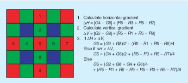
The Hamilton-Adams strategy [8] contains a key observa-tion describing the relaobserva-tions between the green channel and the other ones. In this algorithm the evaluation of the gradient at a missing green pixel is corrected by the second order derivatives of the red (blue) channel. More precisely, to estimate the green value at a pixel p= (i, j), where u(i, j) is known, u ∈ {b, r},

the method computes the following magnitudes, where v, h

mean “vertical”, “horizontal” (see Fig. 1):

Dh= |g(i, j−1)−g(i, j+1)|+|2u(i, j)−u(i, j−2)−u(i, j+2)|,

Dv= |g(i−1, j)−g(i+1, j)|+|2u(i, j)−u(i−2, j)−u(i+2, j)|. These magnitudes measure how flat the image is in the vertical and horizontal direction. If Dh< Dv the new green value is obtained by a horizontal interpolation

g(i, j) = (g(i − 1, j) + g(i + 1, j))/2

+(2u(i, j) − u(i − 2, j) − u(i + 2, j))/4.

If Dv< Dh, a vertical interpolation is applied,

g(i, j) = (g(i, j − 1) + g(i, j + 1))/2

+(2u(i, j) − u(i, j − 2) − u(i, j + 2))/4.

In the case that neither the horizontal nor vertical direction prevails, the new green value at pixel p= (i, j) is computed

as the average of the two previous values. Fig. 1 shows the geometric situation. The aim is to interpolate the green value at

Figure 1. Hamilton-Adams scheme for the interpolation of a green value at a red position.

pixel 5. First, a horizontal and a vertical oscillation measure are computed. This oscillation measure combines two color channels by adding the absolute value of the discrete green gradient to the absolute value of the red (or blue) discrete second derivative. This combination of estimates based on different colors is necessary. Indeed, at the red pixel 5 only red pixels are available for computing a horizontal or a vertical second derivative. But since the neighboring pixels are green, a vertical and a horizontal gradient can be computed with green pixels.

This method results in the green channel inheriting the high frequency (directional Laplacian) of the sub-sampled red or blue channels. Indeed, rewriting for example the horizontal interpolation, we get

g(i, j)−g(i + 1, j) + g(i − 1, j)

2 = −

u(i − 2, j) − 2u(i, j) + u(i + 2, j)

4 .

(1) Interpreting the above finite differences as differential opera-tors and using Theorem 1, this can be rewritten as

Chrominance regularity assumption

Letu = r or b. Then

|D(g − u)|curv(g − u) = 0.

In other terms,g − u has a zero second derivative in its least

variation direction.

Of course the least variation is only computed between the horizontal and vertical direction. Now, the underlying smooth-ness assumption has no reason to give a privilege to horizontal and vertical directions. As mentioned in the introduction, the Hirakawa et al. [9], Chung et al. [14], Menon et al. [10], and Zhang et al. [11] algorithms all involve the above step in that they try to select a least variation interpolation direction for the chromatic components.

IV. SELF-SIMILARITY DRIVEN COLOR SUPER-RESOLUTION

All above mentioned algorithms do not involve the recent progress in image structure implicit in the Efros-Leung algo-rithm. This algorithm takes advantage of image self-similarity to recreate textures from small samples. By comparing the im-age with itself, it recovers missing values by transporting them from places where they are known. The assumption underlying the proposed demosaicing algorithm is the following:

(5)

Figure 2. The pixel q3 in the hat has the same noisy grey level as

the reference pixel p. However, a comparison of the patches around p and q3shows that these pixels have different models, while the pixels

q1and q2obey the same model as p. Thus, patch comparison allows

one to infer the color model at a given pixel by using information contained far enough in the image. This key image property was first used by Efros and Leung [19] and opens the way to a self-similarity driven demosaicking.

Color information present in the raw image is redundant, and can be transported from pixels where it is known to pixels where it is missing based on local similarities.

A similar principle has already be briefly tested for demosaicking. Mairal et al. [22] proposed to adapt to demosaicking a denoising and inpainting algorithm based on a sparse representation obtained from a learned dictionary of image patches. They obtained excellent demosaicking results on some examples by this completely non-local strategy. The method is nonetheless rather a demonstration of the power of K-SVD classification and sparse representations, than a realistic demosaicking algorithm. Indeed, the dictionary must be learned for each image.

The Efros-Leung method cannot be applied to demosaicking without a strong revision. The first one is that a careful interpolation must proceed at the first steps with averages, as was proposed in the NL-means algorithm. Thus, we shall start with a short explanation of this denoising algorithm.

A. Non local denoising (NL-means algorithm)

The NL-means algorithm [20], [30] denoises a pixel x by averaging the values of all pixels whose Gaussian neighbor-hood looks like the neighborneighbor-hood of x.

N L[u](x) = 1 C(x) Z Ω e−h21 R R2Ga(t)|u(x+t)−u(y+t)| 2 dt u(y) dy, (2) where x ∈ Ω, C(x) = R_Ωe−h21 R R2Ga(t)|u(x+t)−u(y+t)| 2 dtdy is a normalizing constant, Ga is a Gaussian kernel and h acts as a filtering parameter. The parameter h controls the

decay of the exponential function and therefore the decay of the weights as a function of the Euclidean distances. NL-means is a generalized neighborhood filter. Neighborhood filters restore a pixel by taking an average of the values of neighboring pixels. These filters where invented and reinvented several times in image processing under various names: Lee [31] (sigma-filters), Yaroslavsky [32] (neighborhood filters),

Figure 3. The right-hand side of each pair shows the weight distribution used to estimate the central pixel of the left image by the NL-means algorithm. White pixels are similar to the central pixel of the left-hand image and have a high weight in the average.

Smith and Brady (SUSAN filter) [33], and more recently Tomasi and Manduchi [34] (bilateral filter). Neighborhood filters perform well in presence of moderate noise, but the comparison of the grey level or color values at a single pixel is no more robust when these values get noisier. This drawback is overcome by the non-local-means algorithm, that not only compares the grey level or color in a single point but the whole patch around them. This patch comparison permits a reliable similarity measure involving pixels which can fall far away from each other (see Fig. 2). This permits a non-local strategy and the systematic use of all possible self-predictions the image can provide, in the spirit of Efros and Leung [19]. The patch comparison also makes weight distributions in the mean computing the denoised value adapt to the local geometry of the image, as shown in Fig. 3. For a more exhaustive description of NL-means and neighborhood filters and a comparison with other denoising algorithms we refer to [20], [30].

B. Monochromatic self-similarity driven super-resolution

As pointed out in [27], super-resolution and demosaicking are two instances of a same problem: Both of them address the aliasing issue. Let u denote an aliased grey level image and

assume we want to duplicate its number of pixels by inserting a quincunx grid. This is exactly the situation we are in, since we wish to interpolate the green channel in the CFA mask. LetΩu denote the subset of the image grid where the values ofu are available. A first move, common to most algorithms,

is to interpolate the missing pixels by a classical algorithm, be it bi-linear, median or anisotropic interpolation. This yields a first estimate u0. This first rough approximation is blurry and can have erroneous structures and artifacts. In order to correct the interpolated values, a variant of the NL-means algorithm can be applied, that averages only pixels belonging

toΩu and transports this average only to pixels not belonging

to Ωu (unknown values). This conjunction of averaging and transportation is in essence what is proposed here. The window distances are computed on the initial estimateu0 (thus using

(6)

the interpolated values). The adaptation of formula (2) is N L[u](x) = 1 C(x) Z Ωu e−h21 R R2Ga(t)|u0(x+t)−u0(y+t)| 2 dt u(y) dy, (3) where x is the new-interpolated pixel (x ∈ Ω/ u) andC(x) is the normalization factor.

C. A self-similarity driven strategy

The essential difference with NL-means is that the final aim is not to denoise, but instead to infer high frequency

information by transportation from known pixels to unknown pixels. In the denoising case averaging pixels is a way to

reduce oscillations due to noise, and the value of the resolution parameter h depends on the noise standard deviation. In our

case instead, the value ofh should tend to zero, since we do

not want to reduce the oscillations but to transfer or copy the known values to pixels where they are unknown.

If the initial guess u0 has several artifacts or erroneous structures (which it is usually the case), then looking for similar pixels and copying their grey level values can lead to the reinforcement of these artifacts. For this reason, the algorithm is coarse to fine. It first reconstructs the large scale structures and iteratively refines the search by reducing the value ofh. This amounts to applying the formula (3) iteratively

with a decreasing sequence of values of h. When h is large

the interpolated values are blurry but reliable, and when h is

small the algorithm propagates values rather than averaging them.

Figure 4 displays the application of this algorithm to the in-terpolation of the missing green pixels of an image. We display this application for various sequences with decreasing values of h. This experiment shows that an iterative procedure is

necessary to reconstruct the erroneous interpolated structures of the initial condition. Only when the initial smoothing is strong enough, for h = 32 or 64, the global structure

domi-nates the erroneous local one. This reconstruction is compared to the one performed by classical algorithms which are often used to interpolate the green channel, namely the bi-linear interpolation, the median interpolation and the anisotropic interpolation.

D. Adaptation to the mosaicked image

The previous one-image self-similarity driven super-resolution method is easily adapted to the incomplete color image. Each channel is restored by averaging the original CFA values, the window distances being computed on the initial color image u0. The averaging process reads

N L[u](x) = 1 Cu(x) Z Ωu e−h21 R R2Ga(t)ku0(x+t)−u0(y+t)k 2 d_{t u(y) dy,} (4) withu ∈ {r, g, b}, x /∈ Ωu and Cu(x) = Z Ωu e−h21 R R2Ga(t)ku0(x+t)−u0(y+t)k 2 dtdy.

The missing values of each channel at a point x are interpo-lated by averaging original CFA values of the same channel

Figure 4. Gray interpolation experiment for various decreasing values of the parameter h. From left to right: initial image, bi-linear interpolation, median based interpolation, anisotropic interpo-lation and the result of the similarity driven demosaicking algorithm for the decreasing sequences of values for h, {4, 1}, {16, 4, 1}, {32, 16, 4, 1} and {64, 32, 16, 4, 1}. The initial condition is always

given by the median.

with a similar color Gaussian neighborhood in u0. In other terms, color inter-correlation is enforced by computing the distance in the three-channel image. As mentioned before, in order to gradually correct the erroneous structures and artifacts of u0 a coarse to fine strategy that refines at each step the similarity search by reducing the value ofh is crucial.

We should note that the similarity driven demosaicking algorithm might reduce some small oscillations caused by noise. This reduction is not drastic, since first a small value ofh ends the process, meaning that in the final iteration only

pixels having extremely similar windows around are averaged, and second denoising is not performed for known colors.

E. Implementation details

For computational purposes the search for similar pixels is restricted to a search window with size(2∗S +1)×(2∗S +1)

around each pixel. Even if many similar pixels can be found far away, there is usually enough information kept by taking a large search window. In all experiments a 15 × 15 pixels

search window was used.

The window comparison is performed by a flat Euclidean distance on a 3 × 3 neighborhood. This window has shown

to be robust (27 values) and small enough to take care of

details and fine structure. When dealing with grey image super-resolution or noisy images, the size of the window should increase to have a robust comparison. This is not considered in this paper, that deals with good quality color images.

The gaussian kernelGaintroduced in the general algorithm formulation (4) is only necessary as the size of the window increases. With the small3×3 window used here, the gaussian

weight is unnecessary. Thus, the implemented algorithm is just a simplest discrete version of formula (4). It computes a weighted sum of pixels in a15 × 15 neighborhood around the

reference pixel. The discrete formula is

N L[u](p) = 1 Cu(p) X q∈Ωu e− 1 h2 P t∈Wku0(p+t)−u0(q+t)k 2 u(q), (5)

(7)

withu ∈ {r, g, b}, p /∈ Ωu and Cu(p) = X q∈Ωu e−h21 P t∈Wku0(p+t)−u0(q+t)k 2 ,

where W is the 3 × 3 discrete window centered at (0, 0).

F. Implementing chromatic regularity

In contrast with all mentioned algorithms the similarity driven algorithm does not involve at this point any color regularization step. Indeed, it merely transports color values from known to unknown positions. In case of error, this involves a high risk of impulse noise. Typically, impulse noise can be corrected by a very local (3 × 3 median filter),

which will be added as a second step to SDD. Theorems 1 and 2 explain why this second step amounts to applying the Hamilton-Adams assumption on chrominance regularity. But, since the similarity driven super-resolution step fills in all color channels, the chromatic regularity assumption can be applied to the chrominance (U, V ) instead of the differences red − green and blue − green. Recall that

Y = ar r + ag g + ab b, U = r − Y, V = b − Y, withar= 0.299, ag= 0.587 and ab= 0.114. Notice that the green dominates in this linear combination. This coordinate system aims at separating the geometric information contained in Y from the chromatic information U, V , and gives more

importance to the green channel.

Chromatic regularity Step (CR)

1) Decompose the color image into the YUV components. 2) Perform a median of the coordinatesU and V in a 3 × 3 neighborhood obtaining U0 and V0. This median is applied to all the pixels independently of the CFA mask. 3) Recompose Y U0V0 into the RGB components.

4) Put back the original values of the CFA mask at pixels where they are known.

G. The proposed demosaicking algorithm

The final method alternates each iteration of the self-similarity driven algorithm with the chromatic regularity step

CR(u). This final strategy can be algorithmically described

by the following pseudo-code which takes as input the values of the CFA mask,I,

u0 <- Initial_Interpolation(I); for h in {16,4,1} do { u <- NL_h(u0); u <- CR(u); u0 <- u; } Output <- u; V. EXPERIMENTS

This section is devoted to a detailed performance compari-son. Experiments are performed on simulated mosaic images from the Kodak collection [35], which is widely used for that purpose (see Figure 5). As requested by several referees, we also incorporate experiments with the IMAX collection

1 _{recently introduced in [5] (see Figure 6). Images in both}

databases take integer color values between 0 and 255. Images in the Kodak collection have fewer color saturated regions, but are challenging by their Nyquist frequency details, that threaten strong aliasing. The IMAX database has many more saturated colors and edges separating colored regions. This strong difference is illustrated by the following statistics: The mean saturation of the Kodak database is15 while for the

IMAX database it is30. The mean value of the gradient of the

chromatic components is1.75 in the Kodak database while it

is6.21 in IMAX. At a first sight images in the IMAX database

seem more natural than images in the Kodak database. We compared the best algorithms according to the three reviews [4], [3], [5]: Hamilton-Adams, Hirakawa et al., Gun-turk et al., Li et al., Chung et al., Menon et al., Zhang et al., and Paliy et al. Each algorithm in the comparative experiments is used with its default parameters as given in the corresponding papers. We implemented all algorithms, except for the Hirakawa et al., Zhang et al. and Paliy et al. for which a Matlab code was downloaded from their respective web pages 2 3 4. For the proposed algorithm SDD the very same value of the parameters was also fixed once and for all: The color comparison window is3 × 3 pixels, the search window

zone is 15 × 15 pixels, and the decreasing sequence for h

is h = {16, 4, 1}. The Hamilton-Adams algorithm was used

as initial guess u0 for the SDD algorithm. Most compared algorithms actually also initialize with Hamilton-Adams, or equivalently start by selecting a direction interpolation that is an improvement of Hamilton-Adams. In other terms, all com-pared algorithms improve directly or indirectly on Hamilton-Adams. Thus, these respective improvements are the main object of the comparison. Probably the most striking feature is that this improvement is effective on the Kodak database but not at all on the IMAX database.

A brief summary of the results would be as follows. Zhang et al. and Paliy et al. are confirmed as the best algorithms in terms of mean square error for the Kodak basis. Paliy et al. is slightly better than Zhang et al. for the Kodak database. SDD and Menon et al. are slightly behind in terms of mean square error. From the visual viewpoint en Kodak, however, there is not much difference between Menon, SDD, Paliy, and Zhang. But, Paliy and SDD look slightly better, having a bit less zipper effect.

In Li et al. [5] review, Paliy et al. is pointed out as the best algorithm on Kodak but it is concluded that, in terms of mean

1_{We use 400 x 400 pieces of IMAX images which were kindly provided}

by X. Li

2_{Hirakawa et al. algorithm downloaded from http://www.csee.wvu.edu/ ˜}

xinl/source.html

3_{Zhang et al. algorithm downloaded from http://www4.comp.polyu.edu.hk/}

˜cslzhang/

4

(8)

Figure 5. Ten images of the Kodak collection [35]. Critical details extracted from these images will be used for comparative testing. They contain challenging details close to the Nyquist frequency.

Figure 6. Twelve images of the IMAX collection. They have much more color contrast than the Kodak database. Critical details extracted from these images will be used for comparative testing.

square error, none of the algorithms that attempted to improve the original Hamilton-Adams actually works satisfactorily on IMAX ! Even worse, the best mean square error would be as good as ever by interpolating independently each channel! We shall see that on the IMAX database, SDD and Hamilton-Adams are much better in MSE, but that, as far as zipper effect is concerned, Hamilton-Adams does not perform well.

Creation of color artifacts

Natural scenes contain large grey regions. False colors can be created in these zones by demosaicking algorithms. An excellent way to evaluate and quantify this artifact is to apply the algorithms to completely grey images. For that purpose, the images of Fig. 5 were converted into grey images. The best demosaicking result for the grey image would be obtained by simply setting r = g = b, one of these three values

being known at each pixel. Thus, every deviation from grey is actually an error. Algorithms creating colors from grey incur a high risk of creating wrong color spots. To evaluate this risk for all algorithms, the mean saturation of the demosaicked image was computed (Tables I and II). The saturation of a

(r, g, b) color is computed as its Euclidean distance in the 3D

Euclidean color space to the grey axis defined byr = g = b.

Tables I and II show that the methods creating less false colors are Zhang et al. [11] and Paliy et al. [5]. This means that very few color artifacts will be created by these methods in grey zones of the images. Since images in the Kodak database have very few color saturated region, these methods have a very good performance in this database. SDD, the POCS algorithm (Gunturk et al.) [16] and the demosaicking with directional filtering and a posteriori decision (Menon et al.)

[10] also perform well.

Zipper effect

Due to the configuration of the CFA mask, the green channel has one of every two pixel values fixed in each row and each column. When a demosaicking algorithm fails to interpolate the green channel, the interpolating artifacts only affect the unknown pixel values. Therefore, the interpolation artifacts are manifested as artificial ”on-off” image patterns. This effect was called ”zipper effect” in [18]. The zipper effect at a pixel is detected and numerically evaluated as an increase or a decrease of its contrast with respect to its most similar neighboring pixels, when passing from the original image to the demosaicked one. In other terms, zipper results in a coherent creation of local minima or maxima on a line or a grid. The percentage of pixels being affected by this artifact gives a zipper effect indicator for the tested algorithms. More precisely:

1) For each pixel p in the original image, identify the pixel

p∗ with minimum color distance within the set of eight neighboring pixels∆u0(p) = ku0(p) − u0(p∗)k. 2) Compute the color difference between the same pair of

pixels p and p∗ in the demosaicked imageu, ∆u(p).

3) Compute ϕ = ∆u0(p) − ∆u(p). A pixel p is affected by the zipper effect if |ϕ| > δ.

Tables III and IV give the zipper effect ratio of the compared methods for all images with detection thresholdδ = 2.5. The

zipper effect is commonly created when the red and blue channels have high frequencies that are different from the green ones (at such points the red or blue second derivatives are different from the green ones). For this reason, zipper effect concentrates on the edges separating colored regions.

Algorithms that impose the smoothness of the chromatic components (Zhang et al. and Paliy et al.) and the SDD exhibit a higher performance in the Kodak database. The POCS algorithm (Gunturk et al.) [16] shows a significantly higher zipper effect since it assumes that color responses are equal. The Homogeneity directed algorithm (Hirakawa et al.) [9] and the directional algorithm with a posteriori decision (Menon et al.) reduce the POCS zipper effect, since they choose between a horizontal and a vertical interpolation to reduce the number of created irregularities.

For the IMAX database all methods have a similar zipper effect except the SDD algorithm which exhibits a higher performance. Even the Hamilton-Adams algorithms exhibits a similar performance to Zhang et al. and Paliy et al. in this database. As we mentioned at the beginning of this section, the chromatic components of these images are not as smooth as those of the Kodak database.

Mean square error

The mean square error (MSE) is defined asP_i,j(u(i, j) − ˜

u(i, j))2_{, where} _{u is the reconstructed image and u the}_˜ original. Along with the peak signal-to-noise ratio it is the most common quality measurement. These measures are of course only computable on simulated mosaics, starting from a

(9)

Hamilton- Hirakawa Gunturk Li Chung Menon Zhang Paliy SDD -Adams et al. et al. et al. et al. et al. et al.

1 2.52 2.02 1.53 2.41 2.60 1.87 1.33 0.91 1.71 2 0.76 0.58 0.47 0.72 0.79 0.50 0.30 0.31 0.54 3 1.82 1.45 1.15 1.75 1.87 1.13 0.78 0.61 1.26 4 0.76 0.60 0.49 0.72 1.08 0.58 0.34 0.34 0.61 5 2.61 2.06 1.64 2.51 2.73 1.99 1.45 1.04 1.61 6 1.01 0.82 0.63 0.96 1.06 0.75 0.53 0.51 0.74 7 1.09 0.88 0.67 1.04 1.18 0.82 0.55 0.51 0.86 8 1.46 1.16 0.90 1.39 1.49 1.09 0.76 0.67 1.05 9 1.49 1.21 0.92 1.42 1.44 1.11 0.75 0.64 1.13 10 0.71 0.57 0.45 0.67 0.75 0.53 0.33 0.34 0.57 Avg 1.42 1.14 0.89 1.36 1.5 1.04 0.71 0.59 1.01 Table I

EVALUATION OF THE CREATION OF FALSE COLORS. DEMOSAICKING METHODS ARE APPLIED TO THE GREY LEVEL VERSION OF IMAGES IN THEKODAK DATABASE AND THE MEAN SATURATION OF DEMOSAICKED IMAGES IS DISPLAYED(SEE THE TEXT FOR MORE DETAILS).

1 1.66 1.35 1.03 1.59 1.85 1.26 0.82 0.67 1.18 2 2.26 1.78 1.32 2.15 2.63 1.60 0.93 0.57 1.61 3 0.98 0.76 0.61 0.93 1.32 0.76 0.41 0.28 0.87 4 1.48 1.16 0.89 1.41 1.88 1.09 0.62 0.38 1.20 5 0.62 0.49 0.41 0.59 0.91 0.48 0.22 0.17 0.67 6 1.13 0.92 0.70 1.07 1.51 0.86 0.45 0.30 0.91 7 0.73 0.59 0.48 0.70 1.11 0.57 0.29 0.25 0.72 8 0.56 0.46 0.38 0.53 0.73 0.43 0.23 0.24 0.53 9 0.63 0.51 0.42 0.60 0.72 0.50 0.31 0.32 0.56 10 0.77 0.62 0.51 0.73 0.80 0.61 0.39 0.37 0.68 11 1.10 0.86 0.67 1.04 1.28 0.81 0.42 0.39 0.93 12 1.11 0.92 0.70 1.07 1.19 0.83 0.54 0.50 0.91 Avg. 1.09 0.87 0.68 1.03 1.33 0.82 0.47 0.37 0.9 Table II

EVALUATION OF THE CREATION OF FALSE COLORS. DEMOSAICKING METHODS ARE APPLIED TO THE GREY LEVEL VERSION OF IMAGES IN THEIMAX

DATABASE AND THE MEAN SATURATION OF DEMOSAICKED IMAGES IS DISPLAYED(SEE THE TEXT FOR MORE DETAILS).

1 2.90 2.61 2.38 2.70 3.26 2.21 1.70 1.28 2.03 2 1.15 1.29 1.06 1.02 1.30 0.85 0.58 0.46 0.51 3 1.96 1.88 1.54 1.75 2.37 1.26 0.91 0.84 1.38 4 0.83 1.21 1.39 0.76 2.13 0.83 0.62 0.45 0.41 5 2.91 2.42 2.79 2.79 3.29 2.52 1.91 1.59 1.84 6 1.78 2.74 1.41 1.36 1.98 1.44 0.82 0.84 0.71 7 1.61 2.13 0.87 1.22 1.83 1.15 0.69 0.70 1.00 8 1.79 2.08 1.34 1.54 1.94 1.44 0.95 0.94 1.05 9 1.41 1.75 1.41 1.30 1.69 1.36 1.00 1.04 1.04 10 1.00 1.58 1.06 0.85 1.15 1.03 0.57 0.57 0.52 Avg 1.73 1.96 1.53 1.53 2.09 1.41 0.98 0.87 1.05 Table III

ZIPPEREFFECT INRGBCOORDINATES FOR THEKODAK COLLECTION(δ=2.5).

1 0.26 0.17 0.55 0.41 0.36 0.34 0.23 0.19 0.11 2 0.09 0.07 0.12 0.12 0.11 0.10 0.10 0.12 0.05 3 0.30 0.31 0.57 0.38 0.41 0.40 0.35 0.37 0.18 4 0.19 0.18 0.30 0.23 0.25 0.22 0.19 0.25 0.12 5 0.32 0.33 0.65 0.40 0.40 0.43 0.40 0.36 0.17 6 0.15 0.16 0.26 0.18 0.18 0.19 0.17 0.19 0.07 7 0.14 0.16 0.24 0.16 0.17 0.18 0.15 0.14 0.06 8 0.12 0.16 0.27 0.14 0.17 0.20 0.16 0.15 0.06 9 0.13 0.18 0.27 0.16 0.18 0.20 0.16 0.14 0.07 10 0.10 0.14 0.13 0.11 0.14 0.13 0.10 0.11 0.06 11 0.10 0.17 0.14 0.10 0.12 0.13 0.09 0.11 0.02 12 0.09 0.10 0.18 0.12 0.12 0.12 0.11 0.11 0.07 Avg 0.17 0.17 0.31 0.21 0.22 0.22 0.18 0.19 0.09 Table IV

(10)

known original image. MSE does not necessarily reflects the visual quality of the output image [19], [36]. It remains all the same an inescapable quality criterion. Note that the range of the pixel values in our tests is [0255].

Table V shows that Zhang et al. and Paliy et al. perform slightly better in terms of MSE than Gunturk et al, Menon et al. and SDD. As we mentioned the Zhang et al. and Paliy et al. algorithms are also the ones creating less false colors when applied to grey zones of images. Despite its good performance in MSE, the Gunturk et al. and Menon et al. algorithms introduce more zipper effect.

However, for the IMAX database (table VI) the Hamilton-Adams and SDD give the best MSE. Indeed, the strong zipper effects of Zhang et al. and Paliy et al. increase the MSE. This zipper effect is mainly concentrated near edges, and therefore a serious perceptual interference. The SDD MSE is coherent with a low zipper effect.

Computation time

The computational cost of SDD lies in the computation of patch distances. For each pixel the distance of a 3 × 3

color patch with patches contained in a 15 × 15 neighborhood

must be computed. There is fortunately a restriction, that the color channel in each compared pixel must be different from the one known at the current pixel. The total cost is

27 ×5₈× 225 ≃ 2109 operations per pixel. This puts SDD at

a computational cost higher than basic directional filters, and comparable to more sophisticated algorithms. Multi-resolution and preselection strategies can actually be used to further accelerate these patch comparisons, as proposed in [20], [37].

Visual quality

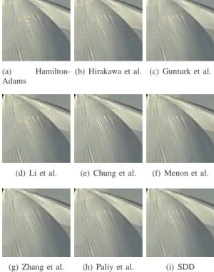
In general, a low performance in one of the previous three numerical criteria also entails a rejection by a human visual inspection. In spite of this, none of these criteria can fully replace human evaluation, because of the very diverse geometric situations in images, and of the varying visual impact of each error, depending on the context. For this reason, a human visual evaluation still is the most important criterion to judge the performance of demosaicking algorithms. This performance must be evaluated on edges, textures, and various kinds of geometric details such as corners, diagonals, and fine patterns. Figures 7, 8, 9 and 10 furnish a wide-ranging comparative visual quality assessment of demosaicked images. Figure 7 illustrates how the recently developed directional filters and the homogeneity directed algorithm (Hirakawa et al.) [9] are able to restore a grey and nearly vertical high frequency pattern. This figure also illustrates how the POCS algorithm (Gunturk et al.) [16] outperforms the successive approximation algorithm (Li) [15].

Figure 8 points out how all algorithms fail near the corners, or when patterns with several orientations meet, even though the image region is mainly grey. Only Paliy et al. and SDD give a fully visually acceptable solution in that case. Figure 9 illustrates the strong residual zipper effect left by the POCS algorithm (Gunturk et al.) and all directional filters. The first

(a) Hamilton-Adams

(b) Hirakawa et al. (c) Gunturk et al.

(d) Li et al. (e) Chung et al. (f) Menon et al.

(g) Zhang et al. (h) Paliy et al. (i) SDD

Figure 7. Aliasing and color. The first four algorithms present many color aliasing and spots since they are not able to correctly choose between a horizontal or vertical interpolation. The four last algorithms reconstruct accurately the original. This figure shows that the recent directional filters improve the original homogeneity directed algorithm of Hirakawa et al. SDD yields a result comparable to the best directional filters and Zhang et al. and Paliy et al.

one fails because of an excessive color frequency copy from one channel to the others, while the directional filters seem to fail because of the inability to interpolate diagonal patterns.

Finally, figure 10 shows the strong zipper effect of most methods in the IMAX database, where edge colors predom-inate. Such edge colors are rare in the Kodak database. Somehow, the Kodak database focuses on the reconstruction of luminance high frequencies in grey regions, while the IMAX database challenges the ability of algorithm to keep up with color edges. Only SDD and Hamilton-Adams are able to give a reasonable solution.

VI. CONCLUSION

The new-proposed demosaicking algorithm takes advantage of self-similarities in natural images to interpolate by trans-porting known values to missing values. Many experiments on two different databases have shown that it is possible to restore thin and fine periodic structures without creating zipper effects in others. An important feature of the new-introduced method is that it can extend immediately to movies. In the case of a movie, the search window can be extended to involve several successive frames, thus providing more patches, and a much more obvious self-similarity. Further work will focus on acceleration issues to apply the same ideas to real-time video processing. The complementary comparative experiments asked by several of our seven referees have shown a disturbing disparity in algorithm performance depending on

(11)

Hamilton- Hirakawa Gunturk Li Chung Menon Zhang Paliy SDD

-Adams et al. et al. et al. et al. et al. et al.

1 26.91 20.06 10.60 22.20 27.57 14.12 9.16 5.85 15.52 2 6.18 5.06 5.37 5.68 7.01 4.36 3.48 2.94 4.27 3 20.73 11.43 8.98 17.29 18.82 8.27 6.14 5.25 11.64 4 5.41 5.85 4.53 4.87 9.75 4.29 3.78 3.27 4.72 5 40.36 27.54 18.57 33.97 38.51 21.94 16.20 12.68 21.36 6 6.09 5.17 4.52 5.33 7.41 3.87 3.18 2.93 4.78 7 9.41 7.83 5.24 7.98 10.45 6.02 4.35 4.34 7.01 8 12.01 9.73 6.69 10.22 13.55 7.04 5.14 4.62 8.41 9 15.86 15.37 12.47 14.26 17.08 12.16 9.33 9.26 13.76 10 4.43 4.55 4.55 4.12 6.41 3.71 3.08 2.68 4.35 Avg 14.74 11.2 8.15 12.59 15.66 8.58 6.38 5.38 9.58 Table V

MEAN SQUARE ERRORS INRGBCOORDINATES FOR THEKODAK COLLECTION.

Hamilton- Hirakawa Gunturk Li Chung Menon Zhang Paliy SDD

-Adams et al. et al. et al. et al. et al. et al.

1 98.22 133.41 168.22 139.10 114.90 110.10 105.92 101.56 100.12 2 92.18 120.15 143.72 122.45 114.97 105.55 101.52 145.03 100.47 3 43.52 63.94 80.79 49.43 54.19 53.38 47.65 49.22 42.31 4 47.27 63.62 79.40 50.83 59.50 55.03 48.55 64.22 49.44 5 33.43 59.51 74.19 39.44 43.60 49.15 46.02 36.85 33.15 6 40.07 60.17 76.64 44.37 53.87 51.91 47.01 52.09 40.79 7 21.99 31.73 43.67 24.60 30.92 27.79 25.99 23.32 21.54 8 11.60 14.81 21.30 12.83 14.74 13.50 12.80 10.51 9.55 9 8.33 9.83 11.67 8.72 10.52 9.42 8.43 7.86 6.85 10 8.09 10.04 10.22 8.31 9.83 9.04 8.28 8.25 7.85 11 28.73 42.81 44.98 30.34 36.07 33.57 32.74 33.80 30.54 12 25.08 28.23 37.56 25.73 28.64 25.39 24.77 24.09 23.61 Avg 38.21 53.18 66.03 46.35 47.65 45.32 42.47 46.4 38.85 Table VI

MEAN SQUARE ERRORS INRGBCOORDINATES FORIMAXCOLLECTION.

the choice of the benchmark database. It seems that most algorithms have been designed to keep up with the presence of Nyquist frequencies in grey image regions of the Kodak database. Unfortunately these sharp algorithms have a much poorer behavior in presence of the color edges of the IMAX database. Thus, it seems that the creation of a database that would retain all disturbing features and respect actual image statistics is strongly needed.

REFERENCES

[1] B. Bayer, “Color imaging array,” 1976, uS Patent 3,971,065. [2] D. Alleysson, S. Susstrunk, and J. Herault, “Linear Demosaicing

In-spired by the Human Visual System,” Image Processing, IEEE

Trans-actions on, vol. 14, no. 4, pp. 439–449, 2005.

[3] D. Alleyson, “1-30 ans de d´emosa¨ıc¸age,” Traitement du Signal, vol. 21, no. 6, pp. 561–581, 2004.

[4] B. Gunturk, J. Glotzbach, Y. Altunbasak, R. Schafer, and R. Mersereau, “Demosaicking: color filter array interpolation,” Signal Processing

Mag-azine, IEEE, vol. 22, no. 1, pp. 44–54, 2005.

[5] X. Li, B. Gunturk, and L. Zhang, “Image demosaicing: a systematic survey,” Proceedings of SPIE, vol. 6822, p. 68221J, 2008.

[6] D. Cok, “Signal processing method and apparatus for producing inter-polated chrominance values in a sampled color image signal,” 1987, uS Patent 4,642,678.

[7] R. Hibbard, “Apparatus and method for adaptively interpolating a full color image utilizing luminance gradients,” 1995, uS Patent 5,382,976. [8] J. Hamilton Jr and J. Adams Jr, “Adaptive color plan interpolation in

single sensor color electronic camera,” 1997, uS Patent 5,629,734. [9] K. Hirakawa and T. Parks, “Adaptive homogeneity-directed demosaicing

algorithm,” Image Processing, IEEE Transactions on, vol. 14, no. 3, pp. 360–369, 2005.

[10] D. Menon, S. Andriani, and G. Calvagno, “Demosaicing With Direc-tional Filtering and a posteriori Decision,” Image Processing, IEEE

Transactions on, vol. 16, no. 1, pp. 132–141, 2007.

[11] L. Zhang and X. Wu, “Color demosaicking via directional linear mini-mum mean square-error estimation,” Image Processing, IEEE

Transac-tions on, vol. 14, no. 12, pp. 2167–2178, 2005.

[12] D. Paliy, V. Katkovnik, R. Bilcu, S. Alenius, and K. Egiazarian, “Spatially adaptive color filter array interpolation for noiseless and noisy data,” INTERNATIONAL JOURNAL OF IMAGING SYSTEMS

AND TECHNOLOGY, vol. 17, no. 3, p. 105, 2007.

[13] V. Katkovnik, K. Egiazarian, and J. Astola, “Adaptive Window Size Image De-noising Based on Intersection of Confidence Intervals (ICI) Rule,” Journal of Mathematical Imaging and Vision, vol. 16, no. 3, pp. 223–235, 2002.

[14] K. Chung and Y. Chan, “Color demosaicing using variance of color differences.” IEEE Trans Image Process, vol. 2006, pp. 2944–55, 1910. [15] X. Li, “Demosaicing by successive approximation,” Image Processing,

IEEE Transactions on, vol. 14, no. 3, pp. 370–379, 2005.

[16] B. Gunturk, Y. Altunbasak, and R. Mersereau, “Color plane interpolation using alternating projections,” Image Processing, IEEE Transactions on, vol. 11, no. 9, pp. 997–1013, 2002.

[17] N. Lian, L. Chang, Y. Tan, and V. Zagorodnov, “Adaptive Filtering for Color Filter Array Demosaicking,” Image Processing, IEEE

Transac-tions on, vol. 16, no. 10, pp. 2515–2525, 2007.

[18] W. Lu and Y. Tan, “Color filter array demosaicking: new method and performance measures,” Image Processing, IEEE Transactions on, vol. 12, no. 10, pp. 1194–1210, 2003.

[19] A. Efros and T. Leung, “Texture synthesis by non-parametric sampling,”

International Conference on Computer Vision, vol. 2, no. 9, pp. 1033–

1038, 1999.

[20] A. Buades, B. Coll, and J. M. Morel, “A review of image denoising algorithms, with a new one,” Multiscale Modeling Simulation, vol. 4, no. 2, pp. 490–530, 2005.

[21] A. Buades, B. Coll, and J. Morel, “A non-local algorithm for image denoising,” IEEE Computer Society Conference on Computer Vision and

Pattern Recognition, vol. 2, pp. 60–65, 2005.

[22] J. Mairal, M. Elad, and G. Sapiro, “Sparse Representation for Color Image Restoration,” Image Processing, IEEE Transactions on, vol. 17, no. 1, pp. 53–69, 2008.

(12)

(a) Hamilton-Adams

Figure 8. Wrong directions. This figure shows how difficult it is for all algorithms to make guesses at corners or at crossing points. Only Paliy et al. and SDD give a fully visually acceptable solution.

[23] K. Hirakawa and T. Parks, “Joint demosaicing and denoising,” IEEE

Trans. Image Processing, vol. 15, no. 8, pp. 2146–2157, 2006.

[24] R. Ramanath and W. Snyder, “Adaptive demosaicking,” Journal of

Electronic Imaging, vol. 12, p. 633, 2003.

[25] L. Zhang, X. Wu, and D. Zhang, “Color Reproduction From Noisy CFA Data of Single Sensor Digital Cameras,” Image Processing, IEEE

Transactions on, vol. 16, no. 9, pp. 2184–2197, 2007.

[26] X. Wu and L. Zhang, “Temporal color video demosaicking via motion estimation and data fusion,” IEEE Transactions on Circuits and Systems

for Video Technology, vol. 16, no. 2, pp. 231–240, 2006.

[27] S. Farsiu, M. Elad, and P. Milanfar, “Multiframe demosaicing and super-resolution of color images,” IEEE Transactions on Image Processing, vol. 15, no. 1, pp. 141–159, 2006.

[28] X. Wu and L. Zhang, “Improvement of color video demosaicking in temporal domain.” IEEE Trans. Image Processing, vol. 15, no. 10, pp. 3138–3151, 2006.

[29] F. Guichard and J. Morel, “Introduction to Partial Differential Equations in Image Processing.” 1995.

[30] A. Buades, B. Coll, and J. Morel, “Image and movie denoising by non-local means,” Int. Journal of Computer Vision, to appear in 2007. [31] J. Lee, “Digital image smoothing and the sigma filter,” Computer Vision,

Graphics, and Image Processing, vol. 24, pp. 255–269, 1983.

[32] L. Yaroslavsky, Digital Picture Processing. Springer-Verlag New York, Inc. Secaucus, NJ, USA, 1985.

[33] S. Smith and J. Brady, “SUSAN-A New Approach to Low Level Image Processing,” International Journal of Computer Vision, vol. 23, no. 1, pp. 45–78, 1997.

[34] C. Tomasi and R. Manduchi, “Bilateral filtering for gray and color images,” Proceedings of the Sixth International Conference on Computer

Vision, p. 839, 1998.

[35] “Kodak true color image collection,” http://r0k.us/graphics/kodak/. [36] P. Longere, X. Zhang, P. Delahunt, and D. Brainard, “Perceptual

assessment of demosaicing algorithm performance,” Proceedings of the

IEEE, vol. 90, no. 1, pp. 123–132, 2002.

[37] M. Mahmoudi and G. Sapiro, “Fast image and video denoising via nonlocal means of similar neighborhoods,” Signal Processing Letters,

IEEE, vol. 12, no. 12, pp. 839–842, 2005.

(a) Hamilton-Adams

Figure 9. Zipper on vertical edges. This figure illustrates the zipper effect provoked by the POCS algorithm (Gunturk et al.) and by all directional filters. The first one occurs because of erroneous color frequency copying, while the other ones fail because they are not fit to correctly interpolate diagonal patterns.

(a) Hamilton-Adams

Figure 10. Zipper effect on IMAX images. Most methods present a strong zipper effect on color edges that makes the demosaicked image not a reasonable solution to the demosaicking problem. Only the SDD algorithm and Hamilton-Adams are able to give a reasonable solution.