Exact out-of-equilibrium central spin dynamics from integrability

This content has been downloaded from IOPscience. Please scroll down to see the full text.

Download details:

IP Address: 134.21.47.136

This content was downloaded on 03/09/2014 at 11:19

Please note that terms and conditions apply.

Exact out-of-equilibrium central spin dynamics from integrability

View the table of contents for this issue, or go to the journal homepage for more 2014 New J. Phys. 16 043024

integrability

Davide Fioretto1,2, Jean-Sébastien Caux2and Vladimir Gritsev1,2 1_{Department of Physics, University of Fribourg, Chemin du Musée 3, 1700 Fribourg,}

Switzerland

2

Institute for Theoretical Physics, Universiteit van Amsterdam, Science Park 904, Postbus 94485, 1098 XH Amsterdam, The Netherlands

Received 21 January 2014, revised 24 February 2014 Accepted for publication 3 March 2014

Published 23 April 2014

New Journal of Physics 16 (2014) 043024

doi:10.1088/1367-2630/16/4/043024

Abstract

We consider a Gaudin magnet (central spin model) with a time-dependent exchange couplings. We explicitly show that the Schrödinger equation is ana-lytically solvable in terms of generalized hypergeometric functions for particular choices of the time dependence of the coupling constants. Our method estab-lishes a new link between this system and the SU 2 Wess

( )

–Zumino–Witten

model, and sheds new light on the implications of integrability in out-of-equi-librium quantum physics. As an application, a driven four-spin system is studied in detail.

Keywords: non-equilibrium physics, Gaudin magnets, Knizhnik–Zamolodchikov equations, quantum integrability

1. Introduction

The problem of describing the coherent out-of-equilibrium evolution of driven many-body quantum systems has attracted a great deal of attention in recent years. This interest was spurred by the recent advances in cold atoms and semiconductor physics, which made experimental observations possible. The attention of the community has mostly been devoted to the investigation of two limiting cases: the quench regime [1], where the variation of the parameters of the Hamiltonian is very fast with respect to all the other time scales of the problem, and the

Content from this work may be used under the terms of theCreative Commons Attribution 3.0 licence. Any further distribution of this work must maintain attribution to the author(s) and the title of the work, journal citation and DOI.

adiabatic regime, where it is slow (see [2] for a recent overview). Outside of these two extreme situations, very little is known, either analytically or numerically. This is unfortunate, because this driven regime has the most potential for novel physics.

There are natural obstacles for direct studies of non equilibrium quantum many-body systems: only a few solutions of the single-particle Schrödinger equation with time-dependent parameters are known even in the single-particle case. The situation is even worse in the many-body case. While integrable many-many-body systems provide considerable insight into equilibrium physics in one dimension, their non equilibrium behavior is still difficult to analyze because of the complexity of their solution. Numerical treatments of time-dependent systems (like e.g. by the time-dependent density-matrix renormalization group) are limited by the quantum entanglement which grows while the system evolves in time starting from some initial state [3–6]. To our knowledge there is a only a single subclass of systems where the full time dependence of parameters can be kept to some extent and where the dynamics can be understood in its full complexity. The dynamics of these systems can be mapped to the dynamics of a different systems which have no explicit time-dependence of parameters by an appropriate transformation of the coordinates, time, and wave-functions [7–12]. While this class of models is limited, it provides a clue about certain interesting and fundamental dynamical effects, like e.g. dynamical fermionization, and moreover it does not rely on integrability of the time-independent model.

To go beyond this class of models some new ideas are needed. Here we make an effort in this direction by suggesting to use a fact that the wave functions of a broad class of many-body quantum-mechanical models can be represented in terms of the correlation functions of some field theories with known properties. These connections were discovered and used in the context of the quantum Hall effect, where the quantum wave functions can be related to conformal blocks of the two-dimensional conformal field theories (CFTs) [13]. Interestingly, the wave functions of some integrable spin models can also be related to the correlators of certain CFTʼs [14, 15]. Here we extend and use these observations further to study non equilibrium dynamics of those spin models. Since these spin models belong to a broader class of a so-called Gaudin systems, our observations can be applied to that class as well. The central ingredient of our approach here is the fact that the conformal blocks of the 2D

Wess–Zumino–Witten (WZW) model are solutions of the Knizhnik–Zamolodchikov (KZ)

equation. For a broader class of CFTʼs (without internal symmetry) these equations should be replaced by the Belavin–Polyakov–Zamolodchikov system. We believe that the approach we explore here can be generalized further for systems with a more general matrix-product like structure of the wave functions.

Implementing the above ideas concretely, we investigate a model of N spin−1/2 degrees of freedom coupled by time-dependent exchange parameters J t_i( ),

∑

= · = − H_CS( )t J t S( ) S. (1) i N i i 1 1 0

Label 0 refers to the ‘central spin’ which is coupled to theN − 1 other (mutually uncoupled) spins. For time-independent couplings, this model is known as the central spin model, a Gaudin magnet [16–18]. Crucially, this Hamiltonian is directly relevant to experiments in quantum dots [19, 20] and nitrogen vacancy centers in diamond [21], in which time-dependent couplings are intrinsic to the experimental protocols (respectively via time-dependent gate voltages and

external electromagneticfields). The model (1) is only one of the broad class of models where dynamics can be treated using our method here. Other Gaudin-type models can be directly studied in a similar way.

The aim of this article is therefore twofold. On the one hand, we identify a time-dependent protocol for which it is possible to obtain analytical information (i.e. the exact many-body wavefunction) for a class of Hamiltonians related to the (1). While the requirements of this protocol are restrictive, they nonetheless allow to go beyond the adiabatic or sudden approximation. On the other hand, our technique points to an intriguing link between the time-dependent central spin Hamiltonian and the WZW model, a well-known CFT, opening the door to further applications of CFT techniques to driven nonequilibrium physics.

We note that here we will restrict our interests to the dynamics of the total spin-singlet subspace,S2 = 0. This is a good starting point because (see [22,23] and the recent review [24]) this subspace plays a crucial role in quantum information theory: the decoherence-free dynamics naturally occurs in this subspace, while the qubits can be encoded into its basis states.

2. Main results

We begin from the fact that the conformal blocks of the WZW model [25] satisfy the KZ equations [26]. For a SU 2

( )

k WZW model, these equations read

⎡ ⎣ ⎢ ⎢ ⎤ ⎦ ⎥ ⎥

∑

Ψ ∂ ∂ − · − … = ≠ − k z z z z z S S ( , , ) 0, (2) i j i i j i j N 0 N 1

where Ψ_N( ,z₀ …, z_N−1) = φ( )z₀ …φ(z_N−1) is the N-point holomorphic conformal block of primary field φ, while k is a number known as the level of the Kac–Moody algebra. If k is a positive integer, the WZW model is a rational CFT. Interestingly, there exist integral representations of solutions to the KZ equations that can be analytically continued to any nonzero complex k [27, 28].

Choosingk = iv wherev ∈  and considering the ansatz ψ ( )t = Ψ

(

z ( ),t …, z ₋ ( )t

)

N N 0 N 1

for a many-body wavefunction, we see that ψ ( )t

N can in fact be reinterpreted as a

time-dependent Schrödinger equationiψ˙ ( )t = H t( )ψ ( )t

N N with Hamiltonian 

∑∑

= ˙ · − = − ≠ H t z t v z t z t S S ( ) ( ) ( ) ( ). (3) i N j i i i j i j 0 1

Therefore, if z₀( )t is chosen to be the sole time-dependent parameter,

ψ_N( )t = Ψ_N

(

z₀( ),t z₁, …, z_N−1

)

solves the time-dependent Schrödinger equation for Hamilto-nian (1) with couplings

 = ˙ − J t z t v z t z ( ) ( ) ( ( ) ). (4) i i 0 0

It is shown in appendix A that this choice of time-dependent parameters z t_j( ) ( =j 0,…, N − 1) is uniquely dictated by the form of (1). Notice that the hermiticity of the Hamiltonian forces all thez_i to be on the same line in the complex plane (for example, we can take them to be all real).

Let us emphasize the main features of our approach. First of all, the main ingredient for an explicit solution of the time-dependent Schrödinger equation is a solution of the KZ equations that can be analytically continued to imaginary k. For small systems, this can be done explicitly, using standard CFT techniques. For larger systems, we can rely on a class of integral representations. Quite interestingly, these representations rely crucially on the integrability of the time-independent Hamiltonian, i.e. the off-shell Bethe equations. Therefore, the solubility of the time-dependent Schrödinger equation seems to be a signature of the underlying integrability of the model that survives also when the couplings are time dependent. Indeed, this interpretation is confirmed by the fact that, as we will discuss later on, the solvability of the time-dependent Schrödinger equation is not a special feature of the central spin model: our arguments apply also to the broader class of XXZ Gaudin magnets. Moreover, our results establish a new connection between theSU 2 WZW model (admittedly, for the quite unusual

( )

imaginary k case) and the time-dependent central spin Hamiltonian. It is worth to note here that theSU 2 WZW model is known to be related to integrable [

( )

14] and nonintegrable [29, 30] time-independent spin Hamiltonians. Finally, it is important to stress that—by construction— this approach works only if the time dependence of the J t_i( )isfinely tuned: essentially, the time evolution is ‘geometric’, i.e.

∫

dtH t( ) can be written as a curvilinear integral in the space of thez_j.

Our paper is organized as follows. First of all, in section3we provide a detailed analysis of a simple system of four spins. Thanks to the connection between the central spin Hamiltonian and the WZW model, we are able to analyze the time of evolution of the subspace of zero total spin in terms of hypergeometric functions. In this way, we can see our approach explicitly in action and understand some mathematical property of our solution (i.e. completeness and nontriviality). Therefore, in section 4, we move to a more general setting: a N particle XXZ Gaudin magnet with time-dependent couplings (4). Here, we take advantage of an integral representation of the solution of the (generalized) KZ equations to provide an integral representation for the time-dependent many-body wavefunction. While this representation is not (yet) amenable to an quantitative evaluation, it allows us to consider two interesting situations: the adiabatic and the semiclassical limit, thus gaining insight on the completeness of our solutions (section 4.1) . Finally, we present our conclusions in section 5, while some of the more technical details are discussed in the appendices.

3. A simple example: a four spins system

The class of Hamiltonians under consideration has a quite specific time-dependent coupling constant (4). Moreover, as we will see, in the general case, while it is possible to write down an integral representation for the wavefunction, it is not easy to extract physical predictions from it. The reader could wonder if this class of Hamiltonians can be solved only because their physics is trivial or if, instead, we can expect some interesting phenomenology that might motivate a further investigation of these systems. In this section, we want to address this point by studying one quite simple representative of this class of Hamiltonians: a central spin Hamiltonian with four constituents,

∑

= ˙ − · = H t v z t z t z S S ( ) 1 ( ) ( ) . (5) i i i 1 3 0 0 0

Since the total spin is conserved by the time evolution, we can restrict ourselves to the subspace with constantS2 = ∑

(

_iS_i

)

2. In the following, we would like to show that, indeed, the WZW correlators provide solutions that describe the whole zero spin subspace.

The computation of the four point conformal blocks Ψ z₄( ,₀ z z₁, ₂, z₃)of the WZW model is a standard exercise of CFT (see [25]). The detailed calculation is reported in appendixB, where

Ψ z₄( ,₀ z z₁, ₂, z₃) is expressed in terms of the standard hypergeometric functions _{2 1}F a b c x

(

, , ,

)

[31]. We introduce the parametrization Ψ₄( ,z₀ z z₁, ₂, z₃) =

[

(z₀ − z₃) (z₁ − z₂)

]

− kf x( )

3 4

, where

f x( ) is a function of the anharmonic ratio x = (₍z_z0₋−_zz1) (_{) (}z_z2−₋z_z3)₎

0 3 2 1 and expand ⎡⎣ ⎤⎦ =

(

−

)

− ∑₌ f x( ) x 1 x k _i2 ₁G x_i( ) v_i 3 4

on a basis of theS2 = 0subspace given by the two states

⎛ ⎝ ⎜ ⎞ ⎠ ⎟ ⎛ ⎝ ⎜ ⎞ ⎠ ⎟ ⎡ ⎣ ⎢ ⎛_⎝⎜ ⎞_⎠⎟ ⎛_⎝⎜ ⎞_⎠⎟⎤ ⎦ ⎥ = | + − 〉 − | − + 〉 ⊗ | + − 〉 − | − + 〉 = |++ − − 〉 + | − − ++〉 + | + − 〉 + | − + 〉 ⊗ | + − 〉 + | − + 〉 v v 2 2 , 1 3 2 2 . (6) 1 2

We thus can writeG x₁( ) = ∑_i2₌₁cw x_{i i}( ), where c_1,2 are constants determined by the initial conditions, while ⎜ ⎟ ⎜ ⎟ ⎛ ⎝ ⎞⎠ ⎛ ⎝ ⎞ ⎠ = − − − = − − + + + w x F k k k x w x x F k k k x ( ) 3 2 , 1 2 , 1 , , ( ) ( ) 1 1 2 , 1 2 2 1 , , (7) i k k 1 2 1 2 1 1 and G x( ) = −x

[

3G x( ) + 4k x G′ ( )x

]

x 2 1

3 1 1 . Therefore, as discussed above, the wavefunction

ψ ( )t = Ψ

(

z ( ),t z z, , z

)

4 4 0 1 2 3 (with k = iv) is a solution of the time-dependent Schrödinger

equation for Hamiltonian (5).

As an example, let us consider the following protocol. At time t = 0, the spins S_j, =

j 1, 2, 3, are at a distance j from the central spin S₀. Their couplings J_j are taken to be proportional to j−3 (dipolar interaction) or to exp

(

−j2

)

(shell model). Subsequently for >t 0, the coupling constants decrease inverse linearly in time (plus a site-dependent term). We can thus model this situation withz₀ = ωtandz_j = −j3(dipolar interaction) orz_j = −exp

( )

j2 (shell model), j= 1, 2, 3.

The first thing to analyze is the completeness of the solution, i.e. if the space spanned by the conformal blocks solution is bidimensional. It is shown in appendix B that the absolute value of the determinant of the matrix M_ij

(

x t( )

)

such that G x t_i

(

( )

)

= ∑_jM_ij

(

x t( )

)

c_j is actually constant and nonvanishing fort ∈

[

0, +∞

)

, thus proving that this family of solutions

spans the whole subspace of zero total spin. This fact is unrelated to our choice of z₀( )t andz_i

and remains true for any parametrization (see appendix B).

As an application, an interesting quantity to look at is the modulus square of the overlaps of the wavefunction with the basis vectors v_i , i.e. a t_i( )= v_i ψ ( )t 2 , which are simply computed. We can expect that, if these overlaps are almost constant in time, then the time evolution is essentially trivial. As a signature of the nontriviality of the time evolution, we look the crossing of a t_i( ), i.e. when a t_i( ) < a t_j( )fort < ′t, while a t_i( ) > a t_j( ) t > ′t: this means that fort < ′t the state i is more important than the state j, while the opposite is true fort > ′t. Two interesting examples are shown infigure1for the dipolar interaction (left) and for the shell model (right). In both cases, the initial condition is chosen in such a way that it is possible to observe one (dipole interaction) or two (shell model) crossings of the overlaps a t_i( ).

Another interesting quantity to understand the dynamics of the system is the fidelity

ψ ( )t ψ

( )

0 , shown in figure 2, while in figure 3 we plot the equal times correlators Figure 1.Time evolution of the modulus square of the overlaps a t₁( )(orange line) and

a₂( )t (blue line) of the wavefunction with the basis vectors for the dipole interaction (left) and for the shell model (right). In these plots ω = 10. The initial condition is

c₁= 10, c₂= 0.08.

Figure 2.Time-dependentfidelity ψ( )t ψ

( )

0 for the dipole interaction (left) and for the shell model (right). As in the previous plots, ω = 10,c₁= 10 andc₂= 0.08.

S₀z( )t S₁z( )t and S₀z( )t S₂z( )t

(

S_ja( )t = 0fora = x y z, , , as it can be easily understood from (6)).

4. General solution

It this section, we would like to outline our strategy for getting an integral representation of the solution to the KZ equations (2) or, more precisely, a generalized version of these equations. Our arguments are a straightforward generalization to the ones of [15, 27, 32].

The XXZ Gaudin magnets are defined from the Gaudin algebra

λ λ λ λ λ λ λ λ λ λ λ λ λ λ λ λ λ λ λ λ λ λ λ λ = − − − = − − = − − − =

[

]

[

]

[

]

[

]

[

]

[

]

[

]

S S i Z S X S S S iX S S S S i X S Z S S S ( ), ( ) ( ) ( ) ( ) ( ) , ( ), ( ) ( ) ( ) ( ) , ( ), ( ) ( ) ( ) ( ) ( ) , ( ), ( ) 0. (8) y z x x x y z z z x y y a a 1 2 1 2 1 1 2 2 1 2 1 2 1 2 1 2 1 2 1 1 2 2 1 2

Here, X and Z are odd functions, with = =

= =

[

]

[

]

Res X z( ) Res Z z( ) g

z 0 z 0 , while the λi

are complex numbers. Notice that X and Z are not arbitrarily functions, but they have to satisfy a set of quadratic equations that come from the Jacobi identities for the generators of the Gaudin algebra (8). The solutions to these equations are known, and the simplest one is the rational one

Figure 3. Time-dependent correlators S0z( )t S1z( )t (top) and S ( )t S ( )t

z z

0 2 for the dipole interaction (left) and for the shell model (right). As in the previous plots, ω = 10,

=

λ λ = λ − λ = _{λ −λ}

(

)

(

)

X ₁, ₂ Z _{1 2} g

1 2 (for a detailed discussion of Gaudin magnets, the reader is

referred to [18]). For example, in order to describe a spin or fermionic system, the su 2

( )

representation is useful (S± = Sx ± iSy)

∑

λ = λ − ± ± S ( , )z X( z S) , (9) i i i

∑

λ = − − λ − S ( , )z Z z S 2 ( ) . (10) z i i i z 

Here z_i are a set of complex numbers (the disorder variables) that are directly linked to the coupling constants of the Hamiltonian, while S_i are the familiar spin operators. Instead, a bosonic system is described by asu 1, 1 representation ( =

(

)

z z₀, …z_N−1)

∑

λ = ± λ − ± ± S ( , )z X( z K) , (11) i i i

∑

λ = − − λ − S ( , )z Z z K 2 ( ) . (12) z i i i z 

where the K_i satisfy a su 1, 1 algebra. Of course, mixed representations are also available, in

(

)

order to describe a system where the spin degrees of freedom interact with a bosonic bath (i.e. the Dicke model and its generalizations). In the following, we will use the notationA_ia = S K_ia

/

_ia

respectively for thesu 2

( )

representation and thesu 1, 1 one.

(

)

From the Gaudin algebra, it is possible to define the generating function

∑

ω = ω ω = H( , )z S ( , )z S ( , ),z (13) a x y z a a , , and the integrals of motion

ω = ω=

[

]

H z g Res H z ( ) 1 2 ( , ) . (14) i 2 _z i

These H_i are a family of commuting operators, and each of them can be considered as the Hamiltonian of a quantum system. Since H w z( , ) can be diagonalized using the algebraic Bethe Ansatz, the Hamitonians H_i are exactly solvable. In the rational case, the integrals of motion for a spin system reduce to

∑

= + · − ≠ H z gS z z S S ( ) 1 2 , (15) i i z j i i j i j

that is a central spin Hamiltonian with a Zeeman term for the central spin: when the magnetic field is zero it reduces to the operators appearing in the KZ equations (2). The main statement of this section is that, for the spin as well as for the bosonic representation, it is possible to construct an explicit solution of the generalized KZ equations

Ψ Ψ ∂ ∂ = k z ( )z H z( ) ( ).z (16) N i i N

This equation, as we have explained in the first section of this paper, is not simply a mathematical curiosity, but it can be linked to a time-dependent Schrödinger equation:

ψ_N( )t = Ψ_N

(

z₀( ),t …, z_N−1( )t

)

satisfy the Schrödinger equation with Hamiltonian 

= ∑ ˙

(

)

H t( ) i z t H z t( ) ( )

k j j j . Quite nicely, this integral representation of the solution is based

on the integrability of the model. Let us introduce the Bethe state ( λ= λ₁, …, λ_M )

∏

Φ λ λ | 〉 = α α = +

(

)

z S z ( , ) , 0 , (17) M 1

where the vacuum 0 is annihilated byS−

( )

λ and is an eigenstate ofSz

( )

λ

(

A_iz 0 = d_i 0

)

. It can be proven that this state obeys the off-shell Bethe equation

∑

∏

Φ λ λ Φ λ λ λ λ = + − α α α β α β + ≠ +

(

)

(

)

(

)

(

)

(

) (

)

H z z h z z X z f z A S z ( ) , , , , , 0 . (18) i i i j

The functions h_i and fα can be derived from a Yang–Yang action: more precisely, h_i = ∂_∂_z

i, = α λ ∂ ∂α  f , where  is defined as

∑

∑∑

∑∑

∑

∑∑

λ λ λ λ λ = + − + − + + − α α α α α β α β α ≠ ≠ 

₍

z

₎

z d g d d gT z z d T z g T g , 2 2 ( ) ( ) 2 ( ) 2 , (19) i i i i j i i j i j i M i i M M M

where T u( ) =

∫

udzZ z( ). Usually, one imposes the on-shell condition fα = 0 (Bethe equations), thus obtaining a basis of eigenstates of the Hamiltonian. Here instead, we take advantage of the existence of the action  and we define

∮

Ψ = λ Φ λ γ λ 

(

)

z d e z ( ) ( ) , , (20) N z k ,

where the closed contourγ is chosen in such a way that the branch of the integrand at the end point of γ is the same as that at the initial point. It is quite easy to show that (20) is indeed a solution of (16). Notice that due to the multi-valuedness of the integrand, the path of integration is usually highly nontrivial, this being the major technical difficulty of our approach. In the rational case, these integrals represent multivariable hypergeometric functions [33, 34], and our hope is that this connection could be exploited to evaluate explicitly (20).

4.1. The k→0 limit and the completeness of the integral representation

Unfortunately, a direct evaluation of (20) is beyond our present ability. However, in thek → 0 limit, the only contribution to the integral comes from the stationary points of the action (19), i.e. from the on-shell Bethe state [35]. Therefore, it is quite interesting to discuss the physical meaning of this limit for our time-dependent Schrödinger equation. The most natural interpretation of this limit is as an adiabatic one. As an example, let us consider the central spin limit with coupling constant (4). If we parametrize k = i v andz₀( )t = F

(

Ω₀ v t

)

, where F is

an arbitrary function, we have a central spin model with coupling constants  Ω Ω Ω = ′ − J t F v t F v t z ( ) ( ) ( ) . (21) i i 0 0 0

The time scale of J t_i( )is Ω v₀ , and so whenv →0 the system is in an adiabatic regime. Notice that, indeed, the contribution from the stationary points of (20) agrees completely with the usual quantum adiabatic theorem: the stationary condition = =

α λ

∂ ∂α



f 0 imposes the Bethe equations,

thus selecting the instantaneous eigenstate of the Hamiltonian, while ⎡⎣ λ ⎤⎦ = α  exp _kz f ( , ) 0 is the corresponding dynamical phase. Moreover, by choosing properly the contourγ, we can select any eigenstate, and therefore our solution is complete in the adiabatic limit. This is at least a strong hint that our solution is complete for any time dependency of the coupling constants.

Quite interestingly, the k →0 limit can be interpreted also as a semiclassical limit, if we use a different parametrization. Indeed, ifk= i_

0, where 0 has the dimensions of an action,

we have a central spin model with coupling constants

= ˙ −  J t z t z t z ( ) ( ) ( ) , (22) i i 0 0 0 andk → 0 is equivalent to ₀ ≫ . 5. Conclusions

In this article, we have studied a class of time-dependent Hamiltonians which possess many-body wavefunctions given by solutions to the associated KZ equations. The underlying time-independent integrability and link with CFT allow us to provide an explicit integral representation of the solution to the time-dependent Schrödinger equation. For a small system, these solutions reduce to the familiar hypergeometric functions, allowing us to easily study the dynamics of the system, as we did for a four spins model. This specific example shows that the exact solubility of these time-dependent systems is not due to their triviality. Instead, their physics appears to be quite rich, as you could expect for a full time-dependent problem.

Of course, from a practical point of view, the most interesting thing would be to solve a N-particle model. In order to do so, we have to deal with the complicated integral (20). Unfortunately, we are not able to do it at the present time. However, in the rational case, this integral reduces to generalized hypergeometric functions, that have been extensively studied in the mathematical literature. Another possible line of investigation could be to compute the corrections to the adiabatic limit, that could teach us something about this complicated integral representation.

While our construction works only if the time dependence of the Hamiltonian is finely tuned, it provides an intriguing starting point for understanding the consequences of quantum integrability in time-dependent physics.

Acknowledgments

DF and VG are supported by the Swiss NSF under grants PP00P2_140826 and NSF PHY11-25915. J-S C and VG thank KITP for hospitality. J-S C acknowledges support from the Foundation for Fundamental Research on Matter (FOM) and from the Netherlands Organization for Scientific Research (NWO).

Appendix A. The central spin model and the WZW CFT

In the text, we have argued that the conformal block of the SU (2)_kΨ_N( ,z₀ …, z_N−1)can be used to construct the wave function ψ_N( )t = Ψ_N( ( ),z t₀ z₁, …, z_N−1), that is a solution of the Schrödinger equation for the time-dependent central spin Hamiltonian ( =k i v)

∑

= ℏ ˙ − · = − H t z t v z t z t S S ( ) ( ) ( ( ) ( )) . (A.1) CS i N i i 1 1 0 0 0

This result follows easily from the KZ equations satisfied by the conformal blocks ⎡ ⎣ ⎢ ⎢ ⎤ ⎦ ⎥ ⎥

∑

Ψ ∂ ∂ − · − … = ≠ − k z z z z z S S ( , , ) 0. (A.2) i j i i j i j N 0 N 1

Here, we would like to elaborate more on this point. In particular, one could wonder if there exists a more general wavefunction ψ_N( )t = Ψ_N( ( ),z t₀ z t₁( ), …, z_N−1( ))t , where all the

z t_i( ) are time dependent, that satisfies the Schrödinger equation for a central spin model. The answer is essentially no. Indeed, ψ_N( )t = Ψ_N( ( ),z t₀ z t₁( ), …, z_N−1( ))t , satisfies a Schrödinger equation with Hamiltonian

∑∑

= · < H t( ) C t S( ) S, (A.3) i j i ij i j ⎡⎣ ⎤⎦ ⎡⎣ ⎤⎦ = ℏ ˙ − ˙ − C t z t z t v z t z t ( ) ( ) ( ) ( ) ( ) . (A.4) ij i j i j

So, if we want to cancel out the couplings between the spins of the bath, we need to have

˙ = ˙ … = ˙ ₋

z t₁( ) z t₂( ) z_{N 1}( )t . This is equivalent to have the point z t₀( ) moving in time while

… ₋

z₁, , z_{N 1} are fixed, once we take into account the invariance of the conformal block

Ψ_N( ,z₀ z₁, …, z_N−1) under global translations.

Appendix B. The four spins conformal block

In this section, we would like to derive explicitly the four point conformal block

⎛ ⎝ ⎜ ⎞ ⎠ ⎟ ⎛ ⎝ ⎜ ⎞ ⎠ ⎟ ⎡ ⎣ ⎢ ⎛_⎝⎜ ⎞ ⎠ ⎟ ⎛ ⎝ ⎜ ⎞ ⎠ ⎟⎤ ⎦ ⎥ = | + − 〉 − | − + 〉 ⊗ | + − 〉 − | − + 〉 = | + + − − 〉 + | − − + + 〉 + | + − 〉 + | − + 〉 ⊗ | + − 〉 + | − + 〉 v v 2 2 1 3 2 2 . (B.1) 1 2

It turns out that

· v = − v · v = v S S 3 S S 4 1 4 (B.2) 0 1 1 1 0 1 2 2 · v = − v · v = − v − v S S 3 S S 4 3 4 1 2 . (B.3) 0 2 1 2 0 2 2 1 2

Moreover, in this subspace Sa ψ = ∑_jS_ja ψ = 0, hence

+ S ·S + S ·S + S ·S = S = 3

4 0 1 0 2 0 3 0 ( 0). (B.4)

2

So, let us consider the z₀ KZ equation

⎡ ⎣ ⎢ ⎤ ⎦ ⎥ Ψ ∂ ∂ − · − − · − − · − = k z z z z z z z z z z z S S S S S S ( , , , ) 0. (B.5) 0 0 1 0 1 0 2 0 2 0 3 0 3 4 0 1 2 3

The sum rule (B.4) teaches us that we can eliminate the dependence of the Hamiltonian on ·

S₀ S₃. Moreover, if we make the substitution

Ψ ( ,z z z, , z ) =

[

(z − z )(z − z )

]

φ( ,z z z, ,z ) , (B.6) i 4 0 1 2 3 0 3 1 2 3 4 0 1 2 3

the KZ equation become

⎡ ⎣ ⎢ ⎛ ⎝ ⎜ ⎞ ⎠ ⎟ ⎛ ⎝ ⎜ ⎞ ⎠ ⎟⎤ ⎦ ⎥ φ ∂ ∂ + · − − − + · − − − | 〉 = i z S S z z z z S S z z z z 1 1 1 1 0. (B.7) 0 0 1 0 3 0 1 0 2 0 3 0 2

Let us now introduce the new variable

= − − − − x z z z z z z z z ( )( ) ( )( ), (B.8) 0 1 2 3 0 3 2 1 so ⎡ ⎣ ⎢ ⎤ ⎦ ⎥ ∂ ∂ = − − − ∂ ∂ z x z z z z x 1 1 . (B.9) 0 0 1 0 3

Moreover, the following identity holds:

⎡ ⎣ ⎢ ⎤ ⎦ ⎥ ⎡ ⎣ ⎢ ⎤ ⎦ ⎥ − − − − = − − − x x z z z z z z z z 1 1 1 1 1 . (B.10) 0 1 0 3 0 3 0 2

poles in z₀ = z₃ andz₀ = z₂ (since x = 1), so we can deduce that = − − lhs Q z z z z z z z z ( , , , ) ( )( ), (B.11) 0 1 2 3 0 2 0 3

where Q is a polynomial. However, the lhs is zero only for z₂ = z₃, hence Q = A z( ₃ − z₂). Taking the limit z₀ →z₃, we get A= 1.

Therefore, the KZ equation reduces to

⎡ ⎣⎢ ⎤ ⎦⎥ φ ∂ ∂ − · − · − = i x x x x z z z S S S S 1 ( , , , ) 0. (B.12) 0 1 0 2 1 2 3

Now, we can expand φ| 〉 on our basis

∑

φ = = x z z z F x z z z v ( , , , ) ( , , , ) , (B.13) i i i 1 2 3 1 2 1 2 3

obtaining a system of differential equations forF₁ andF₂

′ + + − = iF F x F x 3 4 3 4 1 0 (B.14) 1 1 2 ⎡ ⎣ ⎢ ⎤ ⎦ ⎥ ′ − + − + iF F x x F F 1 4 1 1 3 4 1 2 , (B.15) 2 2 1 2

where the prime denote a derivative respect to x. Our aim now is to show that these equations reduce to a hypergeometric one. From thefirst one we get

⎡ ⎣ ⎢ ⎤ ⎦ ⎥ = − − + ′ F x F x i F ( 1) 3 4 3 , (B.16) 2 1 1

and, the second equation reduces, after some algebra, to

α( )x F x₁″( )+ β( )x F x₁′( )+ γ( ) ( )x F x₁ = 0, (B.17) where α( )x = − 4 − x 3 (1 ) (B.18) β x = i + − x i ( ) 2 3 4 3 (1 ) (B.19) ⎧ ⎨ ⎩ ⎡ ⎣⎢ ⎤⎦⎥ ⎫ ⎬ ⎭ γ = − + − + − x x i x x ( ) 3 1 1 4 1 4 1 1 4 1 1 , (B.20) 2 or, equivalently, ⎡ ⎣⎢ ⎤⎦⎥ ⎡⎣⎢ ⎤⎦⎥ − + + − ′ − + + − − = ″ x x F x i i x F x i x x F x (1 ) ( ) 2 (1 ) ( ) 3 16 4 1 1 1 1 ( ) 0. (B.21) 1 1 1

This equation is indeed quite similar to the hypergeometric equation

− ″ +

[

− + +

]

′ − =

but not identical, since the coefficient of the last term depends on x. How can we get rid of those terms? Let us define a functionv x( ) such that

=

F x₁( ) x v xr ( ), (B.23)

where r is a complex number. Clearly,

= + ′ ′ − F x₁( ) rxr 1v x( ) x v xr ( ), (B.24) = − + ′ + ″ ′′ − − F x₁ ( ) r r( 1)xr 2v x( ) 2rxr 1v x( ) x v xr ( ), (B.25)

so, if we substitute these expressions in (B.21) we get that the term proportional tov x( ) is

⎡ ⎣⎢ − + − ⎤⎦⎥ + + ⋯ x r r i r i 1 ( 1) 2 3(4 1) 16 (B.26)

where we omitted terms regular for x= 0. So, if we choose r = 3₄i or r = 1 − ₄i, we can eliminate the nasty

x

1 _{term. A similar argument applies for x − 1. So, let us de}fine a function

g x( ) such that

= − −

F x₁( ) x34i(x 1) 4ig x( ). (B.27)

It turns out that g x( ) satisfy a hypergeometric equation

− ″ + − ′ − =

x(1 x g x) ( ) (i x g x) ( ) 1g x

4 ( ) 0, (B.28)

with parametersa = − =b i

2,c = i. So, if w1 and w2 are two linearly independent solutions of the hypergeometric equation, we have

= − −

[

+

]

F x₁( ) x34i(x 1) 4i c w x( ) c w x( ) (B.29)

1 1 2 2

where c₁ and c₂ are arbitrarily constant, determined by the initial condition.

B.1. A simple time evolution

Let us discuss now a simple example. At time t = 0, the spinsS_i, =i 1, 2, 3, are at a distance j from the central spin S₀. Therefore, their coupling with the central spin J_i is proportional to

−

( )

i

exp 2 . Then, for >t 0, the coupling constant decreases linearly in time. So, we can model this situation if z₀ = ωt, and z_i = exp

( )

i2 i = 1, 2, 3. Therefore,

⎡ ⎣⎢ ⎤ ⎦⎥ ω ω ω ω = · + + · + + · + H t t e t e t e S S S S S S ( ) 0 1 0 2 , (B.30) 4 0 3 9 while ⎡ ⎣ ⎢ ⎤_⎦⎥⎡_⎣⎢ ω ⎤_⎦⎥ ω = − − − + + ∈ −∞

(

)

x t e e e e t e t e ( ) , 0 . (B.31) 9 4 4 9

So, there are 24 solutions of the hypergeometric equation in the complex plane [34]. These solutions are characterized by different analytical properties: for example the hypergeometric function F a b c z( , , , ) is analytic in 0, whileF a b a( , , + b + 1 − c, 1 − x) is analytic in 1. Of fined in the same region, at most two of them can be

linearly independent, since the hypergeometric equation is of second order. For our aims, a

good choice of two linearly independent solutions is F a b c z( , , , ) and

+ − + − −

−

z1 cF(1 a c, 1 b c, 2 c z, ), since they have no singularity on the negative real line. So, we put

⎜ ⎟ ⎛ ⎝ ⎞⎠ = − w x( ) F i i i x 2, 2, , (B.32) 1 ⎜ ⎟ ⎛ ⎝ ⎞⎠ = − − − − w x( ) x F 1 i i i x 2, 1 3 2 , 2 , (B.33) i 2 1

while F x₂( )= c y x_{1 1}( ) + c y x_{2 2}( ) is thus given by

⎜ ⎟ ⎜ ⎟ ⎜ ⎟ ⎜ ⎟ ⎧ ⎨ ⎩ ⎡ ⎣⎢ ⎛ ⎝ ⎞⎠ ⎛⎝ ⎞⎠ ⎤ ⎦⎥ ⎫ ⎬ ⎭ ⎧ ⎨ ⎩ ⎛ ⎝ ⎞⎠ ⎛ ⎝ ⎞⎠ ⎫ ⎬ ⎭ = − − − + − − + + = − − − − − + − + − − − − − −

[

]

[

] [

]

(

)

(

)

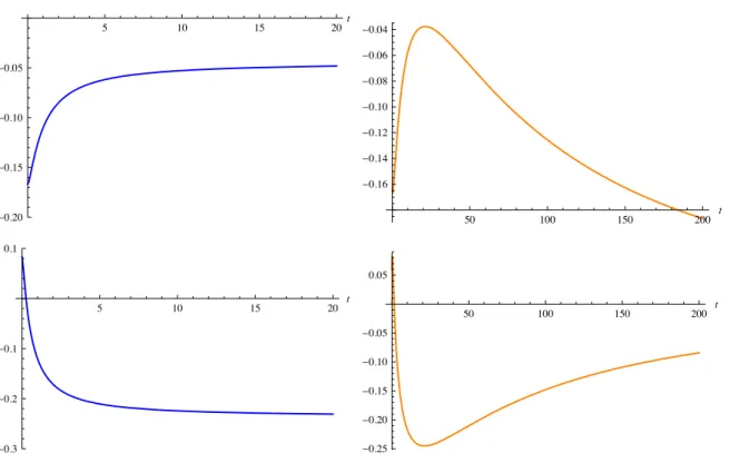
y x x x x F i i i x x F i i i x y x x x x F i i i x i x F i i i x ( ) 1 3 2, 2, , ( 1) 1 2, 1 2, 1 , , ( ) 1 3 2 3 1 2, 1 3 2 , 2 , 2 4 1 1 3 2 , 2 2, 2 , (B.34) i _i i i _i 1 4 3₄ 2 4 3₄ and so ⎡ ⎣ ⎢ ⎤ ⎦ ⎥ = = F x M x c M x w x w x y x y x ( ) ( ) , ( ) ( ) ( ) ( ) ( ) (B.35) i ij j 1 2 1 2

As we have discussed in the text, the physics of this simple model could be quite interesting, with a double crossing of the overlaps F_i2for some initial conditions. Moreover, as it is shown infigureB1, the absolute value of the determinant of M(x) is constant forx < 0 and nonvanishing. This indeed imply that this class of solution spans the wholeS2 = 0 subspace. More precisely, |det[M x( )] is indeed a (nonvanishing) constant in the connected domains| −∞

( , 0) , (0, 1) and (1, +∞), with jumps at the singular points of w₁ and w₂. The fact that, inside these domains, |det[M x( )] is a nonzero constant re| flects the unitarity of the quantum

time evolution, that implies + = F x₁( )2 F x₂( )2 nonvanishing constant, (B.36) or, equivalently = † M x M x( ) ( ) nonvanishing constant, (B.37) and therefore

|det(M x( )| =2 nonvanishing constant. (B.38)

References

[1] Calabrese P and Cardy J 2006 Time dependence of correlation functions following a quantum quench Phys. Rev. Lett. 96 136801

[2] Polkovnikov A, Sengupta K, Silva A and Vengalattore M 2011 Colloquium: nonequilibrium dynamics of closed interacting quantum systems Rev. Mod. Phys.83 863–83

[3] Calabrese P and Cardy J 2005 Evolution of entanglement entropy in one-dimensional systems J. Stat. Mech.

2005 P04010

[4] Chiara G D, Montangero S, Calabrese P and Fazio R 2006 Entanglement entropy dynamics of Heisenberg chains J. Stat. Mech. 2006 P03001

[5] Läuchli A M and Kollath C 2008 Spreading of correlations and entanglement after a quench in the one-dimensional Bose–Hubbard model J. Stat. Mech.2008 P05018

[6] Alba V and Heidrich-Meisner F 2014 arXiv:1402.2299

[7] Lewis H R J and Riesenfeld W B 1969 An exact quantum theory of the time-dependent harmonic oscillator and of a charged particle in a time-dependent electromagneticfield J. Math. Phys. 10 1458

[8] Perelomov A M and Popov V S 1969 Group-theoretical aspects of the variable frequency oscillator problem Theor. Math. Phys.1 275–85

[9] Kagan Y, Surkov E L and Shlyapnikov G V 1996 Evolution of a Bose-condensed gas under variations of the confining potential Phys. Rev. A54 1753–6

[10] Pitaevskii L P and Rosch A 1997 Breathing modes and hidden symmetry of trapped atoms in two dimensions Phys. Rev. A55 853–6

[11] Minguzzi A and Gangardt D M 2005 Exact coherent states of a harmonically confined Tonks–Girardeau gas Phys. Rev. Lett.94 240404

[12] Gritsev V, Barmettler P and Demler E 2010 Scaling approach to quantum non-equilibrium dynamics of many-body systems New J. Phys.12 113005

[13] Moore G and Read N 1991 Nonabelions in the fractional quantum hall effect Nucl. Phys. B360 362–96 [14] Sierra G 2000 Conformalfield theory and the exact solution of the BCS hamiltonian Nucl. Phys. B 572

517–34

[15] Sedrakyan T A and Galitski V 2010 Boundary Wess–Zumino–Novikov–Witten model from the pairing hamiltonian Phys. Rev. B82 214502

[16] Gaudin M 1983 La Fonction d’Onde de Bethe (Paris: Masson) (Engl. transl.) Gaudin M 2014 The Bethe Wavefunction (Cambridge: Cambridge University Press)

[17] Amico L, Falci G and Fazio R 2001 The BCS model and the off-shell Bethe ansatz for vertex models J. Phys. A: Math. Gen. 34 6425

[18] Ortiz G, Somma R, Dukelsky J and Rombouts S 2005 Exactly-solvable models derived from a generalized Gaudin algebra Nucl. Phys. B 707 421–57

[19] Urbaszek B, Marie X, Amand T, Krebs O, Voisin P, Maletinsky P et al 2013 Nuclear spin physics in quantum dots: an optical investigation Rev. Mod. Phys.85 79–133

[20] Latta C, Srivastava A and Imamoglu A 2011 Hyperfine interaction-dominated dynamics of nuclear spins in self-assembled InGaAs quantum dots Phys. Rev. Lett. 107 167401

[21] Childress L, Gurude Dutt M V, Taylor J M, Zibrov A S, Jelezko F, Wrachtrup J et al 2006 Coherent dynamics of coupled electron and nuclear spin qubits in diamond Science314 281–5

[22] Lidar D A, Chuang I L and Whaley K B 1998 Decoherence-free subspaces for quantum computation Phys. Rev. Lett. 81 2594–7

[23] Zanardi P and Rasetti M 1997 Noiseless quantum codes Phys. Rev. Lett.79 3306–9

[24] Lidar D A 2014 Review of decoherence free subspaces noiseless subsystems and dynamical decoupling Quantum Information and Computation for Chemistry (Advances in Chemical Physics vol 154) (arXiv:1208.5791)

[25] Di Francesco P, Mathieu P and Sénéchal D 1997 Conformal Field Theory (Berlin: Springer)

[26] Knizhnik V G and Zamolodchikov A B 1984 Current algebra and Wess-Zumino model in two dimensions Nucl. Phys. B247 83–103

[27] Babujian M 1993 Off-shell Bethe ansatz equations and N-point correlators in the SU(2) WZNW theory J. Phys. A: Math. Gen.26 6981

[28] Schechtman V V and Varchenko A N 1990 Hypergeometric solutions of Knizhnik–Zamolodchikov equations Lett. Math. Phys.20 279–83

[29] Nielsen A E B, Cirac J I and Sierra G 2011 Quantum spin Hamiltonians for the SU (2) k WZW model J. Stat. Mech.2011 P11014

[30] Nielsen A E B, Cirac J I and Sierra G 2012 Laughlin spin-liquid states on lattices obtained from conformal field theory Phys. Rev. Lett.108

[31] Whittaker E T and Watson G N 1996 A Course of Modern Analysis 4th edn (Cambridge: Cambridge University Press)

[32] Lima-Santos A and Utiel W 2006 Gaudin magnet with impurity and its generalized Knizhnik –Zamolodchi-kov equation Int. J. Mod. Phys. B20 2175–87

[33] Aomoto K and Kita M 2011 Theory of Hypergeometric Functions (Berlin: Springer)

[34] Yoshida M 1997 Hyper Geometric Functions, My Love: Modular Interpretations of Configuration Spaces (Braunschweig: Vieweg)

[35] Reshetikhin N and Varchenko A 1995 Quasiclassical asymptotics of solutions to the KZ equations Geometry, Topology, & Physics for Raoul Bott (Conference Proceedings and Lecture Notes in Geometry and Topology vol 9) pp 293–322