HAL Id: halshs-00348884
https://halshs.archives-ouvertes.fr/halshs-00348884v3
Submitted on 27 May 2010
HAL is a multi-disciplinary open access
archive for the deposit and dissemination of
sci-entific research documents, whether they are
pub-lished or not. The documents may come from
L’archive ouverte pluridisciplinaire HAL, est
destinée au dépôt et à la diffusion de documents
scientifiques de niveau recherche, publiés ou non,
émanant des établissements d’enseignement et de
New Prospects on Vines
Dominique Guegan, Pierre-André Maugis
To cite this version:
Documents de Travail du
Centre d’Economie de la Sorbonne
New Prospects on Vines
D
ominiqueG
UEGAN,Pierre André M
AUGIS2008.95
New Prospects on Vines
P.A. Maugis and D. Guegan
CES-MSE, Université Paris 1 Panthéon-Sorbonne,
106 boulevard de l’Hopital 75647 Paris Cedex 13, France
March 24, 2010
Abstract
In this paper, we present a new methodology based on vine copulas to estimate multivariate distributions in high dimensions, taking advantage of the diversity of vine copulas. Considering the huge number of vine copulas in dimension n, we introduce an efficient selection algorithm to build and select vine copulas with respect to any test T . Our methodology offers a great flexibility to practitioners to compute V aR associated to a portfolio in high dimension.
Keywords: Vine copulas - Multivariate copulas - Model Selection - V aR
1
Introduction
For almost ten years now, copulas have been used in econometrics and finance. They became an essential tool for pricing complex products, managing portfolios and evaluating risks in banks and insurance companies. For instance, they can be used to compute V aR (Value at Risk) and ES (Expected shortfall), Artzner et al. (1997). Moreover, copulas appear to be a very flexible tool, allowing for semi-parametric estimation, fast parameter optimisation and time varying parameters. These advantages make them a very interesting tool, although one major shortcoming is their use in high dimensions. Indeed, elliptical copulas can be expended to higher dimension, but they are unable to represent financial tail dependences (Patton, 2009), and the Archimedean copulas are not satisfactory as models to describe multivariate dependence in dimensions higher than 2 (Joe, 1997). In this paper we present a solution to this problem by using the vine copulas.
Recently, Aas et al. (2009) produced a seminal paper presenting a method to build high dimension copulas using pair-copulas as building blocks. Such decom-positions are called vine copulas. To build these copulas, the authors recursively
decomposed the dependence of the variables as done in Joe (1997) and Bedford and Cooke (2002, 2001). Another possible way to build multivariate copulas is to use nested copulas. This last notion is defined as follows: if C1(., .)and C2(., .)
are two bivariate copulas, then C1(C2(., .), .) is a trivariate nested copula. In
this paper we only consider vine copulas, which appear richer than nested cop-ulas for multivariate analysis, following (Berg and Aas, 2009) who show that nested copulas are less efficient than vine copulas to estimate densities and risk measures such as the V aR.
Our purpose is to build all possible vine copulas in order to capture as much information as possible from a dataset. Indeed, a practitioner aims to to find the vine copula that characterises correctly the behavior of the dataset under study: we call this true copula C0. However finding C0 is almost impossible
for any real dataset. On the other hand, a vine copula could be described as a decomposition of an n-variate vector’s density using bivariate copula densities as building blocks. Such vine decomposition is not unique, and many different vine copulas exist in each dimension. Through an example in Section 4 we show that, given a dataset, each vine decomposition estimates specific dependence between the variables.
This result highlights the importance of defining a strategy to find the vine cop-ula that is closest to the true copcop-ula C0 according to any criterion retained by
the practitioner. To do so we generated a large number of vine copulas using a simple algorithm that produces N =n!
2 ∏ n−3
i=1 i! different vine copulas in
dimen-sion n. Previously cited papers use n! vine copulas, but as our purpose is to find a copula closest to the copula C0, increasing the number of vine copula under
consideration is crucial. The size of the set of possible vine copulas necessitates a computationally efficient selection algorithm. We present an algorithm that has the advantage of selecting the best vine copula within a set of vine copulas according to any criterion chosen by the practitioner without the requirement of having to test all the copulas. This algorithm is based on an underlying lattice structure inside the set of vine copulas.
The paper is organised as follows: in Section 2, we introduce a new method to build vine copulas. Section 3 provides some characteristics of vine copulas that motivated our work. In Section 4, we describe the model selection procedure, relying on a lattice structure on the set of vine copulas. Section 5 presents a numerical application and Section 6 concludes.
2
The Vine Set
In this section, we introduce a new algorithm to build vine copulas. It consists of a step-by-step factorisation of the density function in a product of bivariate copulas. Our approach is different from the methods developed by Bedford and
Cooke (2002, 2001) and is not related to them in any obvious way. Indeed, in Bedford and Cooke (2002, 2001) vine copulas are introduced as decomposition of the multivariate random vector density based on a type of graph structure called "vines", from which comes their denomination. Our approach has the advantage of being able to coherently describe a large set of vine copulas – N in dimension n – while also being a simple recursive algorithm.
2.1
Formula
Let us consider a vector X = (X1, X2, . . . , Xn)of random variables characterised by a joint distribution function FX that we assume has a density function fX.
We introduce the following notations:
• X−α= (X1, . . . , Xα−1, Xα+1, . . . , Xn)is the set of variables except the α-th. • We denote fαthe density of Xα. In the same fashion fα∣β is the density of
(Xα∣Xβ), f−α is the density of X−α and fα∣−β is the density of Xα∣X−β.
• cα,β∣γ=cXα,Xβ∣Xγ(FXα∣Xγ(Xα∣Xγ), FXβ∣Xγ(Xβ∣Xγ))is the copula density of (Xα, Xβ∣Xγ)as defined in Sklar (1959)’s theorem. Similarlycα,β∣−(α,β)= cXα,Xβ∣X−(α,β)(FXα∣X−(α,β)(Xα∣X−(α,β)), FXβ∣X−(α,β)(Xβ∣X−(α,β))).
Our objective is to compute c1,...,n, the copula density associated with the vector
X. This will be done by factorizing fX in the following form:
fX= ∏
i=1,...n
fi⋅c1,...,n.
By construction for n = 2 we have: fα,β =fα.fβ.cα,β. Using this property we
consider the following factorisation of the joint density fX:
∀α, β ∈ {1, . . . , n}2, α ≠ β fX=f−α.fα∣−α=f−α. fα,β∣−(α,β) fβ∣−(α,β) = f−α. fα∣−(α,β).fβ∣−(α,β) fβ∣−(α,β) .cα,β∣−(α,β) = f−α.f−β f−(α,β).cα,β∣−(α,β). (1) Formula (1) allows the computation of an n-variate density with a bivariate copula, two (n − 1)-and one (n − 2)-variate densities. Using this factorisation recursively, insuring that the denominators cancel at each step, we produce a factorisation of the n-variate density as a product of univariate and bivariate
copula densities. Using this algorithm we can produce all N possible vine cop-ulas (Napoles, 2007)1,2.
2.2
Example
In this example, we illustrate the unwinding of the previous algorithm for n = 4, providing the joint density function f1,2,3,4. Our aim is to compute c1,2,3,4:
the joint copula density. We describe the two steps of the algorithm using the previous notations. • First step: f1,2,3,4= f1,2,3.f1,2,4 f1,2 .c3,4∣1,2= f1,2,3.f1,2,4 f1.f2.c1,2 .c3,4∣1,2. (2)
• Second step: we apply the relationship (1) to the densities f1,2,3and f1,2,4:
f1,2,3=f1,2.f1,3 f1 .c2,3∣1=f1.f2.c1,2.f1.f3.c1,3 f1 .c2,3∣1=f1.f2.f3.c1,2.c1,3.c2,3∣1, (3) and f1,2,4=f1,2.f2,4 f2 .c1,4∣2=f1.f2.c1,2.f2.f4.c2,4 f2 .c1,4∣2=f1.f2.f4.c1,2.c2,4.c1,4∣2. (4)
By merging formulas (2),(3) and (4), we obtain the following factorisation: f1,2,3,4=f1.f2.f3.f4.c1,3.c1,2.c2,4.c2,3∣1.c1,4∣2.c3,4∣1,2. (5)
We have now factorised the density f1,2,3,4 into a product of four univariate
densities and six bivariate copula densities. By construction, this means that the copula density of (X1, X2, X3, X4)can be factorised as follows:
c1,2,3,4=c1,3.c1,2.c2,4.c2,3∣1.c1,4∣2.c3,4∣1,2.
The unwinding of this algorithm can yield other vine copulas if other param-eters are used. For instance the copula density c1,2,3,4 has also the following
decomposition:
c1,2,3,4=c2,3.c3,4.c1,4.c2,4∣3.c1,3∣4.c1,2∣3,4.
1N is the number of "vine" type graphs with n nodes, which is also the number of vine copulas (see Bedford and Cooke (2002, 2001)). The proof of the formula relies heavily on the graph structure of vines.
2Our algorithm can produce more varied decomposition, however we do not consider them as they are not efficient estimators, Bedford and Cooke (2002, 2001).
3
The Vine Copula Estimator
Using the previous algorithm for an n-variate density, we can construct the N different vine copulas in dimension n. In the following, using a real dataset as example, we show how each vine copula can yield different representations of the same dataset. We proceed in the following way.
We estimate two different trivariate vine copulas from the same dataset and compare the tail dependence of the two estimated densities by observing in which quadrant of [0, 1]3 the densityes evolves3. The dataset is the daily
Mor-gan Stanley evaluation of the French, German and British price indexes from 01/01/06 to 01/12/08 (Datastream). We denote them respectively as X, Y and Z. In a first step, for X, Y and Z we estimate separately GARCH(1, 1) models using pseudo-maximum likelihood methods, Ghysels et al. (1995). In a second step, using the residuals, we estimate the parameters of the vine copula using maximum likelihood, Chen and Fan (2006). For each bivariate copula in the estimation procedure, we select among the Gaussian, Student, Clayton and Gumbel copula, the one with higher likelihood. We choose these copulas because they characterise the main features detected in economic and financial time-series (Patton, 2009)4. In Figure 1, we plot the estimated copulas with
uni-form margins in three cases: (X, Y ∣z = 0.1), (X, Y ∣z = 0.5) and (X, Y ∣z = 0.9) (from left to right).
By examining Figure 1, we observe that the two vine copulas describe different tail dependences. According to the first vine copula there is strong upper tail dependence (top-right plot) but no lower dependence (top-left plot). However the second vine copula describes strong lower tail dependence (bottom left plot) but no upper tail dependence (bottom right plot). This difference in terms of tail dependence is solely caused by the vine copula, since in both cases we used the same estimation procedure and the same dataset.
Taking this fact into account and to attain our purpose of finding the copula that is closest to the true one C0 according to a criterion chosen by the practitioner,
we decided to consider the whole set of possible vine copulas. However, as there are N different vine copulas in dimension n, estimating and testing all of them is computationally intractable, thus we needed to develop an efficient search strategy. In the next section, we describe such an algorithm using a lattice structure. We denote T the test retained by the practitioner to make the selection.
3The two copulas used are: V ine 1= c1,2.c1,3.c2,3∣1and V ine 2= c1,3.c2,3.c1,2∣3 4All computations are done in M atLab.
First trivariate Vine
Second trivariate Vine
Figure 1: Two vines estimated on the same data set: slices at z = 10%, 50%, 90%
4
Model Selection
In this section, we describe the search algorithm that finds the set of vine copulas accepted by the test T among all possible vine copulas. To this end, we introduce a lattice which is a partial order on the set of vine copulas. We proceed in two steps: we first introduce lattice theory and the implemented lattice structure, and then we describe the search algorithm. We illustrate our approach with an example in dimension n = 3.
Lattice Theory A lattice is a set and a partial order. A partial order is a binary relation, for instance denoted ≤, that is reflexive, antisymmetric and transitive, i.e for all a, b, and c, we have that:
• a ≤ a (reflexivity)
• if a ≤ b and b ≤ a then a = b (antisymmetric) • if a ≤ b and b ≤ c then a ≤ c(transitive)
For instance the set R with binary relation ≤ is a lattice.
The lattice structure we build from the set of all possible vines is based on increasing independence hypotheses. For instance, in the trivariate case when
the random variables (X1∣X2) and (X3∣X2) are independent, the vine copula c1,2,3 =c1,2.c2,3.c1,3∣2 becomes c1,2,3 =c1,2.c2,3. Thus, we will consider c1,2,3 = c1,2.c2,3 as being a vine copula and insert it into the lattice structure5.
In dimension three we get the following lattice structure:
"1" is the root of the lattice, and the arrow points from a general vine copula to a more specific one. We say that the vine copula "c1,3" is more general than the
vine copula "c1,2.c1,3" because the former vine copula defines a simpler relation
between the variables and requires fewer parameters than the latter one. This kind of specification of the vine copulas is different from that introduced by Czado et al. (2009), which is based on a Bayesian selection framework.
We proceed now to construct the search algorithm based on the lattice structure in the general case. The use of lattices to organise large sets of models is not new, but lattice selection has never been used on vine copulas. Gabriel (1969) developed the principles and provided the theoretical groundwork for such a method. It relies on two tools, first a test T to decide whether a model is accepted or rejected6, second on the rule of coherence: "one ought not to accept
a model while rejecting a more general model." When we apply the test T on a model, if the null of the model being the true model is retained then we accept all generalisations of this model, and if the null is rejected we reject all specifications of this model. In our case, the term "model" refers to vine copulas, and the rule of coherence could be restated as follows: "the gain in increased specification does not compensate for the loss of requiring more parameters." We now develop the search algorithm based on the rule of coherence. Within the set of models, it selects the subset of all possible vine copulas composed of the most complex models accepted by a test T :
1. We randomly build a set S of possible models and classify them into two sets according to the test T : A, the accepted models and R, the rejected models.
2. i If A ≠ ∅: let DAbe the set composed of the most complex models that
are not in A or R. If DA= ∅we stop; otherwise we test with T the models in DA. If we do not retain any models, we stop. Otherwise,
we update A and R accordingly and iterate.
ii If A = ∅: let DR be the set composed of the most simple models
that are not in A or R. If DR= ∅we stop; otherwise we test with T the models in DR. If we accept all models, we stop. Otherwise, we
update A and R accordingly and iterate.
5This imply that the number of copulas we consider is greater than N .
6We do not specify T in this section, and instead describe the procedure for any test chosen by the practitioner, but we specify a possible test in Section 5.
Edwards and Havranek (1987) study a similar algorithm and prove that the algorithm reaches its purpose efficiently. This means that given a set of models of size p it will only require o(log(p)) steps to find the optimum.
We give a step-by-step illustration of how the previous algorithm could unwind in the case of our trivariate example. Let X be a trivariate dataset and T a test. First, two vine copulas are selected randomly to be tested, c1,3.c2,3 and
c1,2.c1,3. The former one is accepted (solid line) while the latter one is rejected
(in black) by the test T , as can be seen in the upper left diagram.
The consequence of c1,3.c2,3being accepted according to the rule of coherence is that
three more vine copulas are accepted: 1, c2,3 and c1,3(dashed lines in the upper right
diagram). Similarly, the consequence of c1,2.c1,3 being rejected is that c1,2.c1,3.c2,3∣1
is also rejected (in grey in the upper right diagram). The next step of the algorithm is to test using T the most complex vine copulas that are not accepted or rejected: c1,3.c2,3.c1,2∣3and c1,2.c2,3.c1,3∣2 (underlined in the upper right diagram). The former
copula is refused, and the latter one is accepted (in the lower left diagram) by the test T . By the rule of coherence, we accept: c1,2 and c1,2.c2,3. In summary, the
research algorithm keeps the most complex among the accepted vine copulas, which is c1,2.c2,3.c1,3∣2 (double lines in the lower right diagram).
The advantage of this lattice structure is that it presents a high connectivity inside the set of all possible vine copulas. For instance, c1,2is connected directly or indirectly to
five other vine copulas. This means that each step of the algorithm is very useful for the search, because it allows us to accept or reject many other copulas by using the rule of coherence.
5
Application to the CAC40 index
Here we estimate the joint density of the five main assets composing the CAC40, the French leading index, using the methodology described above, and we use this estimated joint density to compute the V aR of a portfolio composed of the five assets. The dataset is taken from Datastream, daily quotes from Total, BNP - Paribas, Sanofi - Synthelabo, GDF-Suez and France Telecom from 25/4/08 to 21/11/08. This period is marked by the 2008 crisis, and our purpose is to test the resilience of our model to this shock and change of regimes. We estimate the parameters and select the vine copula based on the data ranging from 25/4/08 to 9/12/08, while the V aR is computed from the remaining dates. The portfolio we consider is as follows: Total (33%), BNP - Paribas (20%), Sanofi - Synthelabo (20%), GDF-Suez (14%) and France Telecom (13%).
For each dataset a GARCH(p, q) process is selected using the AIC criterion (Akaike, 1974) and estimated using pseudo likelihood. On the residual we estimated the vine copula parameters using maximum likelihood. The parametric copula families used in this exercise are the Clayton, Gumbel, Student and Gaussian copulas.
Anderson-Darling (A-D) type test modified for use with copulas in high dimension. It is described in Chen et al. (2004) and shown through Monte-Carlo simulation of possessing significant power even in high dimension. We recall that this test associates to each estimated density a χ2 sample. A complete presentation of the test is detailed in the Annex.
In dimension five, the lattice structure contains 8536 different vine copulas. Using our lattice-based algorithm in order to select the best vine copula according to the A-D test, we only needed to test 1423 vine copulas (less that 17% of them). In fine, the retained vine copula is7:
c1,2,3,4,5=c2,5.c4,5.c1,3.c1,5.c1,5∣4.c1,2∣5.
The fact that this vine copula was selected imply that the vines copulas presented in Aas et al. (2009) were rejected by the test, and hence were unable to represent the dependence between the five assets properly. This example shows the necessity of using the whole set of vine copulas for times series applications.
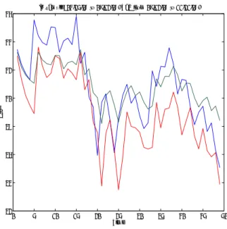
Our final objective is to use this estimated vine copula density to compute the 10% V aR8. We computed it from 9/12/08 to 21/11/08 using Monte-Carlo based integration and optimisation, see Figure 2. We compared it to a univariate GARCH(p, q) model-based estimate of the V aR computed directly on the portfolio value time series. To discriminate between the two approaches, we use the Kupiec test (Kupiec, 1995). The Kupiec statistic is the number Q of time the out-sample time-series is below the predicted 10% V aR. Under the null of the prediction being a true 10% V aR the sampling distribution of the statistic follows a binomial distribution of parameter 0.1. In our example the vine copula-V aR has a p-value of 0.96 for the Q statistic, so it is accepted as a true V aR, while the GARCH-V aR has a p-value of 0.00 and is rejected according to this test9. Nevertheless, the vine copula approach fails to predict the major drop during the crisis, but the prediction remains solid before and after the crisis. These results make the vine copula methodology we described an interesting approach for risk management in order to estimate the multivariate (n > 2) density of a portfolio and to compute its associated V aR.
6
Conclusion
In this paper, we estimated multivariate distributions in high dimensions using a new vine copula-based approach that builds upon the work of Aas et al. (2009) by taking advantage of the diversity of vine copulas. We introduced an algorithm using a large number of vine copulas from which we were able to retain the "best" one according to a predefined test T , using a lattice structure, which makes the research simple and fast. The methodology we developed offers great flexibility for the practitioners in
7The computation took one hour on a 1.5Ghz processor computer.
8Given a random variable X, the 10% V aR of X is the value V aR(X) such that: P(X < V aR(X)) = 0.1.
0 5 10 15 20 25 30 35 40 45 50 32 34 36 38 40 42 44 46 Time Price
In sample: 04/25/08 to 09/12/08. VaR from 09/12/08 to 11/21/08.
Figure 2: In Blue: The CAC40, In Red: Vine VaR Estimation, In Green: GARCH VaR Estimation.
terms of the choice of the set of vine copulas, choice of bi-variate copulas, usefulness of the lattice structure, and the test T for the selection procedure.
It appears necessary to have a great number of vine copulas to be able to take into account the most important features of the dataset to be analysed: indeed, through a simple example we have highlighted the importance of finding the vine copula that takes into account most of the information contained in the dataset, particularly the behaviour of the tails. Finally, the V aR computation based on our methodology provides interesting results compared with the classical parametric approach. However, some questions remain. First is the problem of devising a test to decide whether a vine copula represents a dataset dependence correctly or not. Chen et al. (2004) and Chen and Fan (2006) produced interesting tests, but for an optimum use of vine copulas a simpler and more efficient test needs to be built. Another question concerns the quality of the estimates, on which we did not focus in this paper. Instead, we applied a classical maximum likelihood estimation approach as developed for instance in Aas et al. (2009) to estimate the vine copula parameters. Results on the efficiency of the estimates have to be established. We address this question in a companion paper, Guégan and Maugis (2009).
7
Acknowledgment
This work has already been presented at the Sorbonne Finance Seminar (Paris, France, 2009), at the MIT Econometric Seminar (Cambridge, USA, 2009) and at the Interna-tional Symposium in ComputaInterna-tional Economics and Finance (Sousse, Tunisia, 2010). We thank the participants of the seminars and our reviewers for their helpful com-ments. All remaining errors are still ours. P.A. Maugis thank Arun Chandrasekhar, Victor Chernozhukov, Matthieu Latapy and Miriam Sofronia for their helpful com-ments.
References
Aas, K., Czado, C., Frigessi, A., Bakken, H., 2009. Pair-copula constructions of mul-tiple dependence. Insurance: Mathematics and Economics 44, 182–198.
Akaike, H., 1974. A new look at the statistical model identification. IEEE Trans. Automatic Control AC-19, 716–723.
Artzner, P., Delboen, F., Eber, J., Heath, D., 1997. Thinking coherency. Risk 10, 68–71.
Bedford, T., Cooke, R., 2001. Probability density decomposition for conditionally dependent random variables modeled by vines. Annals of Mathematics and Artificial Intelligence 32, 245–268.
Bedford, T., Cooke, R., 2002. Vines: A New Graphical Model for Dependent Random Variables. The Annals of Statistics 30 (4), 1031–1068.
Berg, D., Aas, K., 2009. Models for construction of multivariate dependence. Forth-coming in The European Journal of Finance.
Chen, X., Fan, Y., 2006. Estimation of copula-based semi-parametric time series mod-els. Journal of Econometrics 130, 307–335.
Chen, X., Fan, Y., Patton, A., 2004. Simple Tests for Models of Dependence Between Multiple Financial Time Series, with Applications to U.S. Equity Returns and Ex-change Rates. London Economics Financial Markets Group Working Paper (483), london, UK.
Czado, C., Gartner, F., Min, A., 2009. Analysis of Australian electricity loads using joint Bayesian inference of D-Vines with autoregressive margins. Zentrum Mathe-matik Technische Universitat Munchen: Working Paper Munchen, Germany. Edwards, D., Havranek, T., 1987. A Fast Model Selection Procedure for Large Families
of Models. Journal of the American Statistical Association 82 (397), 205–213. Gabriel, K. R., 1969. Simultaneous Test Procedures - Some Theory of Multiple
Com-parisons. Annals of Mathematics Statistics 40 (1), 224–250.
Ghysels, E., Harvey, A., Renault, E., 1995. Stochastic volatility. Papers, Toulouse -GREMAQ.
Guégan, D., Maugis, P. A., 2009. Dealing With Vines Isues. Work in Progress. Joe, H., 1997. Multivariate Models and Dependence Concepts. Chapman & Hall,
Lon-don, UK.
Kupiec, P. H., 1995. Techniques for verifying the accuracy of risk measurement models. Board of Governors of the Federal Reserve System (U.S.), Washington (95-24). Napoles, O. M., 2007. Number of vines. 1st Vine Copula Workshop Working Paper. Patton, A., 2009. Handbook of Financial Time Series. Springer Verlag, Ch.
Copula-Based Models for Financial Time Series, pp. 767–781.
Sklar, A., 1959. Fonctions de répartition à n dimensions et leurs marges. Publications de l’Institut de Statistique de L’ Université de Paris 8, 229–231.
8
Annex
8.1
The modified Anderson-Darling test, Chen et al. (2004)
The test is the following: we are testing the null hypothesis H0against the alternative
hypothesis H1:
H0∶P r(C(U1, . . . , Un) =C0(U1, . . . , Un)) =1 H1∶P r(C(U1, . . . , Un) =C0(U1, . . . , Un)) <1
where C is the true copula and C0 the estimated copula. We define {Zi}i<n and W as:
Zi=F (Ui∣U1, . . . , Ui−1)and W =
n
∑
1
[Φ−1(Zj)]2,
where Φ is the standard normal distribution function. Then W follows a χ2d
distri-bution; our test will be based on this result. For this purpose we use the univariate boundary kernel Kh(x, y) Kh(x, y) = ⎧ ⎪ ⎪ ⎪ ⎪ ⎨ ⎪ ⎪ ⎪ ⎪ ⎩ k(x−yh )/ ∫−1x h k(u)du if x ∈ [0, h) k(x−yh ) if x ∈ [h, 1 − h] k(x−yh )/ ∫−1xhk(u)du if x ∈ (1 − h, 1]
in which k(⋅) is the quartic kernel: k(u) = 15 16(1 − u
2
)21∣u∣<1 and h is fixed using the
rule of thumb: h = √
V ar(W )n−1/5. Then we define gW as a kernel estimation of the
inverse density of W : gW(ω) = 1 n.h T ∑ t Kh(ω, Fχ2 d(Wt))
Finally the test is based on the statistics Jn:
Jn= ∫
1
Then under the null we have that: Statn=(nh 1/2 Jn−rn) σ →N (0, 1) in distribution. Where: rn=h1/2 [(h−1−2)∫−11 k2(ω)dω + 2∫01∫−1z kz2(y)dydz] σ2=2∫−11[∫−11 k(u + v)k(v)dv] 2 du kz(y) = k(y)/∫ z −1k(u)du