Deterministic chaos in an experimental economic system

WORKING

PAPER

ALFRED

P.

SLOAN

SCHOOL

OF

MANAGEMENT

DETERMINISTIC CHAOS

IN

AN EXPERIMENTAL ECONOMIC

SYSTEM

John

D.

Sterman

July, 1988

WP #2040-88

MASSACHUSETTS

INSTITUTE

OF

TECHNOLOGY

50

MEMORIAL

DRIVE

CAMBRIDGE,

MASSACHUSETTS

02139

j;m

John

D.

Sterman

MIT.

LIBRARIES

"3

1 6 1988

Deterministic

Chaos

in

an

Experimental

Economic

System

John D.

Sterman

Massachusetts Institute of

Technology

Sloan School of

Management

Cambridge,

MA

02139

July 1988

The

contributions and

comments

of Richard

Day,

Christian

Kampmann,

Edward

Lorenz, Ilya Prigogine,

James

Ramsey, Rebecca

Waring, and particularly Erik

Abstract

An

experiment with a simulated

macroeconomic

system demonstrates that the

decision-making processes of agents can

produce

deterministic chaos. Subjects

managed

capital investment in a simple multiplier-accelerator

economy.

Performance, however,

was

systematically suboptimal.

A

model

of the subjects' decision rule is proposed and related to

priorstudies of

dynamic

decision making.

Econometric

estimates

show

the

model

is an

excellent representation of the actual decisions.

The

estimated rules are then simulated to

evaluate the stability of the subjects' decision processes.

While

the majority of the estimated

rules are stable, approximately

40%

yield a variety of

dynamics

including limit cycles, period

multiples, and chaos. Analysis ofthe parameter space reveals a

complex

bifurcation

structure. Implications for

models

of

human

systems

and

experimental studies of

economic

dynamics

are explored.

1. Introduction: coupling nonlinear

dynamics and

experimental

economics

Recent

work

in the physical sciences has

shown

deterministic chaos to be a

common

mode

of behavior in

dynamic

systems, thus stimulating the search for chaos

and

other highly

nonlinear

phenomena

in

human

systems. Indeed, there has been a near explosion of

models

and

empirical studies

which

seek to

show

the relevance ofnonlinear

dynamics

and chaos in

social

and

economic

settings. Several journals have devoted special issues to chaos and

models

ofnonlinear, disequilibrium

dynamics

in

human

systems.^ This robust literature can

be divided roughly into (1) theoretical

models

of nonlinear dynamics, and (2) empirical

studies

which

seek evidence of chaos in

economic

data.

Theoretical studies include the

work

of

Day

(1982),

Dana

and

Malgrange

(1984),

Grandmont

(1985),

Rasmussen

and

Mosekilde

(1988), Stutzer (1980),

and

many

others (see

note 1).

A

survey of these studies suggests the following generalizations. First,

many

standard models, both micro-

and macroeconomic,

when

modified to include realistic

nonlinearities, can be

shown

to contain regimes ofchaos and other nonlinear

phenomena

such

as mode-locking, period multiples, and quasiperiodicity.

Benhabib and

Day's (1981) studies

of such simple

models

lead

them

to "expect the possibility oferratic [chaotic] behavior fora

wide

variety of

dynamic economic models

involving rational decision-making with feedback."

Subsequent

work

has borne out this conjecture

-

the possibility ofchaos does not

seem

to

depend on

particular behavioral assumptions but

on

more

fundamental properties.

However,

most models

ofnonlinear

dynamics

have been purely theoretical, and have not involved

econometric estimation of the parameters.

The

few

exceptions

have found

the estimated

parameters lie well outside the chaotic regime, e.g.

Candela

and Gardini (1986)

and

Dana

and

Malgrange

(1984).

As

Day

and

Shafer (1985, 293) note,

"Whether or not

we

can construct empirical models that offerconvincing explanation ofreal world

macro activity [in terms of deterministic chaos] is an open question: most economists would probably

agree that

we

are as yet quite far from a definitive answer to it. What

we

know now...is that among

the empirical phenomena that

we

can hope to explain...are stochasticlike fluctuations in economic data.

Moreover,

we

need not expect thatexotic assumptions or bizarre model structures will be required"

D-3976

The

relative simplicity and theoretical focus of the

models

is entirely appropriate to the

early exploration of

new

concepts and analytical tools.

However,

the theoretical

work

to date

leaves

unanswered

questions about the relevance of these models.

Can

chaos arise

from

the

behavior ofactual agents?

Do

the chaotic regimes in the

models

lie in the realistic region of

parameter space, or are they mathematical curiosities unrealized in actual

economic

systems?

The

empirical literature has sought to

answer

these questions

by

searching for

evidence of chaos in

economic

data. This literature is notable for the clever adaptation of

techniques originally applied in physical settings, such as the

Takens

(1985)

method

for

recovering low-dimensional attractors

from

a single time series, the Wolf, Swift, Swinney,

and

Vastano (1985) technique forestimation of

Lyapunov

exponents

from

experimental time

series, and the Grassberger-Procaccia (1983) correlation dimension.

The

results are

tantalizingly suggestive but inconclusive.

Brock

(1986) demonstrates a

method

to test the

hypothesis of chaos in

economic

data against explicit alternative hypotheses, but finds "that

there is not

enough

information available in U.S. real

GNP,

real gross private domestic

investment,

and

Wolfer's sunspot series...to reject the null hypothesis that...[these series

were] generated

by

an

AR(2)

process."

Chen

(1988) and

Bamett and

Chen

(1988),

however, find evidence of

low

dimensional strange attractors in

some

but not all measures of

U.S.

monetary

aggregates. Their conclusions are tempered, however,

by

uncertainties such

as the sensitivity of the

methods

used to the

number

of data points, the

number

of points per

orbit, the

(unknown) magnitude

and statistical character of process noise, and the

(unknown)

magnitude

and character of

measurement

error

[Ramsey and

Yuan

(1987)].

Brock

(1986, 192) concludes "It is not

enough

when

you

are

working

with short data sets to report

low

dimension and positive

Lyapunov

exponents to

make

the case for deterministic chaos in your

data" (emphasis in original).

Ramsey,

Sayers, and

Rothman

(1988) have identified

significant biases in calculations ofcorrelation _{dimension caused by} small sample size and conclude "that while there is abundant evidence for the presence ofnonlinear stochastic

attractors of the type that have been discovered in the physical sciences."

The

prevalence ofchaos in the

models

but

low

power

of aggregate statistical tests

motivates a

complementary

approach based

on

laboratory experiments with simulated

eco-nomic

systems.

The

pioneering

work

of Smith (1982, 1986), Plott (1986),

and

others has

demonstrated that

many

economic

theories can be successfully tested in the laboratory. This

paper applies these techniques to the investigation of chaos in

economic

systems. I report

the results of an experiment with a simulated

macroeconomic

system, specifically a

multi-plier-accelerator model. In the experiment, subjects play the role of

managers

of the

capital-producing sector of an

economy.

Each

time period they

must

make

a capital investment

decision.

The

task ofthe agents is to

manage

a

complex

dynamic

system in disequilibrium, a

system with time lags, multiple feedbacks, and nonlinearities. I

show

that the behavior ofthe

subjects is systematically suboptimal, suggesting the use of a

common

heuristic for decision

making.

A

model

ofthe subjects' decision rule is proposed.

The

model

is well

grounded

in

the literature ofeconomics, psychology, and behavioral decision theory.

Econometric

estimation

shows

the decision rule explains the agents' behavior well.

Next

the estimated

decision rules are simulated, and it is

shown

that approximately

40%

ofthe agents produce

unstable behavior, including chaos.

The

parameter space of the system is

mapped

and

shown

to contain a

complex

bifurcation structure.

Thus

experimental evidence is

adduced

that the

actual decision processes of agents in a

common

economic

context can produce chaos.

Limitations of the method, implications,

and

suggestions for future research are discussed.

2.

The Model

The

experiment is based

on

a simple

model

of the capital investment accelerator and

is fully described in

Sterman

(1988a).

The

model

creates a two-sector

economy

with a

capital producing and

goods

producing sector.

The

focus is the capital investment accelerator.

Goodwin

(1951, 4) notes that the traditional acceleration principle

assumes

...that actual, realized capital stock is maintained at the desired relation with output.

We

know in

reality that it is seldom so, there being now too much and

now

too little capital stock. For this there

D-3976

4

industry....At the otherextreme there is an even more inescapable and effective limit. Machines, once made, cannot be unmade, so that negative investment is limited to attrition from wear.. ..Therefore

capital stock cannotbe increased fast enough in the upswing, nor decreased fastenough in the

downswing, so that atone time we have shortages and rationing of orders and at the other excess

capacity with idleplants and machines.

A

single factor ofproduction (capital plant and equipment) is considered.

The

model

includes,

however, an explicit representation ofthe capital acquisition delay (construction lag) and the

capacity ofthe investment

goods

sector.

As

a result, orders for

and

acquisition of capital are

not necessarily equal, and at any

moment

there will typically be a supply line ofcapital under

construction. For simplicity, the

demand

for capital of the goods-producing sectoris

exogenous, and there is

no

representation ofthe

consumption

multiplier.

The

model

allows forvariable utilization of the capital stock.

Thus

production

P

is the

lesser ofdesired production

P*

orproduction capacity C. Capacity is proportional to the

capital stock, with capital/output ratio k:

Pt

=

MIN(P*„Ct)

(1)

Ct = Kt/K. (2)

The

capital stock of the capital sector is

augmented

by acquisitions

A

and diminished

by

depreciation D.

The

average lifetime ofcapital is given by x:

Kt^l

=Kj

+

(Aj-Dj)

(3)

Dt =

Kt/T. (4)

The

acquisition of capital by both the capital and

goods

sectors

(A

and

AG)

depends on

the

supply line ofunfilled orders each has accumulated (the backlogs

B

and

BG)

and the fraction

ofthe backlog delivered that period (J) (the suffix 'G' denotes a variable ofthe

goods-producing sector):

A,

= _{Bf4)t (4)}

AGt

=

BGt•(^, (5)

<l>t

=

Pt/P*t (7)

P*t = Bi

+BGt.

(8)

unless the capital sector is unable to produce the required amount. Ifcapacity is insufficient

so that

P*>C,

<t)<l

and

shipments to each sector fall in proportion to the shortfall.

Note

that

the formulation for

<J) implies that

A+AG=P

at all times, ensuring that output is conserved.

The

explicit representation ofthe construction supply line and the constraint

on

production

mean

that the lag in acquiring capital

may

be variable. It is easily

shown

that the average

capital acquisition lag A=l/()). Normally, <\>=\ and

A=l

period. Ifcapacity is inadequate,

however, <\> falls

and

A

lengthens as the backlogs of unfilled orders

grow

relative to output.^

The

supply lines of unfilled orders foreach sector

B

and

BG

are

augmented

by orders

for capital placed

by

each sector and emptied

when

those orders are delivered:

Bui

=Bt

+

(Ot-Ai)

(8)

BGt+i

-

BGt

+

(OGfAGt).

(10)

Orders placed by the

goods

sector are an

exogenous

input to

which

the subjects of the

experiment

must

respond

by

ordering an appropriate

amount

ofcapital for their

own

use:

OGt

= exogenous

(11)

Oj =

determined by subject. (12)

Equations (1)-(12) thus define a third-order nonlinear difference equation system.

The

system has the interesting property that the nonlinear capacity utilization function ofeq.

(1) divides the system into

two

distinct regimes, (^=\

and

(}><1. Furthermore, the equilibrium

point

P* =

C

lies exactly at the boundary. Considering each region in turn reveals interesting

properties of the

open

loop system.

When

P*=P<C,

0=1,

and

the system is linear:

Kl+1

Bui

BGt.i

Bt

BGi

1 1

OG,

(13)

Excess capacity implies each sector receives the quantity ordered after

one

period.

Note

that

the system in this

regime

is always stable.

The

capital stock is controllable via orders

O

(it

D-3976

there is excess capacity, the goods-producing and capital-producing sectors are decoupled.

When

capacity is inadequate, however,

P*>P=C,

(})<1,

and

the system is nonlinear.

Linearizing the system around the operating point (K, B,

BG)

anddefining

P*

=

B-i-BG

and

^=

(K/K)/P* yields

l-i.-L

T kP*

B

kP*

BG

kP* <t>

=^

P* p* P* P* p*

Kt

seminal

work

of

Smith

(1982) and Plott(1986).

The

experimental protocol used here is

described in

Sterman

and

Meadows

(1985) and

Sterman

(1987, 1988a).

A

continuous time

version ofthe

model

is developed and analyzed in

Sterman

(1985).

For

the experiment it has

been converted to discrete time. Simulation

and

formal analysis confirm that the conversion

to discrete time does not alter the essential

dynamics

of the system [Rasmussen,

Mosekilde

and

Sterman

(1985),

Sterman

(1988b)].

The

experiment is

implemented on

IBM

PC-type

microcomputers.

A

'game board' is displayed

on

the screen and provides the subjects with

perfect information. Colorgraphics and animation highlight the flows oforders, production,

and

shipments to increase the transparency of the structure (figure 1).^

No

overt time

pressure

was

imposed.

The

parameters (k=1 and

x=10)

were

chosen to

minimize

the

computational burden

imposed on

the subjects, while remaining close to the original values.

The

subject population

(N=49)

consisted of

MIT

undergraduate, master's

and

doctoral

students in

management

and

engineering,

many

with extensive exposure to

economics and

control theory; scientists

and

economists

from

various institutions in the

US,

Europe, and the

Soviet Union;

and

business executives experienced in capital investmentdecisions including

several corporate presidents

and

CEOs.

Subjects are responsible foronly

one

decision

-

how much

capital to order.

The

goal

ofthe subjects in

making

these decisions is to

minimize

total costs.

The

cost function or

score

S

is defined as the average absolute deviation

between

desired production

P*

and

production capacity

C

over the

T

i>eriods ofthe experiment:

T

S-(})S|P*t-Cj.

(16)

t=0

The

cost function indicates

how

well subjects balance

demand

and

supply. Subjects are

penalized equally for both excess

demand

and excess supply. Absolute value rather than

quadratic or

asymmetric

costs provide an incentive to reach equilibrium while minimizing the

D-3976

used, in violation of Smith's (1982) protocol forexperimental microeconomics.

While

many

economists argue that significant performance-based rewards are necessary to establish

external validity, a

number

of experiments in preference reversal [Grether

and

Plott (1979),

Slovic and Lichtenstein (1983)] suggest performance is not materially affected

by

reward

levels. Similar experiments have found

weak

or even negative effects ofincentives

on

performance, though the further study is

needed

[Hogarth and

Reder

(1987)]. Other

experiments in

dynamic

decision

making

suggest the results are robust with respect to

significant variations in the experimental environment.

Sterman

(1988c) describes an experiment with a simulated production-distribution system in

which

financial rewards

were

used. Like the

model

here, the experimental system contained multiple feedbacks,

nonlinearities, and time lags.

Yet

despite large differences in the experimental cover story,

information set, incentives, time pressure, and complexity of the underlying system, the

results strongly reinforce those of the present experiment and support the

same

decision rule

tested here, suggesting the relative insensitivity of the subjects to incentives

and

the

dynamic

structure ofthe system. Other studies of

dynamic

decision

making which

generally

support the results here include

Brehmer

(1987)

and

MacKinnnon

and

Wearing

(1985).

4. Results

The

trials reported

below were

run for

36

periods. All

were

initialized in equilibrium

with orders of

450

units each period

from

the

goods

sector and capital stock of

500

units.

Depreciation is therefore

50

units per period, requiring the capital sector toorder

50

units

each period to compensate.

By

eq. (8) desired production then equals

450

-f- 50, exactly equal

to capacity,

and

yielding an initial cost ofzero. Orders for capital

from

the

goods

sector

OG,

the only

exogenous

input to the system, remain constant at

450

for the first

two

periods. In

the third period

OG

rises

from

450

to 500, and remains at

500

thereafter (figure 2).

The

step

input is not

announced

to the subjects in advance.

Several trials representative of the sample are plotted in figure 3; table 1

summarizes

ordering 150 units in period 2.

The

increase in orders further boosts desired production,

leading the subject to order still more.

Because

capacity is inadequate to

meet

the higher

level of

demand,

unfilled orders accumulate in the backlog, boosting desiredproduction to a

peak

of

1590

units in period 6.

The

fraction of

demand

satisfied ({) drops to as

low

as

52%,

slowing the

growth

ofcapacity and frustrating the subject's attempt to satisfy

demand.

Faced

with high and rising

demand,

the subject's orders reach

500

in the fifthperiod.

Between

periods 7

and

8 capacity overtakes

demand.

Desired production falls precipitously as the

unfilled orders are finally

produced

and delivered.

A

huge

margin of excess capacity opens up.

The

subject slashes orders after period 5, but too late. Orders placed previously continue to

arrive, boosting capacity to a

peak

ofover 1600 units. Orders drop to zero,

and

capacity then

declines through discards for the next 12 periods. Significantly, the subject allows capacity to

undershoot its equilibrium value, initiating a second cycle ofsimilar amplitude and duration.

The

other trials are

much

the same.

While

specifics vary the pattern of behavior is

remarkably similar.

As

shown

in table 1, the vast majority ofsubjects generated significant oscillations.

Only 4

subjects

(8%)

achieved equilibrium before the

end

ofthe trial.

5.

Proposed

decision rule

and

estimation results

The

qualitative similarity of the results suggests the subjects, though not

behav-ing optimally, used heuristics with

common

features.

The

decision rule proposed here

was

used in the original simulation

model upon which

the experiment is based [Sterman (1985)]

and

is a variant ofrules long used in

models

ofcorporate

and

economic

systems

[Samuelson

(1939), Metzler (1941), Holt et al. (1960), Forrester (1961),

Low

(1980)].

The

rule

determines ordersfor capital

O

as a function ofinformation locally available to an individual

firm.

Such

information includes the current desired rate ofproduction P*, current production

capacity C, the rate ofcapital discards

D,

the supply line

SL

oforders for capacity

which

the

firm has placed but not yet received, and the capital acquisition lag A:

Ot=/(P*t,Ct,Dt,

SLt.At). (17)

D-3976

10

for the

adequacy

ofthe capital stock

AC

and an adjustment for the

adequacy

of the supply line

ASL.

Accounting for the nonnegativity constraint

on

gross investment

and

allowing for an

additive disturbance E yields:

Ot

=

MAX(0,

Dt +

ACt

+

ASLt

+ Et). (18)

Each

of the three terms represents a separate motivation for investment.

To

maintain the existing capital stock at its current value, the firm

must

order

enough

to replace discards.

The

firm is

assumed

to adjust orders

above

or

below

discards in response to

two

additional

pressures.

The

adjustment for capital

AC

represents the response to discrepancies

between

the desired and actual capital stock.

The

adjustment for supply line

ASL

represents the

response to the quantity of capital in the supply line, that is, capital

which

has been ordered

but not yet received.

The

adjustment for capital is

assumed

to be proportional to the

gap between

desired

capital stock

DK

and the actual stock. Desired capital is determined

from

the desired rate of production

P*

and the capital/outputratio k:

ACt

=

_aK(DKt

-

_Kt

)

(19)

DKt=KP*t

(20)

The

adjustment for capital creates a straightforward negative feedback loop.

When

desired

production exceeds capacity orders for capital will rise

above

discards until the

gap

is closed.

An

excess ofcapital similarly causes orders to fall

below

replacement until the capital stock

falls to

meet

the desired level. Note, however, that

due

to the capital acquisition lag this

negative loop contains a significant phase lag element, introducing the possibility of

oscillatory behavior.

The

aggressiveness ofthe firm's response is determined

by

the

adjustment parameter a^^.

The

adjustment for the supply line is formulated analogously. Orders are adjusted in

proportion to the discrepancy

between

the desired supply line

DSL

and

the actual supply line:

ASLt

=

_asL(DSLt

- _{SLt ). (21)}

acquisition process such as orders in planning, orders in the backlog of the supplier,

and

orders under construction. In the experiment these are aggregated into the backlog of unfilled

orders B, thus

SL=B.

The

desired supply line is given

by

DSLt

= Dt

-At- (22)

To

ensure an appropriate rate ofcapital acquisition a firm

must

maintain a supply line

propor-tional to the capital acquisition delay. Ifthe acquisition delay rises, firms

must

plan for and

order

new

capital farther ahead, increasing the desired supply line.

The

desired supply line is

based

on

the capital discard rate

-

a quantity readily anticipated

and

subject to little

uncer-tainty.

To

illustrate the logic of the supply line adjustment, imagine an increase in desired

capital. Orders will rise

due

to the

gap between

desired and actual capital stock.

The

supply

line will fill. Iforders in the supply line

were

ignored _(OgL=0), the firm

would

place orders

through the capital stock adjustment, promptly forget that these units

had

been ordered, and

order

them

again.

The

supply line adjustment creates a second negative feedback loop

which

reduces orders for

new

capacity ifthe firm finds itself

overcommitted

to projects in the

con-struction pipeline,

and

boosts orders if there are too few. It also

compensates

for changes in

the construction delay, helping ensure the firm receives the capital it requires to

meet

desired

production.

_OgL

reflects the firm's or subject's sensitivity to the supply line.

The

decision rule in equations (18-22) is intendedly quite simple. Orders are

deter-mined on

the basis ofinformation locally available to thefirmitself. Information an individual

firm is unlikely orunable to have, such as the value ofthe equilibrium capital stock or the cost

minimizing solution to the nonlinear optimal control problem, is not used.

The

firm's

forecast-ing process is rather simple: capacity is built to

meet

current

demand.

The

rule includes

appropriate nonlinearity to ensure robust results: orders remain nonnegative even if there is a

large surplus ofcapital.

The

rule also expresses the corrections to the order rate as linear

functions of the discrepancies

between

desired and actual quantities.

Undoubtedly

the

order-ing rules offirms are

more

complex,

and

other

work

such as

Senge

(1980) considers various

D-3976

12

expansion ofthe

more

complex

underlying investment rule.

A

large literature in psychology

documents

the ability oflinear decision rules to provide excellent

models

of decision-making,

even

when

interactions are

known

to exist

[Dawes

(1982),

Camerer

(1981)].

It is useful to interpret the rule in terms of the cognitive processes ofthe agents.

The

ordering rule can be interpreted as an

example

of the anchoring and adjustment heuristic

[Tversky and

Kahnemen

(1974)]. In anchoring and adjustment, a subject attempting to

determine an

unknown

quantity first anchors

on

a

known

reference point and then adjusts for

the effects of othercues

which

may

be less salient or

whose

effects are obscure.

For

example, a firm

may

estimate next year's sales

by

anchoring

on

current sales and adjusting

for factors such as

macroeconomic

expectations, anticipated competitor pricing, etc. Studies

have

shown

anchoring and adjustment to be a widespread heuristic. Indeed, anchoring is so

common

that

many

people use it inappropriately.

Numerous

studies

have

documented

situations in

which

the adjustments are insufficient or in

which judgments

are inadvertently

anchored to meaningless cues [Hogarth (1987)]. In the experimental context, the capital

discard rate forms an easily anticipated and interpreted point ofdeparture for the

determination oforders.

Replacement

of discards will

keep

the capital stock of the firm

constant at its current level (assuming the capital acquisition delay remains constant).

Adjustments are then

made

in response to the

adequacy

of the capital stock and supply line.

No

assumption is

made

that these adjustments are in any

way

optimal or that firms actually calculate the order rate as given in the equations. Rather, pressures arising

from

the factory

floor,

from

the backlogofunfilled orders and disgruntled customers, and

from

corrmiitments to

projects in the construction pipeline cause the firm to adjust its investment rate

above

or

below

the level

which would

maintain the status quo.

For

agents in the experiment the

interpretation is parallel: replacing discards to maintain the status

quo

is a natural anchor.

Adjustments based

on

the

adequacy

ofthe capital stock and supply line are then

made.

Again, there is

no

presumption that subjects explicitly calculate the adjustments using the

The

adjustment parameters

a^

and

a^^

reflect the firm's or subject's response to

disequilibrium: large values indicate an aggressive effort to bring capacity

and

the supply line

in line with their desired levels; small values indicate a higher tolerance for, ornegligence of,

discrepancies

between

desired and actual stocks. For both the real firm

and

the subjects, the

hypothesis that decisions are

made

via a heuristic such as the

proposed

rule is motivated by

the observation that the complexity of determining the optimal rate of investment

overwhelms

the abilities of the

managers and

the time available to

make

decisions

[Simon

(1982)].

To

test the rule only the

two

adjustment parameters

a^

and

_Osl

need

be estimated.

All other data required to determine orders are presented directly to the subjects.

Maximum

likelihood estimates of the parameters for each trial

were

found by grid search ofthe

parameter space, subject to the constraints

a^,

CgL

^

0-

Assuming

the errors e are Gaussian white noise then the

maximum

likelihood estimates of such nonlinear functions are given by

the parameters

which minimize

the

sum

of squared errors.

Such

estimates are consistent and

asymptotically efficient,

and

the usual measures of significance such as the t-test are

asymptotically valid [Judge et al. (1980)].

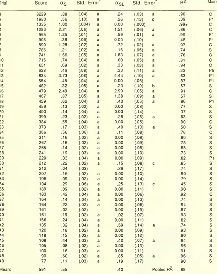
Estimates for

49

trials together with t-statistics are given in table 2.

The

model's

ability to explain the ordering decisions of the subjects is excellent.

R2

varies

between

33%

and

99+%,

with an overall

R^

for the pooled sample of 85%.'* All but

two

ofthe estimates of

a^

are highly significant.

The

supply line adjustment parameter is significant in

22

trials,

and

not significantly different

from

zero in 27.

Of

course, zero is a legitimate value for_{Qsl, and}

the estimate of

a^L

for 23 subjects is zero.

The

estimates of

_a^L

range

from

to 4.4 while the

mean

95%

confidence

band

for the zero estimates is .17, less than

4%

ofthe range ofa^L,

indicating that the

23

zero estimates ofttjL are quite tight.

6.

Simulation

of the estimated decision rules

The

estimation results indicate that the

model

is a

good

representation of the

sub-jects' decision-making.

Sterman

(1988a) analyzes the estimated parameters

and

identifies

D-3976

14

One

ofthese is the tendency for subjects to give insufficient attention to the supply line, as

indicated by the large

number

of small estimates for a^L-

By

ignoring the supply line subjects

continue ordering even after the construction pipeline contains sufficient units to correct any

stock discrepancy.

Such

overordering is a major source ofinstability in the closed loop

sys-tem.

The

present concern, however, is the relationship

between

the estimated parameters

and the regimes of behavior in the model.

Even

though the subjects

do

not

behave

optimally

in disequilibrium,

one

might expect that their decision rules

would

ultimately return the

sys-tem

to a

low

cost equilibrium. Simulation ofthe estimated rules

shows

this is not the case.

The

rightmost

column

ofTable 2 indicates the

mode

of behavior produced

by

simulation of the decision rule with the estimated parameters.

The

parameters estimated for

thirty subjects

_(61%)

are stable.

Most

of these produce

overdamped

behavior of the capital

stock in response to the step input.

Seven

parameter sets produce limit cycles of period 1

and one produces period 5.

The

parameters

which

characterize eleven subjects

(22%)

produce chaos. Inspection of table 2

shows

that the subjects

whose

parameters are stable

performed best in the task while those

whose

parameters produce periodic behavior or chaos

generally

had

the highest costs.

1-way

ANOVA

confirmed the relationship: the costs

achieved by the subjects strongly

depend on

the

mode

produced by

simulation ofthe

estimated decision rule (p<.01

when

the

modes

were coded

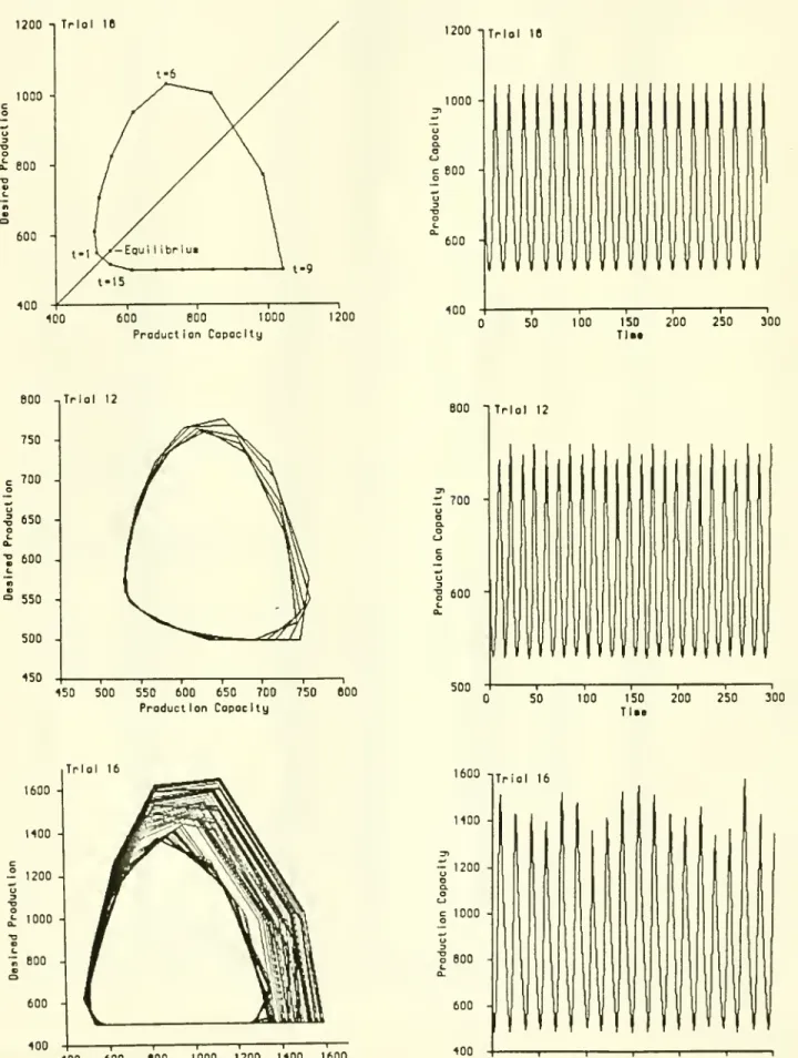
as stable, periodic, or chaotic).

Figure 4

shows

time

domain

and phase portraits for simulations of several sets of

estimated parameters. In all cases the orbits are roughly egg-shaped, with clockwise flow.

To

explicate the dynamics, consider figure 4a,

showing

theperiod 1 limit cycle

produced

by

the parameters of subject 18 (.62, .43;

R^

=

.86). In equilibrium desired production

must

equal

capacity; the locus of such points is given by the 45° line.

Below

the line there is excess

capacity and the system is linear and stable;

above

it there is insufficient capacity and the

system is highly nonlinear and unstable.

Given

the steady input oforders

from

the

goods

sector of

500

units, the equilibrium point for the system as a

whole

lies at (555.55, 555.55).

and

capital sectorgrow. Rising desired production induces additional orders

from

the capital

sector, causing rapid increase in desired production. Capacity, held

down

by

the inability of

the capital sector itself to fill all orders and the consequentrationing ofoutput, lags behind.

As

capital stock grows, however,

new

orders placed by the capital sector slow,

and

the

backlog is shipped at an increasing pace. Desired production peaks at t=6. Capacity

now

grows

rapidly as the capital sector is increasingly able to fill orders.

Between

t=7 and t=8

capacity overtakes desired production,

which

falls rapidly since capacity is

now

large

enough

to deliver the entire supply line in

one

period.

As

desired production

plummets,

capacity

reaches its

peak

and

capital sector orders to fall to zero (t=9). Desired production is then

sustained only by the

exogenous

demand

ofthe

goods

sector (500 units/period).

Deprecia-tion causes capital stock to decline slowly, until at t=15 capital stock has fallen to a level

low

enough

to cause the capital sector to place

new

orders.

However,

these

new

orders cause

desired production torise,

and by

the next period capacity is

once

again insufficient to satisfy

demand,

initiating the next cycle.

The

dynamics

are the

same

for the period multiples and

chaotic solutions, except that the trajectory does not close after

one

orbit.

The

trajectories of chaotic systems are sensitive to initial conditions.

The

routes of

nearby points through phase space diverge exponentially until the initial difference in the

positions balloons out to fill the entire attractor.

The

time average rate ofexponential

divergence of neighboring points is given by the largest

Lyapunov

exponent

L+

[Wolf

et al.

(1985)]

which

may

be defined as

L^=lim|log2|xI

(23)

where

the separation vector x connects neighboring points in phase space.

A

positive

exponent

means

nearby points diverge

and

indicates chaos; a negative

exponent

denotes

convergence

of nearby points.

Because

the

Lyapunov

exponents describe the long-term

D-3976

16

that average, including temporary reversals of sign. Nevertheless, a

rough

estimate of

L+

is

given

by

the slope of

L^(t)t=log2|x| (24)

over long intervals.

To

calculateL^(t)t for each of the estimated decision rules, production

capacity

was

jjerturbed by

one

part in a trillion in the 10,0(X)th period.

The

separation vector

|x|

was measured

in the two-dimensional space defined by production capacity and desired

production. Since desired capacity is the

sum

of the

two

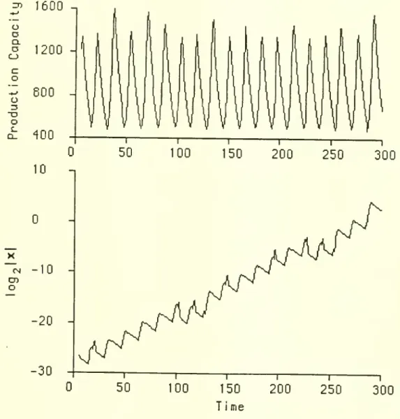
backlogs, this output space reflects

all three state variables in the system. Figure 5

shows

the evolution ofL^(t)t for the

parameters of subject 16 after the perturbation.

The

phase plot for these parameters is

shown

in figure 4.

The

average slope of L^(t)t is clearly positive, indicating the system is

chaotic.

The

magnitude

ofthe

Lyapunov

exponent is approximately .1 bits/period.

The

values of

L^

for the subjects

whose

decision rules are chaotic range

from

about .01 to .1 bits/period,

with an average of about .04 bits/period.

The

magnitudes of the exponents determine the rate at

which

information about the

state of the system, and hence the ability to predict its trajectory, is lost.

The

large

mea-surement errors in

economic

systems

[Morgenstem

(1963)] dictate severe limits

on

pre-dictability in chaotic systems.

Thus

ifthe states ofthe

model

economy

were

known

with the

not unrealistic

measurement

error of about

12%

(3 bits ofprecision), the average

Lyapunov

exponent of .04 implies the uncertainty in the trajectory

would

grow

to fill the entire attractor

afteronly about 75 periods, corresponding in the experimental system to roughly 5 orbits.

Additional precision buys little in additional predictability: cutting

measurement

error by a

factor of

two would

delay the complete loss ofpredictability by less than 2 orbits.

Of

course

these calculations

assume no

external noise, perfect specification of the model, and perfect

estimates ofthe parameters, and thus represent an upper

bound on

the prediction horizon.

7.

Mapping

the

parameter space

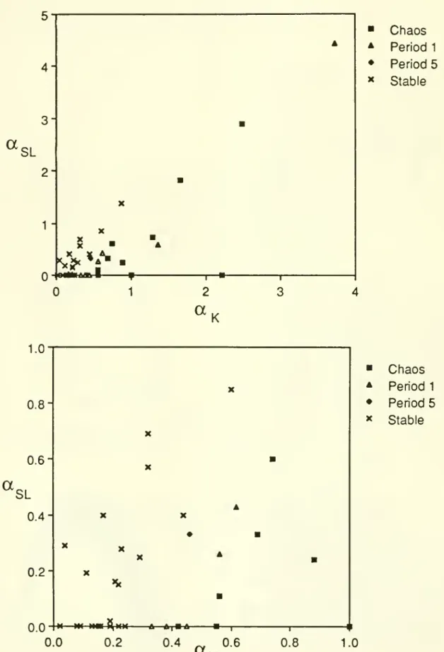
parameters. Figure 6 locates the

modes

of behavior of the estimated decision rules in

parameter space.

The

estimated parameters are clustered in the region

_0<aK<l,

_0<asL^l,

with the

few

outside this region falling approximately along the line cxsL=aK. Consistent with

intuition, the stable decision rules are confined to the region

where

aj^ is small and

_a^L

is

large, while the chaotic decision rules generally involved aggressive stock adjustment

and

weak

supply line adjustment.

More

aggressive attempts to correct the discrepancy

between

the desired

and

actual capital stock are destabilizing:

by

ordering

more

aggressively the

sub-ject induces a larger increase in total

demand,

thus exacerbating disequilibrium and encour-aging still larger orders in future periods. Conversely,

more

aggressive response to the

supply line is stabilizing

by

constraining orders as the supply line fills.

More

formally,

a^

determines the gain of the oscillatory negative feedback loop while

_ajL

controls the

first-order, stabilizing supply line loop.

To

test this hypothesis the estimated parameters

were

regressed

on

the log of the cost function S. Costs provide a rough

measure

ofinstability since

high costs indicate large excursions

from

equilibrium (standard errors in parentheses, trial 1

deleted as an outlier):

ln(S)

=

5.3 -I-

I.TOk-

l.lasL, R2=.43,

F=16.8

(N=48). (25)

(.13) (.33) (.30)

The

results are highly significant and confirm the overall relationship

between

the parameters

and

stability.

But

is the parameter space as

smooth

as these results suggest?

Figure 7

maps

the parameter space for

_0<aK^l

and

0<asL^l

in steps of .005,

representing over 40,CX)0 simulations.^ This region includes

86%

of the estimated parameter

sets, clearly

showing

that the fluctuating steady state solutions, including the chaotic

solutions, lie in the managerially meaningful region of parameter space.

The

resulting

bifurcation structure is surprisingly structured. First, the

boundary

for the bifurcation

from

fixed point to cyclic attractors appears to be a straight line, with stable solutions satisfying

asL

>

2.29aK

- _.706,

R2

= .99946 _{(N=42). (26)}

D-3976

18

Rasmussen,

Mosekilde, and

Sterman

(1985)

show

that the transition

from

local stability to

instability at the equilibriumjx)int involves a

Hopf

bifurcation. In the region

where

capacity

is inadequate (<))<1) the linearized closed-loop system is oscillatory, but for small values of

a^

orlarge values of a^L. the eigenvalues lie inside the unit circle, producing

damped

behavior and a stable fixed-point attractor.

As

the parameters

become

less stable (larger Oj^

or smaller _Csl) the eigenvalues cross the unit circle and the system produces expanding

oscillations.

These

fluctuations are ultimately

bounded by

the nonlinearities, particularly the

nonnegativity constraint

on

orders

and

the flexible utilization ofcapacity in equation (1).

Inside the region of fluctuating steady state solutions, several features are apparent.

Note

first the striations ofperiodic behavior

which

cut across the space at a

somewhat

shallower angle than the stability/instability boundary.

The

bands are thicker near the

transition to stability and thinner

away

from

it. Second, note the several large regions in

which

the periodic solutions are very sparse.

Figure 8 magnifies the region _.55<aK<.65,

_.50<asL^.60

by a factor often in each

direction.

Both

the chaotic regions and the bands of periodic behavior are

now

seen to contain

irregularly distributed islands ofother periodicities. Further magnification (not

shown)

reveals still

more

such islands.

Such

irregularity is characteristic of the fractal boundaries

common

in the bifurcation

maps

of

many

systems.

Simple though the

model

is, it is capable ofgenerating a

wide

array of

complex

behaviors.

The

complexity of the parameter space

shows

that

even

small errors in estimates

of the parameters

may

have large qualitative effects

on

the

mode

of behavior

produced

by the

system. Indeed, the simulations here

do

not exhaust the possibilities. All the simulations

described here involved

no

external forcing (goods sector orders for capital

were

constant).

Larsen, Mosekilde, and Sterman (1988) have

shown

that sinusoidal forcing in

goods

sector

orders (mimicking the effects of the business cycle or othercyclical

modes

in the

economy)

8. Discussion

It is

common

in the social sciences to

assume

that decision-making behavior and thus the

dynamics

of

human

systems are, ifnot optimal, then at least stable.

These

results

show

that formal rules

which

characterize actual managerial decision

making

can produce an

extraordinary range ofdisequilibrium dynamics, including chaos.

Such

complexity suggests strong lessons for modelers of

economic

and social

dynamics.

The

experiment

shows

that the regimes of fluctuating steady-state behavior,

including chaos, lie squarely in the middle ofthe realistic region ofparameter space. In

consequence

modelers can ignore nonlinear

dynamics

only at theirperil.

Models

of

economic

and

social

dynamics

should portray the processes

by which

disequilibrium conditions are

created and dissipated.

They

should not

assume

that the

economy

is in or near equilibrium at

all times nor that adjustment processes are stable.

Models

should be formulated so that they

are robust in extreme conditions, since it is the nonlinearities necessarily introduced

by

robust formulations that crucially determine the

modes

ofthe system [see

Day

(1984)].

At

the

same

time a

number

ofquestions regarding the the generalization of the results

to the real

world

and the practical significance ofchaos

must

be asked.

Chaos

is a

steady-state

phenomenon

which

manifests over very long time frames, but

many

policy-oriented

models

are concerned with transient

dynamics

and nearly all with time horizons

much

shorter

than those used in the analysis of chaotic dynamics.

For

example

the simulations here

were

run for 10,000 periods or more.

Over

such extended time horizons the parameters ofthe

system cannot be considered static but will themselves evolve with learning, evolutionary

pressures,

and

exogenous

changes in the environment.

There

is evidence [Sterman (1988a),

Bakken

(1988)] that subjects begin to learn within just a

few

cycles, modifying the

parameters of their ordering function. It appears that in the present experiment learning

slowly

moves

the subjects

away

from

the chaotic region towards the region of stability.

However,

the existence ofchaos

may

itself

hamper

learning.

Even

though deterministic

D-3976

20

changes in initial conditions or parameters.

Does

such 'randomness' slow the discovery of

cause and effect by agents in the

economy

and thus hinder learning or evolution towards

efficiency? Indeed, does learning alter the parameters ofdecision rules so that systems

evolve towards or

away

from

the chaotic regime?

Some

argue that chaos

may

be adaptive. In a world

whose

'fitness space' contains

many

local optima, a decision rule that produces chaos,

by constantly exploring

new

pathways,

may

help a system evolve faster than a stable,

incremental decision

making

strategy [Prigogine and Sanglier (1987), Allen (1988)].

Chaos

places an upper

bound on

prediction, but is that

bound

a binding constraint in

social systems? Real social systems are

bombarded

by

broadband

noise, and it is well

known

that such

random

shocks severely degrade predictability.

Does

the

magnitude

of

stochastic shocks

swamp

the uncertainty in trajectories caused

by

chaos?

How

does the

existence of chaotic regimes in a

model

influence its response to p)olicies, and the

predictability of thatresponse? Particularly troubling here is the potential for fractal basin

boundaries in both initial condition

and

parameter space. Policy interventions often imply

changes in the parameters ofa decision rule or model.

How

can policy analysis be conducted

if the "policy space" contains fractal basin boundaries? In such systems parameter changes

on

the margin

may

produce unpredictable qualitative changes in behavior, as illustrated by the

fractal distribution of

modes shown

in figures 7-8. Therefore learning and experience

may

not

transfer tocircumstances

which

differonly slightly. Learning often involves a hill-climbing

procedure of incremental

movement

towards a profit-maximizing

peak

in parameter space.

How

well can agents negotiate that space

when

the landscape not only has

many

local

optima but is fractal as well?

The

development

ofprinciples for policy design in such systems

is a major area for future research.

The

practical significance ofchaos and other nonlinear

phenomena

in policy-oriented

models

ofsocial and

economic

behavior remains clouded while

these questions are unanswered.

Some

of these questions

may

be resolved

by

further

9.

Conclusions

The

discovery ofnonlinear

phenomena

such as deterministic chaos in the physical

world naturally motivates the search for similar behavior in the world of

human

behavior. Yet

the social scientist faces difficulties in that search

which do

not plague the physicist, at least

not to the

same

degree. Aggregate data sufficient for strong empirical tests simply

do

not

exist for

many

of the

most

important social systems. Social systems are not easily isolated

from

the environment.

The

huge

temporal

and

spatial scales ofthese systems, vast

number

of actors, costs

and

ethical concerns

make

controlled experiments

on

the systems themselves

difficult at best. Finally, the laws of

human

behavior are not as stable as the laws ofphysics.

Electrons

do

not learn, innovate, collude, or redesign the circuits in

which

they flow.

Laboratory experiments appear to provide a fruitful alternative. Since experiments

on

actual firms

and

national

economies

are infeasible, simulation

models

of these systems

must

be used to explore the decision

making

heuristics of the agents.

Such

experiments create

'microworlds' in

which

the subjects face physical and institutional structures, information, and

incentives

which

mimic

(albeit in a simplified fashion) those ofthe real world. It appears to

be possible to quantify the decision

making

heuristics used

by

agents in such experiments

and

explain theirperformance well. Simulation then provides insight into the

dynamic

properties of the experimental systems.

These

results demonstrate that chaos can be

produced

by the decision

making

processes of real people.

The

experiment presented subjects with a straightforward task in a

common

and

important

economic

setting.

The

subjects' behavior is

modeled

with a high

degree of accuracy

by

a simple decision rule consistent with empirical

knowledge

developed

in psychology

and

long used in

economic

models. Simulation ofthe rules produces chaos for a

significant minority ofsubjects.

Chaos

may

well be a

common

mode

of behaviorin social and

economic

systems, despite the lack ofsufficient information to detect it in aggregate data.

D-3976

22

Notes

1 Journal of

Economic

Theory,

40

(1) 1986, Journal of

Economic

Behaviorand Organization, 8

(3),

September

1987;

System

Dynamics

Review,

4, 1988,

European

Journal ofOperational

Research, 35, 1988. See also

Goodwin,

Kruger, and Vercelli (1984)

and

Prigogine

and

Sanglier (1987).

2. Conservation of output requires

P

=

A

+

AG.

But

A

+

AG

=

_B(t)

+

BG({)

=

(})(B

+

EG)

=

(P/P*)(B +

BG)

= P.

By

Little's law, the average residence time ofitems in a backlog is the

ratio ofthe backlog to the outflow, here given by

A

=

(B +

BG)/(A

+ AG).

By

eq. 4-5, (B +

BG)/(A

+

AG)

=

(B

+

BG)/(B-(t)

+

BG<t))

=

1/<|).

3. Disks suitable for

IBM

PC's and

compatibles, or for the

Apple

Macintosh, are available

from

the author.

4.

Note

that the function 0=f(-) does not contain an estimated regression constant.

Thus

the correspondence of the estimated and actual capital orders, notjust their variation around

mean

values, provides an important

measure

of the model's explanatory power. Since the

residuals e need not satisfy _Zct

=

0, the conventional

R2

is not appropriate.

The

alternative

R2

=

1 - _Xct^ /

ZO,2

is used (Judge et al. 1980). This

R2

can be interpreted as the fraction of

the variation in capital orders around zero explained by the model.

5.

Each

simulation

was

10,000 periods long.

The

first

8000 were

discarded in assessing the

steady state

mode

of behavior. 10 digit accuracy

was

used.

A

simulation

was assumed

to be

References

Allen, P., 1988,

Dynamic

models

of evolving systems.

System

Dynamics

Review,

4.

Bakken,

B., 1988, Learning system structure by exploring

computer

games, presented at the

1988

International

System

Dynamics

Conference,

San

Diego,

CA,

July.

Bamett,

W.

and

P.

Chen,

1988,

The

aggregation theoretic

monetary

aggregates are chaotic

and

have strange attractors: an econometric application of mathematical chaos, in Bamett,

Bemdt, and White

(eds.),

Dynamic

Econometric

Modeling,

Cambridge

University Press,

Cambridge.

Benhabib, J. and R.

Day,

1981, Rational choice and erratic behavior.

Review

of

Economic

Studies, 48, 459-471.

Brehmer,

B., 1987,

Systems

design

and

the psychology of

complex

systems, in

Rasmussen,

J.

and

P.

Zunde

(eds). Empirical Foundations of Information

and

Software Science III,

Plenum,

New

York.

Brock,

W.,

1986, Distinguishing

random

and

deterministic systems: abridged version. Journal

of

Economic

Theory, 40, 168-195.

Camerer,

C,

1981, General conditions for the success of bootstrapping models,

Organizational Behavior and

Human

Performance, 27, 411-422.

Candela, G.,

and

A. Gardini, 1986, Estimation ofa non-linear discrete-time

macro

model.

Journal of

Economic Dynamics

and

control, 10, 249-254.

Chen,

P., 1988, Empirical and theoretical evidence of

economic

chaos.

System

Dynamics

Review,

4, 81-108.

Dana,

R.,

and

P. Malgrange, 1984,

The

dynamics

ofa discrete version ofa

growth

cycle

model, in Ancot, J. (ed.). Analysing the Structure of

Econometric Models,

Martinus

Nijhoff,

The

Hague.

Dawes,

R., 1982,

The

robust beauty ofimproper linear

models

in decision making, in

D-3976

24

Cambridge

University Press,

Cambridge.

Day,

R., 1982, Irregular

Growth

Cycles,

American

Economic

Review,

72, 406-414.

Day,

R., 1984, Disequilibrium

Economic

Dynamics:

A

Post-Schumpeterian Contribution,

Journal of

Economic

Behaviorand Organization, 5, 57-76.

Day,

R., and

W.

Shafer, 1985, Keynesian chaos. Journal of

Macroeconomics,

7, 277-295.

Einhom,

H., D. Kleinmuntz, and B. Kleinmuntz, 1979, Linear regression

and

process-tracing

models

ofjudgment. Psychological

Review,

86, 465-485.

Forrester, J. 1961, Industrial

Dynamics,

MIT

Press,

Cambridge.

Goodwin,

R., 1951,

The

nonlinear accelerator and the persistence of business cycles,

Econometrica, 19, 1-17.

Goodwin,

R.,

M.

Kruger,

and

A. Vercelli, 1984, Nonlinear

models

offluctuating growth,

Springer Verlag, Berlin.

Grandmont,

J.-M., 1985,

On

endogenous

competitive business cycles, Econometrica, 53,

995-1046.

Grassberger, P.,

and

I. Procaccia, 1983,

Measuring

the strangeness of strange attractors,

Physica,

9D,

189-208.

Grether, D.,

and

C. Plott, 1979,

Economic

theory of choice and the preferencereversal

phenomenon, American

Economic

Review, 69, 623-638.

Hogarth, R., 1987,

Judgment

and Choice,

2nd

ed., John Wiley, Chichester.

Hogarth, R., and

M.

Reder, 1987, Rational Choice:

The

contrast

between economics

and

psychology. University of

Chicago

Press, Chicago.

Holt,

C,

F. Modigliani, J.

Muth,

H. Simon, 1960, PlanningProduction, Inventories, and

Work

Force, Prentice-Hall,

Englewood

Cliffs, N.J.

Judge et al., 1980,

The

Theory

andPractice ofEconometrics,Wiley,

New

York.

Larsen, E., E. Mosekilde, and J. Sterman, 1988, Entrainment

between

the

economic

long

wave

and other

macroeconomic

cycles, presented at the

IIASA

Conference

on

Low,

G., 1980,

The

multiplier-accelerator

model

of business cycles interpreted

from

a system

dynamics

perspective, in J. Randers (ed.), Elements of the

System

Dynamics

Method,

MTT

Press,

Cambridge.

MacKinnon,

A., and A. Wearing, 1985, Systems analysis and

dynamic

decision making, Acta

Psychologica, 58, 159-172.

Metzler, L., 1941,

The

nature

and

stability ofinventory cycles.

Review

of

Economic

Statistics,

23, 113-129.

Morgenstem,

O., 1963,

On

the

Accuracy

of

Economic

Observations,

2nd

ed., Princeton

University Press, Princeton.

Plott, C. R., 1986, Laboratory experiments in economics:

The

implications of posted price

institutions. Science,

232

(9

May),

732-738.

Prigogine, L,

and

M.

Sanglier, 1987,

Laws

ofnature

and

human

conduct.

Task

Force of

Research Information

and

Study on Science, Brussels.

Ramsey,

J.,

and

H.-J.

Yuan,

1987, Bias and error bars in dimension calculations and their

evaluation in

some

simple models,

New

York

University.

Ramsey,

J., C. Sayers,

and

P.

Rothman,

1988,

The

statistical properties ofdimension

calculations using small data sets:

some

economic

applications,

RR88-10,

New

York

University

Department

of

Economics.

Rasmussen

and

Mosekilde, 1988, Bifurcations

and

chaos in a generic

management

model,

European

Journal ofOperational Research, 35, 80-88.

Rasmussen,

S., E.

Mosekilde

and J. Sterman, 1985, Bifurcations

and

chaotic behavior in a

simple

model

ofthe

economic

long wave,

System

Dynamics

Review,

1, 92-1 10.

Samuelson, P. A., 1939, Interactions

between

the multiplier analysis

and

the principle of

acceleration.

The Review

of

Economic

Statistics, 21, 75-78.

Senge, P., 1980,

A

system

dynamics

approach to investment function formulation and testing,

Socio-Economic

Planning Sciences, 14, 269-280.

D-3976

26

Slovic, P.

and

S. Lichtenstein, 1983, Preference reversals: a broaderperspective,

American

Economic

Review,

73, 596-605.

Smith, V. L., 1982,

Microeconomic

systems as an experimental science,

American

Economic

Review, 72

, 923-955.

Smith, V. L., 1986, Experimental

methods

in the political

economy

ofexchange, Science, 234,

(10 October), 167-173.

Sterman, J. D., 1985,

A

behavioral

model

ofthe

economic

long wave.Journal of

Economic

Behavior and Organization, 6, 17-53.

Sterman, J. D., 1987, Testing behavioral simulation

models

by direct experiment.

Management

Science, 33 , 1572-1592.

Sterman,J. D., 1988a, Misperceptions offeedback in

dynamic

decision making, Organizational

Behavior and

Human

Decision Processes, forthcoming.

Sterman, J. D., 1988b,Eteterministic chaos in

models

of

human

behavior: Methodological

issues

and

experimental results.

System

Dynamics

Review,

4, 148-178.

Sterman, 1988c,

Modeling

managerial behavior: Misperceptions offeedback in a

dynamic

decision

making

experiment,

Management

Science, forthcoming.

Sterman, J. D.

and

D. L.

Meadows,

1985,

STRATEGEM-2:

a

microcomputer

simulation

game

ofthe Kondratiev Cycle, Simulation

and

Games,

16, 174-202.

Stutzer, M., 1980, Chaotic

dynamics

andbifurcation in a

macro

model.Journal of

Economic

Dynamics

and

Control, 2, 353-376.

Takens, P., 1985, Distinguishing deterministic and

random

systems, in Borenblatt,

G,

G.

looss, and D. Joseph (eds.). Nonlinear

Dynamics

and

Turbulence, Pitman, Boston. Tversky, A. and D.

Kahneman,

1974,

Judgment

under uncertainty: heuristics

and

biases.

Science. 185 (27 September), 1124-1131.

Wolf, A., J. Swift, H. Swinney, and J. Vastano, 1985, Determining

Lyapunov

exponents

from

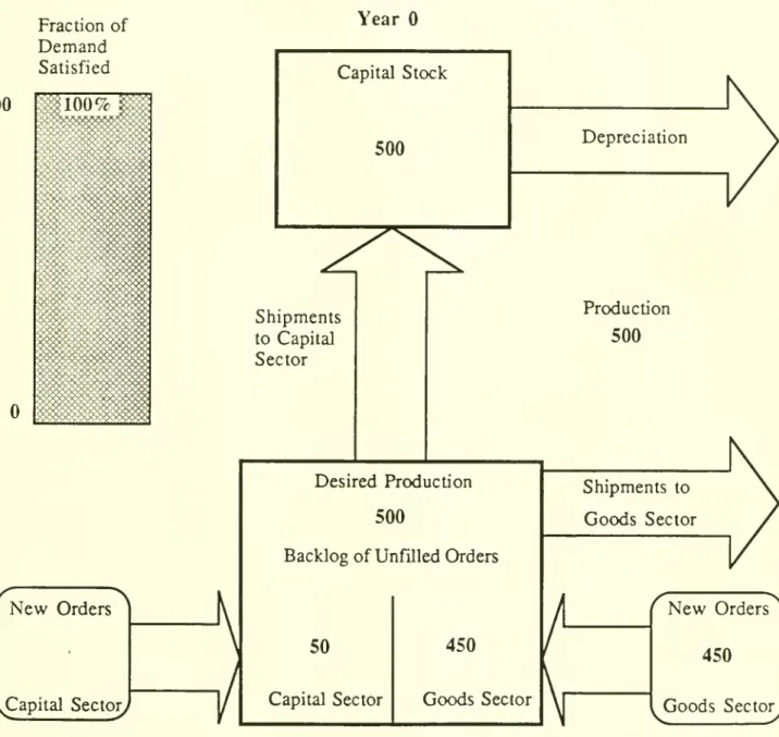
a

Figure 1.

Computer

screen

showing

experimental

economy,

initial configuration.

The

subject is about to enter

new

orders for capital sector.

Fraction of

Demand

Satisfied

Year

100

New

Orders ^Capital Sector; Capital Stock

500

Shipments

to Capital Sector Desired Production

500

Backlog ofUnfilled Orders

50

Capital Sector

450

Goods

Sector Depreciation Production

500

Shipments

to

Goods

Sector

V

New

Orders

450

Goods

Sector,

D-3976

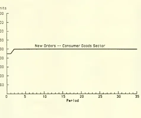
28

Figure 2.

Exogenous

orders ofthe

goods

sector.

Each

trial begins in _{equilibrium. In period 2}

there is an

unannounced

step increase in

_new

_{orders placed}

_by

_the

consumer goods

sector

from 450

to

500

units.

Compare

_{against subjects' behavior}

shown

in figure 3. Units 900 r 600 700 -600 -500 -100 -300 -200 100

\y

New Orders

—

ConsumerGoods Sector

' ' ' I L_I_J L.

10 15 20

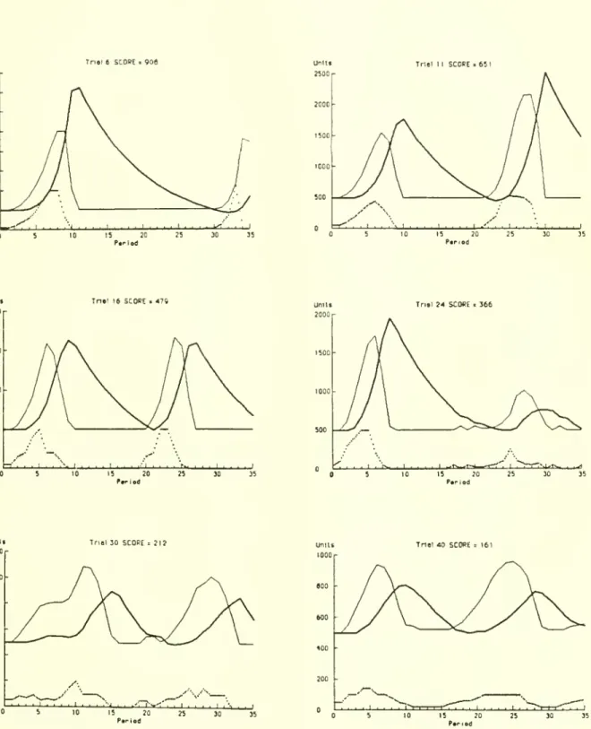
Period

Figure 3. Typical experimental results. N.B.: vertical scales differ.

Desired Producrion Production Capacity Subject'sOrdersforCapital

Tnei6 SCORE•90S _TntI

1I SCOCE.651 IS 20 Parlod Tn»l 16SCORE•*T> Tnil24 SCOREt366 Unit! 1200

D-3976

30

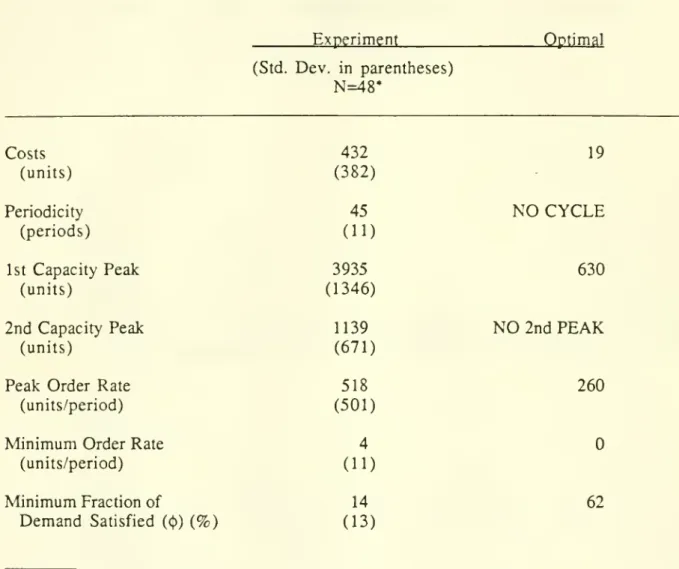
Table 1.

Summary

of experimental results.

Experiment

Optimal

(Std.

Dev.

in parentheses)

N=48*

Costs

Table 2. Estimated parameters and

mode

of behavior of simulated decision rules

D-3976

32

Figure 4. Simulation ofestimated decision rules.

Note

similarity to the experimental results

(figure 3).

-D-3976

33

Figure 5. Evolution oflog2|x|, the distance

between

two

neighboring trajectories, for

simulation with parameters of subject 16 (2.49, 2.90) after perturbation ofcapacity by factor of

vl2

10 in period 10,000.

The

largest

Lyapunov

exponent, given approximately by the average

slope, is positive, indicating that the

two

trajectories diverge exponentially

and

the system is

chaotic. ="

₁₆₀₀

-, CJ

-10

-I en

o

-20

--30

50

300

00

—

150

Ti

me

200

250

300

D-3976

₃₄

Figure 6.

Modes

of behavior

produced

by simulation of the estimated parameters.

Lower

graph magnifies area

bounded

by

0<aK<l,

0<asL^l.

Chaos

*

Period 1

Period 5

« Stable

Chaos

* _Period 1 Period

5

X _Stable