HAL Id: hal-00776740
https://hal.archives-ouvertes.fr/hal-00776740
Submitted on 28 Apr 2021HAL is a multi-disciplinary open access
archive for the deposit and dissemination of sci-entific research documents, whether they are pub-lished or not. The documents may come from teaching and research institutions in France or abroad, or from public or private research centers.
L’archive ouverte pluridisciplinaire HAL, est destinée au dépôt et à la diffusion de documents scientifiques de niveau recherche, publiés ou non, émanant des établissements d’enseignement et de recherche français ou étrangers, des laboratoires publics ou privés.
Distributed under a Creative Commons Attribution| 4.0 International License
Thermo-Mechanical Modeling of a Glacier-Permafrost
System in Spitsbergen, Implications for Subglacial
Hydrology
R. Roux, C. Grenier, C. Marlin, E. Delangle, Albane Saintenoy, J.-M. Friedt,
M. Griselin
To cite this version:
R. Roux, C. Grenier, C. Marlin, E. Delangle, Albane Saintenoy, et al.. Thermo-Mechanical Modeling of a Glacier-Permafrost System in Spitsbergen, Implications for Subglacial Hydrology. EGU General Assembly 2012, Apr 2012, Vienne, Austria. �hal-00776740�
1
Thermo-Mechanical Modeling of a Glacier-Permafrost System in Spitsbergen,
Implications for Subglacial Hydrology
Roux Nicolas, Grenier Christophe
Laboratoire des Sciences du Climat et de l’Environnement, UMR 8212 CNRS-CEA-UVSQ, Orme des merisiers, 91191 Gif-sur-Yvette Cedex, France
Marlin Christelle, Delangle Emerick, Saintenoy Albane
IDES, UMR 8148 CNRS – Université Paris Sud, 91405 Orsay Cedex, France Friedt Jean-Michel
FEMTO-ST, UMR 6174 CNRS, Université de Franche-Comte, France Griselin Madeleine
THEMA, UMR 6049 CNRS, Université de Franche-Comte, France
Abstract
Within the framework of climate change, a small polar glacierized watershed was monitored. Field surveys show winter discharges causing large icings. A 2D modeling approach along the main axis of the system is developed to study the evolution of the glacier-bed system. Two codes are chained (one for the glacier and one for the porous media). Results confirm that the glacier is polythermal with a cold based terminus. Its rapid retreat (20 m.a-1) should lead to a cold glacier within decades to a century. Simulations show that permafrost development precedes glacier retreat (thin glacier tongue with -5°C mean annual air temperatures measured at Ny Alesund) while in the mountainous part with a somewhat stable glacier position, permafrost could develop over longer times and extend deep. The unfrozen porous medium extension below the glacier will progressively reduce resulting in the disappearance of winter discharges most probably within this century.
Keywords: Permafrost; Numerical modeling; Glacier-Permafrost interaction; Glacial Hydrology
Introduction
Spitsbergen has been intensively studied in the framework of climate change. Studied are glacier evolution, water fluxes, and terrestrial sediment inputs to the sea.
Several glaciers are located along the Broggerhalvoya peninsula (Northwestern Spitsbergen) with similar features. For instance, Midre Lovenbreen was extensively studied. A French mission has been studying the neighbor Austre Lovenbreen with a special focus on the hydrology of the catchment (liquid and solid). This site is optimal for such studies because the glacier zone is separated from the sea outlet by a calcareous layer through which flow has carved a canyon making flux measurement easy and conservative. The glacier system has been extensively studied as well (radar study, Saintenoy et al., 2011; Friedt et al., 2010, 2011). According to the current knowledge, AL is expected to be a polythermal glacier with a cold based terminus. Glacial hydrology is classically complex involving various flow paths within glacier, sub glacial and porous medium (e.g. Fountain and Walder, 1998; Flowers and Clarke, 2002). One especially interesting feature concerns evidences of winter flows. They appear as icings (Griselin, 1982, 1985) covering the glacier forefield. The total volume was estimated by (Griselin, 1985) and some of the flux was recently monitored. Considering the waters geochemistry, this winter flow may be related with the discharge of an underground storage volume probably refilled from upper parts of the
Fig. 1: On the upper right corner, the study area (black oval) in Northwestern Spitsbergen, the Broggerhalvoya. Study glacier with surface and bed topography (respectively solid and dotted lines). Bed and surface contour intervals are 50m and 20m respectively. Past extension from 1962 DEM is shown as well (outermost solid line).
Our objective here is to study the validity of such an assessment by means of glacier and permafrost modeling. The extension of permafrost is indeed a key feature controlling the extension of this probable subglacial or porous medium reservoir. Due to the highly transitory properties of the coupled system, its evolution is considered, involving some future perspectives.
The modeling approach involves a glacier model and a heat transfer simulation code for porous media. Both models are simply chained: glacier evolution is simulated and basal temperature evolution is used as forcing signal to the porous medium heat transfer model. The uncovered parts of the profile are imposed air temperatures. This approach is similar to (Boulton and Hartikainen, 2004, in the framework of nuclear waste storage studies and considering ice sheets, see Chan et al., 2005). Similarly again, the model is a 2D cut through the system.
The key idea is that a sufficiently thick and active glacier should maintain ice temperatures at the pressure melting point at its base. Indeed, the glacier insulates the ground from the atmosphere, and geothermal flux will accumulate at the glacier base, resulting in an elevation of basal ice temperature. As observed by the French surveys, the glacier has been retreating over the last decades and its thinning is leading to the freezing of its base due to the reduction of activity and of curtain effect (annual mean air temperatures are well below zero).
In the sequel, we present the Thermo-Mechanical glacier model, the permafrost model, and the simulations.
Glacier modeling
Glacier and Bedrock geometry
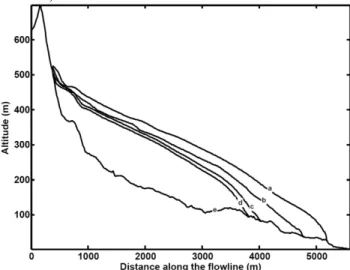
Since 2006, both glacier surface and bedrock have been mapped with Differential GPS for the surface and Ground Penetrating Radar for the ice thickness. The Digital Elevation Model corresponding to 2009 including glacier surface and bedrock is used. The horizontal resolution is 10 m (see Figure 1 for the contour plot). DEMs for the 1995 and 1962 surfaces also exists (Friedt et al., in prep.). We extract from each DEM a South to North flowline profile as an input for the 2D glacier model (Fig. 2). Glacier retreats rapidly, roughly 20 m.a-1 over the last 50 years. The first profile (a) in Figure 2 corresponds to an initial reconstruction of glacier extension at the hypothesized beginning of the recession (1925) as explained below.
Mass balance and temperature profiles
Extensive mass balance measurements are available for three years between 2007 and 2010. From those data we inferred a linear relation linking mass balance to the
altitude, which we will apply to any surface geometry. The constant relation over the years is justified by the fact that the glacier net mass balance in this area has been fairly constant, though negative over the past few decades (Hagen et al. 1990, 2003).
Temperature measurements at the glacier surface give a pretty well constrained and constant altitudinal temperature gradient (5.7 °C.km-1). We thus apply this gradient to the measured temperature at Ny Alesund (43 m.a.s.l) to have the surface temperature profile. We use as a reference the mean annual air temperature over the last seventy years (-5°C, data from the Norsk Meteorological Institute).
Fig. 2: Flowline profiles. “a” is the 1925 estimate of the glacier surface. “b”, “c” and “d” are from the 1962, 1995 and 2009 DEM respectively. “e” is the bedrock.
The model
We used the thermo-mechanically coupled model developed by Sam Pimentel during its stay at Simon Fraser University, Vancouver, Canada. Only the glacier dynamics part has been published in Pimentel et al. (2010), where full description of the model can be found. In the mechanical part, the momentum and mass conservation equations with the constitutive flow law, which depends on stress and temperature, are resolved in a Picard iteration loop. Surface boundary is stress free whereas sliding can be applied at the glacier base. Modifications are made in the original thermal part, resulting in an energy conservation equation reduced to the simplest, which is vertical heat conduction and volumetric heat source due to the internal deformation of ice.
Simulations
The current thermal state of the glacier is certainly not in balance with the current climate, especially now in its transitory state due to its long time of retreat. The high heat storage capacity of ice should make inertial effects important. We thus need, in order to best reproduce today thermal field, to have a genetic approach of the glacier that we see today. We inferred a former flowline profile from the ground extent from the “Little Ice Age” (LIA) that we think is marked by the moraine (Fig. 2).
Similarly to Zwinger & Moore (2009), we let the glacier with the “LIA” geometry equilibrate between the surface temperature and the geothermal heat flux applied at its base. A constant flow law parameter for ice is used. We then use this thermal state as an initial state for the prognostic simulations. The glacier evolution is then resolved thermo-dynamically over 200 years.
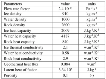
Table 1. Constants and model parameters used for both glacier and porous media numerical models.
Parameters value units
Flow rate factor 2.4 10-24 Pa-3.s-1
Ice density 910 kg.m-3
Water density 1000 kg.m-3
Rock density 2600 kg.m-3
Ice heat capacity 2009 J.kg-1.K-1
Water heat capacity 4187 J.kg-1.K-1
Rock heat capacity 840 J.kg-1.K-1
Ice thermal conductivity 2.1 w.m-1.K-1
Water heat conductivity 0.58 w.m-1.K-1
Rock heat conductivity 2.9 w.m-1.K-1
Geothermal heat flux 0.084 w.m-2
Latent heat of fusion 3.34 105 J.kg-1
Porosity 0.1 (-)
Permafrost modeling
The model
A coupled Thermo-Hydraulic code was developed recently (Régnier et al., 2010) within the Cast3M finite element and finite volume code (www-cast3m.cea.fr). The purely thermal model used here simulates transient heat transfers with conduction and phase change. The equation (e.g. similar to McKenzie et al., 2007) is non linear. The conductive properties depend on the thermal state of the porous medium and the liquid water saturation curve is a linear function of temperature providing a temperature range of 1.5°C for phase change (from full liquid water saturation to full ice saturation). The non linearity is dealt with by a Picard convergence loop.
Simulations
The simulated domain is 2D, complementing the glacier mesh. Its upper part corresponds to the ground surface including the glacier bed and lateral extensions (to the mountain summit and to the sea). The modeled zone spreads 200 m into the ground. The upper boundary condition is imposed temperatures obtained from glacier simulations at its bed. For the part of the domain not corresponding to the glacier extension, air temperatures are imposed. Lower boundary is imposed geothermal flux. Sides are constrained to no heat flux. Tab. 1 provides ground thermal properties used for the simulations.
Results
Glacier evolution and basal temperature
Glacier surface evolution over 200 years is plotted in Figure 3. The modeled 1962 and 2009 glacier surface is in very good agreement with the data. We can then date the initial surface profile by looking at the time needed to model the surface closest to data. This gives for both 1962 and 2009 data an initial profile of 1925 with a 5 years uncertainty (Fig. 3). Modeled surface for 1962 and for 2009 are pretty close to the data (Fig. 3). Figure 3.b shows the basal temperature modeled at the initial state and in 1962 and 2009 with the transient method. Figure 3.c is the same as Figure3.b but, for each geometry, the glacier is in equilibrium with climate. It shows how important it is to go back in time as far as we can to model the correct current thermal state. If the glacier was to be in equilibrium with today’s climate, its base would be entirely cold.
Figure 4 shows today modeled thermal state. The temperate part of the glacier is very small, and we should be close to an entirely cold based glacier.
Fig. 3: (a) 1962 and 2009 modeled surface (solid) compared with the data (dotted line). Smallest glacier extent corresponds to the 2125 modeled surface. (a) & (b) Modeled basal temperature at the 1925 initial state (solid), 1962 (dotted) and 2009 (dashed).
Fig. 4: (a) 1962 and 2009 modeled surface (solid) compared with the data (dotted line). Smallest glacier extent corresponds to the 2125 modeled surface. (a) & (b) Modeled basal temperature at the 1925 initial state (solid), 1962 (dotted) and 2009 (dashed).
Permafrost extension
Simulation starts from unfrozen conditions. It is more precisely the result of a steady state calculation with geothermal flux at the base and an upper limit with 0°C. This is probably accurate below the glacier and reasonably close to the shoreline, the impact of the sea being in maintaining annual temperatures closer to 4°C. The conditions up the mountain are hard to estimate considering the literature. For instance, (Humlum, 2005) provides estimates of permafrost depths around 500 m in the mountains of Spitsbergen. The present case corresponds to steep summits with very close glaciers which probably limited the permafrost development as compared with this estimation. For the sake of simplicity, we start here from no permafrost and study permafrost development in the system. The whole simulation corresponds to 200 years, from 1925 to 2125. It spreads over the present state with the additional idea of getting a prospective view to permafrost development over larger time scales.
Fig. 5: Permafrost development as a function of glacier retreat: ice thickness profiles are positives and plotted with a 50 years interval; depth of the -0.5°C isotherm in the porous medium are negatives. The dashed line corresponds to the stand by year 2009.
Figure 5 shows the impact of rapid glacier retreat (20 m.a-1 during last 50 years) in its lower end while the temperature
variations close to the summit are reduced. The temperature at the base of the glacier (Figure 3.b) forces surface heat transfer model in the porous medium. The top of Figure 5 provides glacier thicknesses through time. The maximum extension is represented as dotted line, corresponding to the 1925 initial reconstruction from Figure 2. The dashed line corresponds to present state while the other curves (from 1 to 4) correspond to the states after a 50 time interval. The lower part of Figure 5 provides the position of the -0.5°C isotherm in the porous medium. Results show that the two sides of the domain behave differently. The lower part (glacier tongue) sees rapid lateral evolution permafrost: the glacier retreats and the permafrost progression precedes the glacier retreat due to the reduced thickness of the mouth of the glacier allowing the penetration of the cold wave. For the upper part of the domain on the other hand, the position is maintained but the cold wave penetrates deeper due to exposure time and progressive small thinning of the glacier thickness. Air temperatures are about 3 °C lower than down the glacier due to altitudinal effects. This provides a more intense permafrost development. We expect that this thickness would be higher with a longer exposure time.
Discussion
We have a system that is way out of equilibrium with today’s climate. But be that as it may, the reconstructed glacier geometry for 1925 gave us a pretty good look back at the inertial effects for the glacier at least. Ideally the same should be done for the underground media, but there is no such feature as the moraine to enable us to guess a former extension of permafrost. In fact, we could let the permafrost develop for thousands of years with some realistic upper temperature profile for the mountain peak. This would only give us an idea of “a maximum” depth of high mountain permafrost. By doing so, we obtained permafrost depths of the order of 400 m, over 5000 years, which is in good agreement with former estimations (Humlum, 2005). It is more difficult to “guess” in the same way a maximum depth for costal permafrost. It is probable that our calculation for today extent isn’t so far from reality. Indeed, only a really small area should have been exposed to air temperature for a long time, since the glacier, before landing on the ground, was most certainly calving to the sea.
Our model thus provides a simplified but coherent view of the glacier-underground system at least from a qualitative point of view. Some quantitative features are probably reasonably estimated. For instance, permafrost extension under the glacier is at least 500 m long beneath the glacier tongue. Its retreat reduces the unfrozen bed zone roughly at the same speed (20 m.a-1). The upper part of the profile presents no evolution of glacier cover but the temperature signal penetrates into the massif and permafrost propagates at depth and partly below the glacier. The reduction of unfrozen bed extension is slower but its quantitative velocity is subject to uncertainties due
to difficulties in estimating the initial temperature field conditions in the mountains. According with the model, and considered scenarios, the time required to obtain complete freezing of the porous medium below the glacier ranges between 20 years and a century. Thus, winter flows will probably reduce in the following decades. A hydrogeological model should take these extensions into account, considering that permafrost zones are no flow zones. The water recharge to the bed is probably achieved in summer along the bergschrund while winter discharge, limited by permafrost at the base of the tongue, requires sub glacier outflow channels. This is coherent with field observations and interpretations by (Griselin, 1985).
Conclusion
We studied here the quantitative evolution of a glacier-porous medium system with a view to the implications on the unfrozen subglacial porous medium layer, probably responsible for winter flows.
Our results are in agreement with radar observations in the glacier and provide a base to explain winter flows. The glacier system is in a rather rapid evolution, forced by climate evolution, which seems to be accelerating recently. It nevertheless follows with some inertia such that a glacier in thermal balance with present conditions would be cold.
Permafrost development is forced by glacier retreat on the lower end. For the upper mountainous zone, the cold wave propagates locally as the glacier becomes thinner. So, the glacier is in transition to becoming cold and time scales are probably of the order of some decades to a century before underground flow vanishes.
Improvements of the approach are currently expected along the following lines. Several scenarios should be considered to address the uncertainties of the system. Among them, the initial permafrost extensions are subject to debate. The underground heat transfer model could be made more complex and treat snow cover, presence of winter icing. The actual nature of the interface between glacier and bed is highly uncertain including the type of heat transfer between glacier and bed. Especially, would underground flow delay permafrost development under the glacier? The retroaction of ground temperatures on the glacier evolution is an open topic.
In the future we will focus on the unfrozen porous medium extension at the base of the glacier as deducted from permafrost development. The simulation of winter discharge with a hydrogeological model will allow us to assess the credibility of the hypotheses and study the range of variations of associated properties.
References
Boulton, G., Hartikainen, J., 2004. Thermo-Hydro-Mechanical Impacts of Coupling Between Glaciers and Permafrost, In: Ove Stephanson, Editor(s), Elsevier Geo-Engineering Book Series, Elsevier, 2004, Volume 2, Pages 293-298.
Chan, T., Christiansson, R., Boulton, G.S., Ericsson, L.O., Hartikainen, J., Jensen, M.R., Mas Ivars, D., Stanchell, F.W., Vistrand, P., Wallroth, T., 2005. DECOVALEX III BMT3/BENCHPAR WP4: The thermo-hydro-mechanical responses to a glacial cycle and their potential implications for deep geological disposal of nuclear fuel waste in a fractured crystalline rock mass. International Journal of Rock Mechanics and Mining Sciences, 42, 5-6, 805-827. Flowers, G. E., and G. K. C. Clarke, 2002. A
multicomponent coupled model of glacier hydrology, 1, Theory and synthetic examples, J. Geophys. Res., 107(B11), 2287.
Fountain, A.G. and Walder, J.S., 1998. Water flow through temperate glaciers. Reviews of Geophysics 36: 299-328.
Friedt, J.-M., Tolle F., Bernard E., Griselin M., Laffly D., Marlin C., 2011. Assessing Digital Elevation Models relevance to evaluate glacier mass balance: application to the Austre Lovenbreen (Spitsbergen, 79oN).
Friedt, J.-M., Laffly, D., Saintenoy, A., Bernard, E., Griselin, M., Marlin, C., 2010. Evaluating the Austre Lovénbreen (Svalbard) glacier ice volume, area and its bedrock topography using Ground Penetrating Radar and differential GPS measurements. 11th International Circumpolar Remote Sensing Symposium. 20-24 September 2010, Cambridge UK Griselin, M., 1985. Les marges glacées du Loven Est,
Spitsberg : un milieu original lié aux écoulements sous-glaciaires. Revue de Géologie Alpine, tome LXXIII, Num. 4, 389-419.
Griselin, M., 1982. Les modalités de l’écoulement liquide et solide sur les marges polaires : exemple de bassin Loven Est, côte nord ouest du Spitsberg. Thèse de troisième cycle, Volume III des travaux du Laboratoire de Géographie Physique de Nancy II. Hagen J.O., Liestol O., 1990. Long-term glacier
mass-balance investigations in Svalbard, 1950-88. Annals of Glaciology 14: 102-106.
Hagen J.O., Kohler J., Melvold K., Winther J.G., 2003. Glaciers in Svalbard: mass balance, runoff and freshwater flux. Polar Research 22: 145-159.
Hansen, S., 2003. From surge-type to non-surge-type glacier behaviour: midre Lovenbreen, Svalbard. Annals of Glaciology 36: 97-102.
Humlum, O., 2005. Holocene permafrost aggradation in Svalbard. In Cryospheric Systems: Glacier and Permafrost. Geological Society, London, Special publication, 242, 119-130.
McKenzie J. M., Voss, C.I., Siegel, D.I., 2007. Groundwater flow with energy transport and water–ice phase change: Numerical simulations, benchmarks, and application to freezing in peat bogs. Advances in Water Resources, 30, 4, 966-983.
Pimentel, S., Flowers, G.E., Schoof, C.G., 2011. A hydrologically coupled higher-order flow-band model of ice dynamics with a Coulomb friction sliding law. J. Geophys. Res 115.
Régnier, D., Grenier, C., Davy, P., Benabderrahmane, H., 2010. A coupled Thermo-Hydro model to study permafrost. Proc. EUCOP III in Longyearbyen, Svalbard.
Saintenoy, A., Friedt, J.-M., Tolle, F., Bernard, E., Laffly, D., Marlin, C., Griselin, M., High density coverage investigation of the Austre LovenBreen (Svalbard) using Ground Penetrating Radar. 6th International Workshop on Advanced Ground Penetrating Radar 2011, Aachen, Germany, 22. – 24.06.2011
Zwinger T. and Moore J.C., 2009. Diagnostic and prognostic simulations with a full Stokes model accounting for
superimposed ice of Midtre Lovénbreen, Svalbard. The Cryosphere 3: 217-229