HAL Id: hal-00618696
https://hal.archives-ouvertes.fr/hal-00618696
Submitted on 2 Sep 2011
HAL is a multi-disciplinary open access
archive for the deposit and dissemination of
sci-entific research documents, whether they are
pub-lished or not. The documents may come from
teaching and research institutions in France or
abroad, or from public or private research centers.
L’archive ouverte pluridisciplinaire HAL, est
destinée au dépôt et à la diffusion de documents
scientifiques de niveau recherche, publiés ou non,
émanant des établissements d’enseignement et de
recherche français ou étrangers, des laboratoires
publics ou privés.
Fast model of space-variant blurring and its application
to deconvolution in astronomy
Loïc Denis, Éric Thiébaut, Ferréol Soulez
To cite this version:
Loïc Denis, Éric Thiébaut, Ferréol Soulez. Fast model of space-variant blurring and its application to
deconvolution in astronomy. ICIP 2011, Sep 2011, Bruxelles, France. pp.2873-2876. �hal-00618696�
FAST MODEL OF SPACE-VARIANT BLURRING
AND ITS APPLICATION TO DECONVOLUTION IN ASTRONOMY
L. Denis, E. Thi´ebaut
Observatoire de Lyon, CRAL CNRS UMR 5574,
UCBL, ENS de Lyon, Universit´e de Lyon,
France
F. Soulez
Centre Commun de Quantim´etrie,
Universit´e Lyon 1, Universit´e de Lyon,
France
ABSTRACT
Image deblurring is essential to high resolution imaging and is therefore widely used in astronomy, microscopy or com-putational photography. While shift-invariant blur is modeled by convolution and leads to fast FFT-based algorithms, shift-variant blurring requires models both accurate and fast. When the point spread function (PSF) varies smoothly across the field, these two opposite objectives can be reached by inter-polating from a grid of PSF samples.
Several models for smoothly varying PSF co-exist in the literature. We advocate that one of them is both physically-grounded and fast. Moreover, we show that the approximation can be largely improved by tuning the PSF samples and inter-polation weights with respect to a given continuous model. This improvement comes without increasing the computa-tional cost of the blurring operator.
We illustrate the developed blurring model on a deconvo-lution application in astronomy. Regularized reconstruction with our model leads to large improvements over existing re-sults.
Index Terms— deconvolution, shift-variant PSF
1. INTRODUCTION
Image deconvolution is widely used to enhance the resolu-tion, signal-to-noise ratio and contrast of blurred images. In many cases, blur is space-variant and thus can no longer be modeled by a convolution. Accurate modeling of the point spread function (PSF) is essential for restoration. Depend-ing on whether PSF variations across the field are smooth or discontinuous, PSF are either interpolated, or the field is seg-mented into regions inside which PSF are invariant. In the former case, effort is put in finding a good tradeoff between approximation quality and speed. The most challenging as-pect of the latter case is the segmentation step.
In astronomy, blurring due to atmospheric turbulence varies in the field of view. Even after adaptive optics cor-rection, the PSF is shift-variant since the correction quality
This work has been supported by project MiTiV funded by the French National Research Agency (ANR DEFI 09-EMER-008-01).
decreases away from the guiding star[1]. Optical aberrations and obstructions also lead to space-variant degradations[2]. In 3D microscopy, the 3-D PSF varies with the depth from the coverslip[3]. In all these applications, PSF vary smoothly. Except for very compact PSF, the storage and applica-tion of a different PSF for each pixel[4] is not computa-tionally tractable for iterative deblurring methods. It has then been proposed[5] to decompose the image into patches where blur can be considered approximatively invariant (iso-planatic regions). After deconvolution of each patch, the reconstructed regions must be tied together which leads to border artifacts[6, 3, 7]. It is therefore preferable to model smooth blur variations and then, to deblur the whole image.
Smooth PSF variations can be decomposed on a subspace of PSF[8, 9]. The cost of this modeling increases linearly with the number of basis PSF used. It has been noticed independently by several authors that PSF variations could be modeled by interpolation and yet lead to a fast blurring model[10, 11, 12]. Two formulations have been proposed, equivalent in terms of computational complexity but leading to different PSF models. We discuss in section 2.1 these two approximations and their implications in terms of PSF model-ing. We show that one of them is superior both in approxima-tion quality and modeling properties. In secapproxima-tion 2.2, we fur-ther improve PSF approximation error by tuning the PSF sam-ples and interpolation weights for a target PSF model. The space-variant blurring model is then applied to deconvolution of Hubble Space Telescope (HST) simulated data. We show improved reconstructions compared to the results reported on the same dataset in [10].
2. APPROXIMATION OF SMOOTHLY VARYING PSF During the formation of an imageg, the original (crisp) distri-butionf undergoes distortions due to atmosphere turbulence, object/camera relative motion, the instrument (limited aper-ture, optical aberrations). These degradations are typically modeled by a linear transform:
g(r) = Z
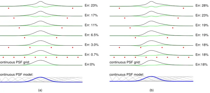
Fig. 1. Comparison of (a)H and (b) H†for PSF approximation (blue: target PSF, red: PSF sample locations, green:
approxi-mation error).
whereh denotes the point spread function (PSF). When the PSF does only depend on the difference r− s, equation (1) is a convolution and the system is said isoplanatic.
2.1. PSF interpolation
Smoothly varying PSF can be approximated by interpolating PSF at locations siwith interpolation kernelϕint:
h(r, s) ≈X
ihi(r − s) ϕint(s − si), (2)
withhi(u) ≡ h(si+ u, si) the PSF for a source located at
si. The image formation model is then approximated by: g(r) ≈X
i
Z
hi(r − s) ϕi(s) f (s) ds ≡ [H◦f ](r), (3)
whereϕi(s) = ϕint(s − si) and H denotes the linear
oper-ator of our approximate model. This operoper-ator and its adjoint (which is needed for image reconstruction) expand as:
H =X iHi◦Wi and H ♯=X iWi◦H ♯ i, (4)
withWi a scaling operator corresponding to the pointwise
multiplication byϕi,Hi andH♯i a convolution and a
corre-lation by theith sampled PSF. In words, Eq. (3) expresses the degraded image as the sum of convolutions between PSF samples and weighted versions of the crisp image.
An alternative model has been proposed by [10] who in-terpolate the result of convolving the original image by the PSF samples. The corresponding operator writes:
H†=X
iWi◦Hi. (5)
[12] uses formulationH and [11] give both. Note that H†
is similar to the adjointH♯ of our operator (using
convolu-tions instead of correlaconvolu-tions); hence the computational burden are the same for both. Though closely related, the operators H and H† are however different in their ability to correctly
approximate the shift-variant PSF. Figure 1 gives a mono-dimensional illustration of the difference between the two. We consider a system with Gaussian PSF whose standard de-viation increases linearly with the position from left to right. Several of these Gaussian PSF are drawn in light gray on last row of the figure. The target PSF at the center of the field is drawn in thick blue stroke. This PSF is approximated using PSF samples at locations depicted by red dots: coarse sam-pling at the top row, and refined samsam-pling at the next rows until continuous sampling for the last but one. A linear in-terpolation kernel is used. The formulation ofH is used for sub-figure 1(a), whileH†is used for sub-figure 1(b).
Approx-imation errors are drawn in green, and the relative norm of the error is given at the right of each curve. Several properties of the approximations are noticeable: (i) PSF interpolation (H) preserves PSF symmetry, while interpolation of convolution results (H†) does not; (ii) when the PSF supports are small
compared to the distance between two PSF sample locations, the two approximations are comparable; (iii)H achieves ex-act interpolation (i.e., PSF approximation error tends to zero when the PSF grid is ever more refined) whileH† does not;
(iv) PSF positivity and normalization are preserved by linear interpolation (which is not the case withH†, even when a
lin-ear interpolation kernel is used). Based on the difference be-tween the two models, we recommend the use of formulation H rather than H†for smoothly varying blurs.
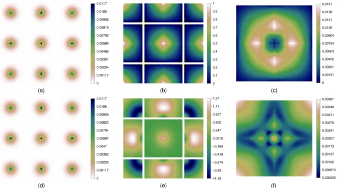
Fig. 2. PSF approximation: (a)-(c) using bilinear interpolation; (d)-(f) generalized interpolation with optimal PSF and weights; (a), (d): PSF grid; (b), (e): interpolation weights on each of the 9 patches; (c), (f): rms error with respect to target PSF.
As noted in [10, 11, 12], operatorsH and H† can be
ef-ficiently computed using fast Fourier transforms (FFT). Each term of the sum in Eq. (4) is a convolution of a PSF (sizeH2)
with a patch whose sizeB2corresponds to the support of the
interpolation kernel (for a grid ofK2 PSF samples, an N2
image, and linear interpolation,B = 2N/K). Each discrete convolution requiresO[(B + H)2log(B + H)] operations,
thus the whole operator requiresO[K2(B +H)2log(B +H)]
operations. If the PSF supportH is much smaller than the support of the interpolation kernel, the computational cost is O[4N2log N ] operations, i.e., 4 times the cost of a single
convolution of the whole image. Table 1 reports the computa-tion time of our parallel implementacomputa-tion of operatorH (based on FFTW and Linux pthread libraries, running on an Intel Xeon 3.3GHz with 6 cores). When the PSF support is large compared to the support of the interpolation kernel, most of the computational effort is spent computing the boundaries of each patch and the complexity raises as illustrated by the last rows of table 1.
2.2. Improvement of the approximation
There are several options to improve the approximation er-ror: (i) refine the interpolation grid (costly when the PSF sup-port is large); (ii) increase the interpolation order (huge cost since the support of the interpolation kernel is proportional to the interpolation order); (iii) use generalized interpolation, i.e., refine interpolation weightsϕi (with constant
interpola-tion support) and PSF sampleshito fit a target PSF.
nb of threads 1 2 4 6
PSF grid time in ms (relative to a convolution) 5 × 5 71 (3.7) 37 (1.9) 19 (1) 14 (0.7) (a) 10 × 10 46 (2.4) 22 (1.2) 11 (0.6) 8 (0.4) 20 × 20 60 (3.2) 30 (1.6) 15 (0.8) 11 (0.6) 5 × 5 182 (4.2) 97 (2.3) 57 (1.3) 47 (1.1) (b) 10 × 10 636 (15) 325 (7.6) 170 (4) 117 (2.7) 20 × 20 1680 (39) 850 (20) 435 (10) 293 (6.8)
Table 1. Average time to compute operatorH: (a) 5122pixels
image, with31 × 31 pixels PSF; (b) 10002pixels image, with
101 × 101 pixels PSF (Intel Xeon Processor with 6 cores).
Option (iii) is the most interesting since it improves the approximation without increasing the computational cost of H. We achieve this by minimizing the quadratic difference:
ǫ2= 1 N2 Z Z h h(r, s) −X ihi(r − s) ϕi(s) i2 dr ds (6)
with respect to the PSF {hi}K
2
i=1 and the weights {ϕi}K
2
i=1.
Starting with the PSF samples, we alternately solve for the best weights, and then for the best PSF samples. Using this algorithm, the approximation can be largely improved (the rms errorǫ is divided by 4, which is better than when using a 6 × 6 grid with linear interpolation), as illustrated by figure 2.
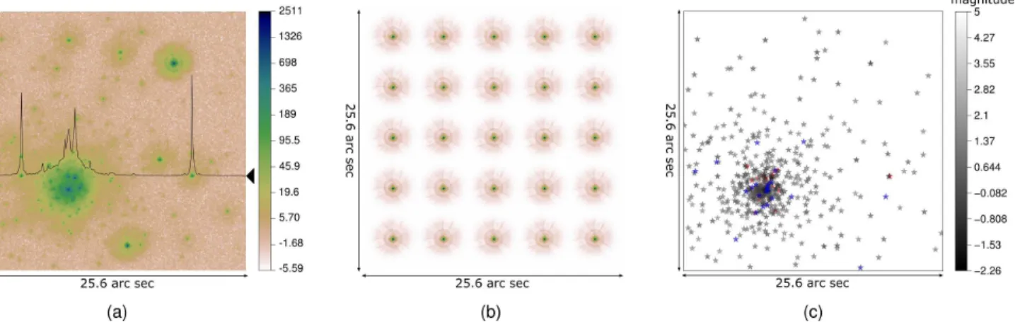
Fig. 3. Deconvolution with shift-variant PSF: (a) simulation of an observation of a star field with Hubble’s Wide Field Camera before corrective optics; (b) provided5 × 5 grid of PSF; (c) recovered stars after deconvolution with sparsity prior, gray: good detection, blue: non-detected star (4.9%), red: false-detection (7.2%)
2.3. Application to deconvolution in astronomy
We used the same dataset as in [10] to illustrate the applica-tion of our model on a realistic astronomical case. Contrary to [10] who used truncated preconditioned conjugate gradi-ents, we performed regularized inversion with anℓ1
sparsity-inducing prior and a positivity constraint (minimization done with FISTA algorithm [13]). Figure 3 presents the obtained results: rms error is 3.6% when using5 × 5 PSF grid, 6.2% when using the mean PSF, to be compared with the 16% error reported in [10]. The use of a regularization largely improves the reconstruction. The spatially-variant PSF model further improves the results.
3. CONCLUSION
We have shown that PSF interpolation is physically more jus-tified and leads to a better approximation of space-variant PSF. The computational cost remains modest (4× that of a single convolution). We proposed to further improve the model accuracy while keeping the same computational cost. We applied our model to a realistic astronomical case. Our next step will be to extend our approach to blind or myopic deconvolution, in wide-field adaptive optics and microscopic imaging.
4. REFERENCES
[1] G. Cresci, R.I. Davies et al., “Accounting for the anisopla-natic point spread function in deep wide-field adaptive optics images,” A& A, vol. 438, pp. 757–767, 2005.
[2] J. Anderson and I.R. King, “Toward High-Precision Astrome-try with WFPC2. I. Deriving an Accurate Point-Spread Func-tion,” Pub. Astr. Soc. Pac., vol. 112, pp. 1360–1382, 2000. [3] C.Preza and J.-A. Conchello, “Depth-variant
maximum-likelihood restoration for three-dimensional fluorescence
mi-croscopy.,” J Opt Soc Am A, vol. 21, no. 9, pp. 1593–1601, 2004.
[4] M.K. Ozkan, A.M. Tekalp, and M.I. Sezan, “POCS-based restoration of space-varying blurred images,” IEEE Trans. Im-age Process., vol. 3, no. 4, pp. 450–454, 1994.
[5] H. Trussell and B. Hunt, “Image restoration of space-variant blurs by sectioned methods,” IEEE Trans. Acoust., Speech, Signal Process., vol. 26, no. 6, pp. 608–609, 1978.
[6] M. Aubailly, M. Roggemann et al., “Approach for reconstruct-ing anisoplanatic adaptive optics images.,” Appl Opt, vol. 46, no. 24, pp. 6055–6063, 2007.
[7] A.F. Boden, D.C. Redding et al., “Massively parallel spatially variant maximum-likelihood restoration of Hubble Space Tele-scope imagery,” J Opt Soc Am A, vol. 13, no. 7, pp. 1537–1545, 1996.
[8] R. Flicker and F. J Rigaut, “Anisoplanatic deconvolution of adaptive optics images.,” J Opt Soc Am A, vol. 22, no. 3, pp. 504–513, Mar 2005.
[9] M. Arigovindan, J. Shaevitz et al., “A parallel product-convolution approach for representing the depth varying point spread functions in 3D widefield microscopy based on prin-cipal component analysis.,” Opt Express, vol. 18, no. 7, pp. 6461–6476, 2010.
[10] J.G. Nagy and D.P. O’Leary, “Restoring Images Degraded by Spatially Variant Blur,” SIAM J. Sci. Comp., vol. 19, pp. 1063, 1998.
[11] E. Gilad and J. Hardenberg, “A fast algorithm for convolution integrals with space and time variant kernels,” J. Comp. Phys., vol. 216, no. 1, pp. 326–336, 2006.
[12] M. Hirsch, S. Sra, B. Scholkopf, and S. Harmeling, “Efficient filter flow for space-variant multiframe blind deconvolution,” in IEEE Comp. Vis. Pattern Recogn., 2010, pp. 607–614. [13] A. Beck and M. Teboulle, “A fast iterative
shrinkage-thresholding algorithm for linear inverse problems,” SIAM J. Imaging Sci., vol. 2, no. 1, pp. 183–202, 2009.