HAL Id: inserm-00336116
https://www.hal.inserm.fr/inserm-00336116
Submitted on 17 Sep 2009
HAL is a multi-disciplinary open access
archive for the deposit and dissemination of sci-entific research documents, whether they are pub-lished or not. The documents may come from teaching and research institutions in France or
L’archive ouverte pluridisciplinaire HAL, est destinée au dépôt et à la diffusion de documents scientifiques de niveau recherche, publiés ou non, émanant des établissements d’enseignement et de recherche français ou étrangers, des laboratoires
Model-based analysis of myocardial strain data acquired
by tissue Doppler imaging.
Virginie Le Rolle, Alfredo Hernandez, Pierre-Yves Richard, Erwan Donal, Guy
Carrault
To cite this version:
Virginie Le Rolle, Alfredo Hernandez, Pierre-Yves Richard, Erwan Donal, Guy Carrault. Model-based analysis of myocardial strain data acquired by tissue Doppler imaging.. Artificial Intelligence in Medicine, Elsevier, 2008, 44 (3), pp.201-219. �10.1016/j.artmed.2008.06.001�. �inserm-00336116�
1 2
Model-Based Analysis of Myocardial Strain Data acquired by Tissue
3
Doppler Imaging
4 5
Virginie Le Rolle1 2, Alfredo I. Hernández1 2, Pierre-Yves Richard 4, Erwan Donal1 2 3 and Guy Carrault1 2 6
7
1 INSERM U642, Rennes, F-35000, France
8
2 Université de Rennes 1, LTSI, Rennes, F-35000, France.
9
3 CHU Rennes, Department of Cardiology, Rennes, F-35000, France
10
4 Supelec-IETR, Rennes, France.
11 12 email: 13 [email protected] 14 tel: 15 (33) 2 23 23 55 85 16 fax: 17 (33) 2 23 23 69 17 18 address : 19
LTSI, Campus de Beaulieu, 20
Université de Rennes 1, 21
263 Avenue du Général Leclerc 22
CS 74205 - 35042 Rennes Cedex, France. 23
24
Summary
:25
Objective: Tissue Doppler Imaging (TDI) is commonly used to evaluate regional ventricular contraction
26
properties through the analysis of myocardial strain. During the clinical examination, a set of strain signals is 27
acquired concurrently at different locations. However, the joint interpretation of these signals remains 28
difficult. This paper proposes a model-based approach in order to assist the clinician in making an analysis of 29
myocardial strain. 30
Methods and material: The proposed method couples a model of the left ventricle, which takes into account
31
cardiac electrical, mechanical and hydraulic activities with an adapted identification algorithm, in order to 32
obtain patient-specific model representations. The proposed model presents a tissue-level resolution, adapted 33
to TDI strain analysis. The method is applied in order to reproduce TDI strain signals acquired from two 34
healthy subjects and a patient presenting with Dilated Cardiomyopathy (DCM). 35
Results: The comparison between simulated and experimental strains for the three subjects reflects a
36
satisfying adaptation of the model on different strain morphologies. The mean error between real and 37
synthesized signals is equal to 2.34% and 2.09%, for the two healthy subjects and 1.30% for the patient 38
suffering from DCM. Identified parameters show significant electrical conduction and mechanical activation 39
delays for the pathologic case and have shown to be useful for the localization of the failing myocardial 40
segments, which are situated on the anterior and lateral walls of the ventricular base. 41
Conclusion: The present study shows the feasibility of a model-based method for the analysis of TDI strain
42
signals. The identification of delayed segments in the pathologic case produces encouraging results and may 43
represent a way to better utilize the information included in strain signals and to improve the therapy 44
assistance. 45
Index Terms— Biomedical Systems modeling, Biomedical Model Simulation, Model-Based
46
Interpretation, Echocardiography
47 48
48
1. Introduction
49
In the daily clinical practice, Doppler Echocardiography has become a fundamental method in evaluating the 50
cardiac function. This non-invasive technique is particularly useful for the analysis of blood flow and cardiac 51
anatomy, facilitating the diagnosis of cardiovascular pathologies. Tissue Doppler Imaging (TDI) is a more 52
recent tool that can be useful in assessing regional myocardial deformations through the estimation of 53
regional myocardial strain [1, 2] and strain rate [3]. Myocardial strain analysis has shown to be useful, for 54
example, in differentiating healthy and ischemic myocardium [4, 5]. More details on TDI acquisition and 55
analysis are presented in appendix A. 56
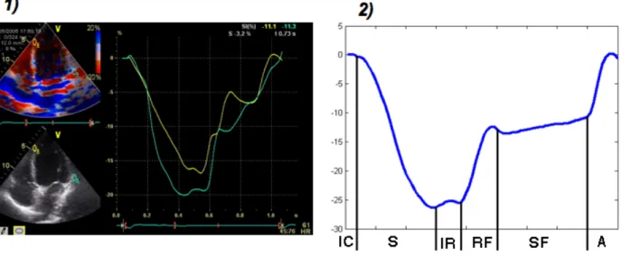
A typical experimental strain signal is shown in figure 1. Tissue extensions correspond with positive strains 57
while tissue compressions result in negative strains. This signal reflects the different phases occurring during 58
the cardiac cycle (figure 1): i) the isovolumic contraction phase; ii) the systole; iii) the isovolumic relaxation; 59
iv) the diastole, which can be divided into three periods: the first one corresponding to a rapid filling phase
60
due to an aspiration of blood inside the ventricle, a slower filling period and the late diastolic filling phase, 61
corresponding to the atrial systole. 62
Although TDI presents some disadvantages such as a dependence on the ultrasound beam orientation [1], 63
that affects the reproducibility, and the presence of noise [2], it has been successfully validated by the 64
comparison with other imaging methods, like MRI or sonomicrometry [2, 6]. The main advantages of TDI 65
are related to the possibility of obtaining real-time measurements and the relative low cost of this technique. 66
67
Figure 1: 1) Tissue Doppler Imaging applied to a four-cavity echocardiographic acquisition. 2) A typical experimental strain of a segment can 68
be divided in several phases: isovolumic contraction (IC), ejection (S), isovolumic relaxation (IR), rapid filling (RF), slow filling period (SF) 69
and atrial systole (A) 70
Several indicators can be derived from strain estimations, such as maximum systolic velocity or ventricular 71
filling period [4, 7]. Although the use of such indicators has already shown interesting results in identifying 72
some cardiovascular pathologies, the whole information contained in the strain signal is not yet fully utilized. 73
The analysis of the morphology of a set of strain signals, acquired concurrently at different regions of the 74
myocardium, is a very difficult task. This is partly due to the multidimensionality of the problem and the fact 75
that the different processes which lead to ventricular contraction (mechano-hydraulic interactions, electrical 76
activation and propagation, etc.) have to be jointly considered for an appropriate interpretation. 77
In this paper we propose a model-based approach to assist the clinician on the analysis of myocardial strain 78
signals. A brief presentation of current approaches for modeling the electromechanical activity of the heart is 79
proposed in section 2. Section 3 describes the proposed ventricular model and the parameter identification 80
method. Finally, in section 4, the results of patient-specific identifications and the analysis of strain 81
morphologies are presented and discussed. 82
2. Current electromechanical models of the cardiac function
83
A variety of mathematical models of the ventricular function have been proposed in other studies. The 84
simplest models are based on a time-varying elastance [8, 9]. These overall, lumped-parameter models give 85
realistic simulations of cardiac pressure and volume and require low computational resources. However, as 86
the whole left ventricle (LV) is represented as a single element, it is not possible to analyze the regional 87
ventricular function. Other approaches have been proposed in order to represent explicitly, at many different 88
levels of detail, the cardiac electrical activity, the excitation-contraction coupling, the mechanical activity 89
and the mechano-hydraulic coupling. The main modeling techniques applied to represent these activities are 90
briefly recalled in the following paragraph. 91
2.1. Electrical Activity
92
Models of the cardiac electrical activity, defined at the cell level, can be classified into three categories: 93
• Biophysical continuous models, composed of detailed descriptions of the cardiac action-potential, 94
based on the Hudking-Huxley formulation [10], and presenting different levels of detail on the ionic 95
currents included [11-13]. 96
• Phenomenological continuous models, which reproduce qualitatively the electrical activation 97
without describing the different ion channels. They present less computational requirements and 98
result in simplified representations of the model’s electrical activity (often based on the FitzHugh-99
Nagumo model [14]). 100
• Simplified discrete models, they are often based on cellular automata, representing the different 101
electrical states of a myocyte’s action potential [15]. 102
Coupling of cell-level continuous models in order to represent a patch of myocardial tissue, or more complex 103
geometries such as the whole LV, can be performed by using the monodomain or bidomain approaches [16, 104
17]. Cellular automata are typically coupled by means of a discrete flag transmitted to all neighbors during 105
the depolarization of each element [18]. Another approach to represent the propagation of the cardiac 106
electrical activity is limited to modeling the evolution of the depolarization wavefront through the cardiac 107
2.2. Mechanical Activity
109
The ventricular mechanical activity is usually described as a function of its active and passive properties. 110
Active properties are the consequence of the shortening and lengthening of sarcomeres, which are the 111
elementary mechanical contractile elements of myocytes. This mechanical activity is under the influence of 112
an electrical activity, since the variation of calcium concentration during the action potential allows the 113
development of force. Passive properties are mainly related to fiber structure and orientation, collagen 114
properties and metabolic conditions (such as hypoxia or ischemia). 115
116
Models of the active properties include: 117
• Huxley-type models, which represent changes of conformation on sarcomeres as a function of cross-118
bridge position [20] and intracellular calcium concentration [21]. 119
• Hill's models, which use one of the forms of the original Hill’s force-length relation [22-24] or the 120
modified Hill equation, which is a sigmoid function relating calcium concentration and active 121
tension. 122
• The HMT model, proposed by Hunter–McCulloch–ter Keurs [25], which includes a rather detailed 123
description of protein kinetics associated with myofilament length modifications. 124
• Phenomenological approaches, which are based on time-varying analytical activation functions that 125
reach their minimum during diastole and their maximum during systole. A number of such analytical 126
functions have been proposed, with different forms and parameters, such as in [26, 27]. 127
128
Passive myocardial properties are mainly described through specific mechanical constitutive laws. Most of 129
these mechanical laws are hyperelastic, incompressible and anisotropic [28-30]. The majority of them have 130
been determined using uniaxial [31] or biaxial tension tests [30]. An empiric law based on the description of 131
sarcomere dynamics has been proposed by [22]. 132
133
The simulation of these models are often based on finite-element methods (FEM) [32-35]. Although this 134
kind of formulation allows a rather detailed description of the myocardium dynamics, it requires significant 135
computational resources. Another complementary approach for modeling the myocardium deformation is 136
based on a mass-spring system [36] activated by a model of the electrical activity through a simplified 137
electro-mechanical coupling. 138
2.3. Fluid-structure interaction and boundary conditions
139
The simulation of a realistic cardiac cycle requires the representation of the interaction between the 140
myocardium and the blood inside the heart’s chambers and in the systemic and pulmonary circulations. 141
Several approaches to this have been proposed: 142
• Fluid-structure interaction models integrate simultaneous descriptions of the fluid inside the cavity, 143
by means of a Navier-Stokes formulation [37, 38] and the myocardial wall motion, based on the 144
description of a constitutive law, as presented in the previous section. 145
• Rule-based definition of boundary conditions: In most FEM models of the LV, boundary conditions 146
are imposed by the intra-ventricular pressure, by means of a set of rules defining different levels of 147
pressure for each phase of the cardiac cycle. The ejection and filling phase can be deduced from a 148
simplified model of the circulation [32, 34], while a penalty pressure is applied during the 149
isovolumetric phases, in order to keep the volume constant [39]. An alternative method has been 150
proposed in a recent paper, combining a lumped parameter model of the circulation with an FEM 151
model of the ventricles, based on the estimation of an equivalent overall ventricular elastance for 152
each time-step [40]. These approaches imply the uniformity of blood pressure inside the cavity. 153
However, Courtois et al have shown the importance of regional pressure gradients in the LV, 154
especially during diastole [41]. 155
2.4. Model-based analysis of strain signals
156
Complete models of ventricular activity are developed from a combination of the several different 157
approaches previously described and some of these models have been applied to the analysis of myocardial 158
strain. Nickerson et al [42] proposed a 3D model of cardiac electromechanics and used the fiber extension 159
ratio to study the role of electrical heterogeneity in the cardiac function. The model includes a precise 160
description of ventricular contraction, but requires around three weeks of simulation time on a parallel 161
computer in order to reproduce one beat. Kerckhoffs et al [27] have proposed a 3D finite element model of 162
cardiac mechanics used to compare synthesized ventricular strain signals generated by a normal and a 163
synchronous electrical activation sequence. The model simulations show unphysiological contraction 164
patterns when a physiological electrical activation is applied. Results illustrate the difficulty of using such a 165
model in a concrete clinical application and the necessity of representing heterogeneous electromechanical 166
couplings. The same model has been used by Ubbink et al [43] to study circumferential and circumferential-167
radial shear strain. Simulated strains are compared to Magnetic Resonance Tagging (MRT) data. The model-168
based approach helps in determining the influence of fiber angle on regional contraction. However, as the 169
model includes simplified descriptions of its hydraulic activity, the whole morphology of ventricular strain 170
cannot be analyzed, especially during the rapid filling phases. 171
172 173
As previously stated, the main objective of this study is to propose a personalized model-based approach in 174
order to assist the clinicians in the interpretation of myocardial strain signals measured with Tissue Doppler 175
echocardiography. The models described in the previous paragraphs are difficult to apply in this case, as they 176
are characterized by a significant number of parameters, require significant computational resources and, 177
consequentially, their ability to be identified is more complex. Previous studies [44] have shown the benefit 178
of combining a minimal cardiovascular model and an identification algorithm for real-time patient specific 179
necessary for this particular study, a new model has thus been developed, with the following specific 181
properties: 182
• The model resolution has been adapted to the problem, keeping a similar abstraction level as the 183
experts for the analysis of strain signals. 184
• The model is based on a functional integration of interacting physiological processes, by taking into 185
account: i) the electro-mechanical coupling, ii) the interactions between the myocardial wall and the 186
blood inside the cavity and iii) a simplified representation of the systemic circulation. This allows the 187
representation of the main cardiac properties required to tackle the problem under study, like the 188
Frank-Starling law and the influence of preload and afterload. 189
190
The next section presents a detailed description of the proposed model and the identification algorithm which 191
is applied in order to obtain patient-specific model parameters. 192
3. Materials and methods
193
3.1. Model description
194
3.1.1. General presentation of the proposed model
195
In order to simulate the strain measured for each myocardial region, the proposed LV model has been 196
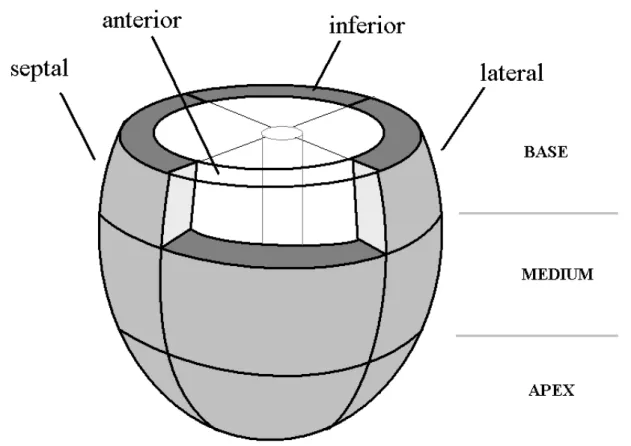
divided into twelve segments, composed of three layers at the basal, equatorial and apical level [45]. Each 197
layer is separated into 4 components: septal, lateral, anterior and inferior wall (figure 2). Each wall segment 198
interacts with the blood inside the corresponding intra-ventricular cavity (which is itself segmented in a 199
consistent manner). It should be noticed that such a 12-wall segmentation does not correspond to the 200
standard myocardial segmentation defined in [46]. However, this segmentation has already been used in 201
different studies (such as in [45]) and remains significant from a clinical standpoint. 202
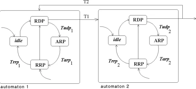
The LV has been approximated by a truncated ellipsoid as it has already produced encouraging results in 203
other studies, for the analysis of the electrical propagation during contraction [19, 47] or ventricular torsion 204
[48]. The choice concerning the modeling formalism for each cardiac activity are summarized here: 205
• Electrical activity: A cellular automata network has been chosen to describe the electrical activation 206
sequence for the 12 segments. This formalism presents low computational costs, while describing the 207
basic properties of the cardiac electrical activity. 208
• Mechanical activity: The myocardium has been supposed to be hyperelastic, incompressible and 209
transverse isotropic. The twist motion of the ventricle has been neglected, as it cannot be measured 210
with tissue Doppler echocardiography. As circumferential and longitudinal strains are less sensitive 211
to cardiac fiber angle [43], only a mean fiber angle is taken into account. 212
• Hydraulic activity: A lumped parameter model is used to describe the hydraulic activity of the intra-213
ventricular cavity and the influence of preload and afterload. This representation is adapted to 214
reproduce major cardiac properties like the Frank-Starling law and the representation of regional 215
pressure gradient that has been observed in the LV [41]. 216
The proposed model can be seen as an improvement of elastance models, by representing a set of sub-pumps 217
interconnected in the hydraulic domain and commanded by a coordinated electrical activity. Each pump 218
represents a macroscopic, tissue-level segment of the LV wall. 219
220
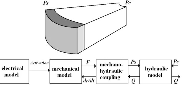
Figure 2: Ventricular model segmentation. The model is composed of 12 segments, corresponding to the septal, lateral, anterior and inferior 221
components for three different layers (basal, equatorial and apical). This graphical representation will be used in figure 12. 222
223
3.1.2. Electrical activation model
224
The ventricle has been represented by twelve cellular automata to describe the electrical propagation during 225
contraction. Each automaton is defined by four electrical states [49, 50] (figure 3): i) rapid depolarization 226
period (RDP), ii) absolute refractory period (ARP), iii) relative refractory period (RRP) and iv) a waiting 227
period (idle). The transitions between states happen spontaneously at the end of the duration of each phase 228
or due to an external activation, during the idle or RRP states. After the RDP period, each automaton 229
transmits a stimulus to its neighboring segments. Each automaton is fully connected (antegrade and 230
retrograde connections) to its three or four neighbors. An external excitation first stimulates the mid-septum 231
segment and is then propagated to the other segments in function of each automaton’s parameter values. 232
233
Figure 3: States and coupling conditions for cellular automata models. Each automaton is characterized by four electrical states: i) rapid 234
depolarization period (RDP), ii) absolute refractory period (ARP), iii) relative refractory period (RRP) and iv) a waiting period (idle). 235
236
Electrical activation has been described as an anisotropic propagation [51], as the conduction delay is about 237
three times longer in the horizontal direction than in the vertical direction. The coupling between two cellular 238
automata is defined by the period
€
T1 for the antegrade link and the period
€
T2 for the retrograde link (see
239
figure 3). For a vertical coupling, these periods are defined as
€
T1= Trdp1 and
€
T2 = Trdp2. For a horizontal 240
coupling, they are equal to
€ T1= 3.Trdp1 and € T2= 3.Trdp2. 241
3.1.3. Mechanical–hydraulic model
242The radial force developed by each segment is computed by integrating the radial stress on the wall surface. 243
Myocardial stress is usually expressed as the sum of active and passive stresses. 244
€
Fr=
∫
σr.dS=∫
(σra+σrp).dS (1)245
The active stress can be expressed using the relation: 246
€
σa = Ta.(FN ).(FN )
T (2)
247
where F is the deformation gradient tensor, N stands for a unitary vector in the fiber direction and
€
Ta is the 248
active tension. As in other studies [26, 27],
€
Ta is approached by means of a trigonometric function. In this 249
case, the
€
Ta function is inspired from the studies of Hunter et al [25] and is defined as: 250 € Ta= Tref [Ca2+] i n [Ca2+] i n + Ca50 n [1 +β(λ− 1)] (3) 251
where Tref is the value of the tension at λ = 1,
€
Ca50 the calcium concentration at 50% of the isometric tension,
252
n is the Hill coefficient determining the shape of the curve and β is the myofilament “cooperativity”. The
253
parameters values and functions for
€
Ca50and n are taken from [25].
€
[Ca2+]
i is the intracellular calcium 254
concentration, which represents the mechanical activation level, and is defined in this model as: 255
€
[Ca2+]i=
0 tes< 0
K sin(π .tes/Tmax) 0 ≤ tes ≤ Tmax
0 tes> Tmax (4) 256
Where tes is the time elapsed since the end of the RDP for each segment s, Tmax the activation duration and K
257
the maximum level of calcium concentration. The deformation gradient tensor F can be defined by 258
characterizing the myocardial motion in spherical coordinates. Supposing that a material particle in the 259
undeformed state (
€
R,Θ,Ψ) goes to (
€
r,θ,ϕ) in the deformed state, a radial deformation can be described by: 260 € r = r(R); € θ = Θ ; € ϕ = Ψ (5) 261
These relations define a square diagonal matrix F that includes the strains
€
λr, λθ and λϕin the three principal
262
directions. It can easily be shown that the deformations in these directions are expressed as:
€
λr= ∂r ∂R and
263
€
λθ =λϕ = r R, the latter common value being usually denoted by λ. Additionally, the myocardium is
264
supposed to be incompressible, which is a classical assumption for the cardiac muscle, and the following 265
additional property holds:
€
det(F) = 1. So a simple relation between
€ λr and € λ can be found: € λr = 1 λ 2. 266
The passive stress is due to myocardium organization (fibers, collagen…) and can be expressed using the 267 equation: 268 € σp= − pI + 2F ∂W ∂C F T (6) 269
where W is the strain energy function, p stands for the hydrostatic pressure, I is the identity matrix and C is 270
the Cauchy-Green tensor computed from F through
€
C = FTF. The energy function used in this paper is the
271
one defined by Humphrey et al. [28], which is a polynomial energy function. The polynomial form facilitates 272
the implementation and has shown its efficiency in many studies [48, 52]: 273 € W = c1(α− 1) 2 − c2(α− 1) 3 + c3(I1− 3) + c4(I1− 3)(α− 1) + c5(I1− 3) 2 (7) 274 Where € I1 and €
α = I4 stand for the invariants of the deformation gradient tensor. Finally, the passive stress
275
can be expressed as: 276 € σp= − pI + 2W1B + 2W4FN × NF t (8) 277 with € W1= ∂W ∂I1, € W4= ∂W ∂I4, € I1= tr(C)and € I4= N t .C.N 278
Since the total stress tensor has been defined as the sum of the active and passive ones, the three directions 279 components are: 280 € σr = − p + ˜ σ r (9) 281 € σθ = − p + ˜ σ θ (10) 282 € σϕ = − p + ˜ σ ϕ (11) 283 where € ˜ σ r= 2.W1/ λ4, 284 ˜ σ θ = 2.W1.λ2+ 2.W4.λ2. cos(ψ) +Ta.W4.λ2. cos(ψ) 285 ˜ σ ϕ = 2.W1.λ2+ 2.W4.λ2.sin(ψ) +Ta.W4.λ2.sin(ψ) 286
This equation system is implicit and the Laplace Relation is added to link the three stress components. This 287
relation has been demonstrated for a thin ellipsoidal myocardial segment in [53], which shows that the thin 288
wall theory is adequate for the estimation of average longitudinal and latitudinal stresses in ventricular walls: 289 € −σr= σθ × e Rθ +σϕ × e Rϕ (12) 290
where e is the wall thickness,
€
Rϕ and
€
Rθ stand for the radii of curvature in the meridian and parallel 291
directions. As the ventricle is assumed to be an ellipsoid of revolution, (
€
Rϕ,
€
Rθ) can be expressed as:
292 € Rϕ =(a 2 . cos2 ϕ + b2 .sin2 ϕ)3/ 2 ab (13) 293 € Rθ = a b(a 2 .cos2 ϕ + b2 .sin2 ϕ )1/ 2 (14) 294 Since €
σr can be computed, the wall radial force can be obtained by integrating the radial stress on the
295 segment surface: 296 € Fr= −
∫
σrdS = ˜ σ θ.λ 2 .K θ + ˜ σ ϕ.λ 2 .K ϕ− ˜ σ r.λ 2 .K r (15) 297 with 298 € Kθ = R2 sinϕ 1+Rϕ e + Rϕ Rθ .∫∫
dϕ .dθ, € Kϕ = R 2 sinϕ 1+Rϕ e + Rϕ Rθ .∫∫
dϕ .dθ, € Kr= e.Rϕ + e.Rθ e.Rϕ + e.Rθ+ Rϕ.Rϕ .R2∫∫
.sinϕ .dϕ .dθ 299This last relation provides the constitutive law suitable to model the segment. 300
301
3.1.4. Mechano-Hydraulic coupling
302
The mechano-hydraulic interaction between the myocardial wall and the blood inside the ventricular cavity 303
is characterized by the coupling relation: 304 € PS= Fr S (16) 305 where €
PS is the pressure on the wall surface,
€
Fr is the radial force developed by the wall segment and S can
306
be easily calculated since the surface is ellipsoidal. 307
3.1.5. Hydraulic description
308
The blood behavior inside the cardiac cavity should also be described. Indeed, although the flow Q is 309
supposed to remain the same in each cavity segment, the pressure varies from the wall surface (
€
PS) to the
310
cavity center (
€
Pc). This variation is partially due to blood viscosity. So a hydraulic resistance R is defined.
311
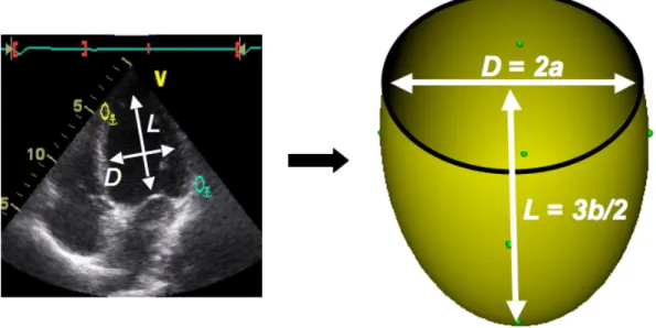
To describe the rapid filling phases, this resistance is considered lower during the diastole (Rmin) and higher
312
during systole (Rmax). A resistive law relates pressure and flow:
313
€
Q = Pc− Ps
R (17)
314
It is also necessary to take into account the blood mass effects which bring some inertial properties. So a 315
hydraulic inertance I can be introduced in order to define the law: 316
€
Pc− Ps= I
dQ
dt (18)
317
To summarize, each ventricular segment is modeled by four distinct entities for the electrical, mechanical, 318
mechano-hydraulic coupling and hydraulic parts. Each part is composed of the equations previously 319
described and some input-output relations. The links between the different parts of the segment model are 320
graphically described in figure 4. 321
322
Figure 4: Model of each ventricular segment. The mechanical model is connected to the electrical model and the mechano-hydraulic coupling 323
entity respectively through a simplified calcium concentration ([Ca2+]) representation, the radial force (F) and velocity (dr/dt). The hydraulic 324
model is linked to the mechano-hydraulic coupling entity and to the other segments respectively through the wall surface pressure (Ps), the 325
flow (Q), and the pressure at the center of the cavity (Pc). 326
327
Segments are also connected through the hydraulic domain (figure 5) as the total flow
€
Qtis the sum of the 328 regional flows € Qi: 329 € Qt = Qi i
∑
(19) 330The connections between the three layers are defined by considering the resistive properties of the blood 331
inside the cavity. 332
333
Figure 5: The twelve segments are connected in the hydraulic domain by adding each segment’s flow and by supposing that the pressures are 334
equal at the center of each layer. 335
336
The preload has been modeled by a constant flow source connected to a time-varying elastance that describes 337
the atrial behavior [54]: 338 € Ea= Emax− Emin 2 (1 − cos( π .tea Tmax )) + Emin 0 ≤ tea≤ 2.Tmax Emin 2.Tmax≤ tea≤ T ( 20 ) 339 340 where €
tea corresponds to the time elapsed since atrial electrical activation. The afterload is described by a 341
Windkessel model composed of a capacity, a resistance and an inertance. The heart valves are represented by 342
non-ideal diodes that correspond to modulated resistances and the valvular plane is described by a linear 343
capacitance. 344
In summary, the ventricular model is based on an ellipsoidal geometry and is composed of twelve segments 345
which describe the different energy domains involved in cardiac function: i) the electrical activity is 346
described by a cellular automata network, ii) the mechanical-hydraulic model represents the influence of 347
both active and passive forces developed by each segment on the blood inside the cardiac cavity. The twelve 348
segments are differentiated by specific parameters characterizing their electrical and mechano-hydraulic 349
properties. 350
The values for most of the parameters describing the mechanical behavior (c1, c2, c3, c4, c5, Tref, Bo, B1, 351
nref, pC50ref, B2) have been taken from other studies [25, 52]. The parameter values controlling afterload
352
and preload (capacitance, resistance, inertance and elastance) have been taken from [54, 55]. Appendix B 353
presents all these parameter values. The other parameters values are determined by means of the 354
identification algorithm. These parameters include the mechanical activation period (Tmax), the maximum
355
activation level (K) and the RDP period, for each segment. 356
Figure 6 presents the simulation of overall hemodynamic variables: ventricular pressure, flow and volume 357
for a normal cardiac cycle. Parameters for cellular automata have been fixed to fit electrical activation 358
patterns from [51]. The activation duration is equal to 400ms [26] and the maximum level of calcium 359
concentration is fixed at 7 µM [27]. 360
361
Figure 6: I) Stable resting left ventricular pressure-volume loop acquired from a human. The figure has been reproduced with permission from 362
[65], II) Model simulation of ventricular hemodynamic variables for one beat: A) intra-ventricular pressure B) aortic flow C) volume D) 363
pressure-volume loop. 364
365
Figure 7 shows simulated strains in basal and equatorial segments for a normal and a pathologic case. The 366
simulation of one cardiac cycle (800 ms of simulation), takes about 20s on a dual-core Intel Xeon 2.66Ghz. 367
368
The normal case (figure 7A) is simulated by using the same parameters as those used in figure 6. A 369
pathologic condition has been simulated by applying an additional electrical activation delay of 50 ms to the 370
anterior basal segment (figure 7B). The consequences of this regional desynchronisation can be observed on 371
the simulated strains during the isovolumic contraction phase, as the normal activation of the other 372
myocardial segments has produced an extension of the delayed segment. This phenomenon is marked with a 373
circle in figure 7B. 374
375
Figure 7: Strain simulation in healthy (left panel) and pathologic (right panel) conditions. The pathologic case was simulated by applying an 376
electrical activation delay of 50 ms on the anterior basal segment. The extension of the delayed segment can be observed for the pathologic 377
case during the isovolumic contraction phase (marked with a circle). 378
379
3.2. Model adaptation to experimental data
380
The model-based process, which is applied to the interpretation of strain morphology, is presented in figure 381
8. The whole process is composed of three main steps: i) acquisition of strain signals measured by TDI, ii) 382
adaptation of the model’s geometrical shape to real dimensions, determined by echocardiography and the 383
identification of patient-specific parameter values to reproduce the observed strain and iii) the physiological 384
interpretation of the identified parameters. This model-based approach is based on studies completed by our 385
laboratory which led to patient-specific parameter identification methods with applications in cardiology [50] 386
or epileptology [56]. 387
388
Figure 8: Parameters adaptation process. The evaluation of the error between observable signals and simulations is minimized in order to 389
determine the model’s parameters using an identification algorithm. The parameter values are representative of the physiological system state 390
and can help to interpret observations. 391
392
Concerning the adaptation of the geometrical shape, echocardiography reports usually inform us of the 393
ventricle’s length (L) and diameter (D). The model’s ellipsoid dimensions are defined from this data. In fact, 394
if the diameter is supposed to be measured at the equator, the minor axis can be computed as a = D/2. 395
Additionally, a relation between the major axis and the ventricle length is defined in [57] as b = 2L/3 (figure 396
9). Since the major and minor axes are known, it is possible to calculate, for each segment, the surface (S) 397
and the radii of curvature in order to get coefficients
€ Kθ, € Kϕ, € Kr. 398
399
Figure 9: Ellipsoidal model dimensions obtained from echocardiographic measures: a and b are respectively the minor and major axis sizes. 400
401
The identification algorithm is used to minimize the difference between experimental and simulated strains 402
on the eight myocardial segments at the base and at the equator. Parameters related to the four apical 403
segments have not been identified, as the strain data from these segments are difficult to acquire. For these 404
apical segments, the model parameters have been fixed from mean physiological values. These values are 405
listed in appendix 2. 406
3.2.1. Identification algorithm
407
The parameter identification can be seen as an optimization problem consisting of minimizing, for each beat 408
i, an error function defined as the difference between the synthesized strains and the observed strains. The
409
synthesized strains are obtained by simulating the proposed model M with a specific set of parameter values 410 P, such that: 411 € Xs obs = Strains obs(t) 412 € Xssim = Strains sim (t) = M (P) 413 where € Xsobs and €
Xssim represent, respectively, the observed and simulated strains for segment s and 414
€
t =
[
τQRSi,...,τQRSi +1]
where€
τQRSi represents the QRS detection instant for beat i. 415
The parameter set P defines the following values for each segment: the mechanical activation period (Tmax),
416
the maximum activation level (K) and RDP period ([RDP_segment, K_ segment , T_ segment]). Additionally, two
417
hydraulic resistance values are determined at the base and the equator ([R_max_base, R_min_base, R_max_equateur,
418
R_min_equateur]). In total, 28 parameters have to be identified and P is defined as P=[ R_max_base, R_min_base,
419
R_max_equateur, R_min_equateur, RDP_ant_base, RDP_inf_base, RDP_lat_base, RDP_septum_base, RDP_ant_equa,
420
RDP_inf_equa, RDP_lat_equa, RDP_septum_equa, K_ant_base, K_inf_base, K_lat_base, K_septum_base, K_ant_equa, K_inf_equa,
421
K_lat_equa, K_septum_equa, T_ant_base, T_inf_base, T_lat_base, T_septum_base, T_ant_equa, T_inf_equa, T_lat_equa,
422
T_septum_equa]. The objective is thus to obtain an optimal set of patient-specific parameters P* which
minimize an error function between € Xs obs and € Xs
sim. This error function has been defined here as the sum of 424
the absolute values of the difference between each experimental and simulated strain, calculated for the 425
whole cardiac cycle and for the 8 basal and equatorial segments. 426 € ε= Strains sim (t) − Strains obs (t) t=τQRSi τQRSi+1
∑
s=1 8∑
( 21 ) 427This error function is not differentiable and can have multiple local optima. This kind of problem can be 428
solved using Evolutionary Algorithms (EA), which are an adapted method used in identifying complex 429
nonlinear problems characterized by a poorly-known state-space. EA are stochastic search techniques, 430
inspired by the theories of evolution and natural selection, which can be employed to find an optimal 431
configuration for a given system within specific constraints [58]. 432
In these algorithms, the set of parameters P characterizes each "individual" of a "population". In order to 433
reduce the search space, values for parameters were bounded to the physiologically plausible intervals: [0.5 434
5] for the maximum hydraulic resistances, [0.01 0.5] for the minimum hydraulic resistances, [0.3 0.9] for 435
calcium period, [5 12] for calcium amplitude and [1 500] for electrical time activation. These intervals have 436
been defined around parameter values used for the simulation of global hemodynamic variables in section 437
3.1.5 (taken from other studies) and are based on physiological knowledge on the electromechanical 438
activities of the heart. 439
An initial population is created from a set of randomly generated individuals. The 28 parameter values of a 440
given individual are independently generated from a uniform distribution, defined under the corresponding 441
feasibility interval. This population will "evolve", minimizing the error function, by means of an iterative 442
process (figure 10). 443
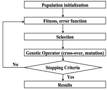
444
Figure 10: Working principles of evolutionary algorithms. A population is firstly initialized. The iterative procedure includes the evaluation of 445
the error function, individual selection and the creation of a new population using genetic operators. The process is applied until it reaches the 446
Once the error function has been evaluated for each individual, a new generation is produced by applying 448
mutation and crossover operators on selected individuals. The selection is carried out by means of the 449
"roulette wheel" method, adapted for function minimization, in which the probability of selecting a given 450
individual depends on the value of its error function, divided by the sum of all the error values of the 451
population. Only standard genetic operators, defined for real-valued chromosomes, have been used in this 452
work: "uniform crossover", which creates two new individuals (offspring) from two existing individuals 453
(parents), by randomly copying each allele from one parent or the other, depending on a uniform random 454
variable and "Gaussian mutation", which creates a new individual by randomly changing the value of one 455
allele (selected randomly), based on a Gaussian distribution around the current value. More details on these 456
kinds of optimization methods can be found on [59-61]. 457
4. Results and Discussion
458
4.1. Acquisition protocol
459
Strain acquisition using color tissue Doppler imaging has been applied to two healthy subjects and one 460
patient affected with dilated cardiomyopathy (DCM). This pathology is characterized by a heart enlargement 461
and a reduced mechanical cardiac function. Ultrasound measurements were performed in order to determine 462
the LV dimensions on two cardiac cycles. 463
For the two healthy subjects and the pathologic patient, the minor (a) and major (b) axes values are first 464
determined from echocardiography (Erreur ! Source du renvoi introuvable.). Dimensions for the 465
pathologic patient are particularly high, which is coherent with the diagnosis of a DCM. 466
467
Healthy Healthy DCM minor axis a 1.9725 1.8575 3.22
major axis b 4.8067 4.8033 5.99 Table 1: Minor (a) and major (b) axis values for the three patients.
468 469
4.2. Comparison between simulated and experimental strain
470
Strain signals have been measured on eight segments of the myocardial wall at the base level (the septum 471
and the anterior, inferior and lateral wall) and the equatorial level (the septum and the anterior, inferior and 472
lateral wall). In fact, it is not possible to obtain accurate data on the apical segments using TDI. Figure 11 473
shows simulations obtained after parameter adaptation and the clinically recorded strain signals for the three 474
subjects under study. The mean error value (calculated on the eight segments as presented in equation 21) is 475
equal to 2.4%, 2.09% and 1.30% respectively for the two healthy subjects and the pathologic patient, despite 476
the important disparity on the data from each subject. 477
478
Figure 11: Comparison between simulated and experimental strains for the two healthy subjects and the pathologic patient during one cardiac 479
cycle for the septum, anterior, inferior and lateral walls of the base and equator. The continuous curve is the simulation and the segmented one 480
is the experimental data. The strain is expressed as a percentage of the diastolic state. 481
482
Simulated systolic peak times are coherent with the observation and the reproduction of the overall 483
morphology of the isovolumic contraction and systolic phases is approached with relative errors of 2.12%, 484
2.16% and 1.25% for the first, second and third subject, respectively. Additionally, the simulations reproduce 485
some particularities that are due to the pathology. In fact, for the patient suffering from DCM, positive values 486
on some strain signals can be observed during the isovolumic contraction. These strain elevations are due to 487
increased electrical activation delays in the corresponding segments and they can be explained by the 488
extension of yet inactivated segments during the contraction of the other segments. This example shows how 489
the model-based approach may assist in the interpretation of myocardial strain morphologies. 490
491
4.3. Interpretation of the identified parameters
492
The previous results can be represented graphically by visualizing the deformations which have been applied 493
to the twelve myocardial segments at each time step. Simulated strains, obtained using patient-specific 494
parameters, are applied at the center of the corresponding myocardial segment. The cardiac surface 495
The surface is represented by a graph on which are defined landmarks (data points). The position of each 497
landmark being known during the whole cardiac cycle, the cardiac surface deformation is computed using 498
TPS interpolation (based on a bending energy, defined as the integral, over all the mesh nodes, of the squares 499
of the second derivatives). Figure 12 shows the ventricular deformation and the identified electrical activity 500
for the three subjects during the cardiac cycle. The electrical activation sequences for the two healthy 501
subjects are coherent with well-known activation maps [51]. It possible to observe a reduced mechanical 502
activity and a delayed electrical activation on the DCM patient. A qualitative evaluation of the three 503
simulated sequences has been performed by a cardiologist. He confirms that simulations correspond to 504
pathophysiologically plausible sequences. The delayed electrical activity observed in the simulation for the 505
DCM patient can be explained by an intra-ventricular desynchronisation, frequently observed in this kind of 506
pathology. A quantitative evaluation of the estimated activation sequence could be performed by acquiring 507
an electrophysiological cartography for each patient. This delicate invasive procedure has not been applied 508
for the patient analyzed in this paper. However, this kind of evaluation will be possible using data acquired 509
on a current clinical protocol running at the Rennes University Hospital. 510
511
Figure 12: Contraction of the electromechanical model for the two healthy subjects and the pathologic patient. The color legend corresponds to 512
the electrical state of each segment and is expressed in mV. The orientation of the ventricular model is depicted in the lower right panel of the 513
figure. 514
515
The identification process brings patient-specific parameters that are interesting to analyze, since they can be 516
representative of the physiopathological state. To facilitate the visualization of these results, the “Bull’s eye” 517
representation is used to depict the electro-mechanical parameters identified for each segment (figure 13). 518
519
Figure 13: Bull’s eye representation of ventricular parameters. For each Bull’s eye diagram, the left, top, right and down parts represent the 520
septal, anterior free wall and posterior regions, respectively. The outer, mid- and inner rings represent the base, the equator and the apex of the 521
LV. This representation will be used in figures 14 and 15. 522
523
Figure 14 shows the electrical activation times for the three patients. The maximum values reach 54 ms, 67.4 524
ms and 126 ms for the first and second subjects and the DCM patient, respectively. It is easy to verify that 525
the pathologic patient presents increased electrical activation delays in comparison with well-known 526
activation maps [51]. 527
The mechanical activity peak time
€
TMP can also be analyzed. In order to compare this parameter for the three 528
patients, the identified
€
TMP is expressed as a percentage of the cardiac cycle duration (RR interval): 529
€
TMP%= 100.TMP RR
530
Figure 15 shows the bull’s eye representation of identification results. For the first healthy subject, the 531
mechanical activity peak time goes from 18% to 37% of the RR interval. For the second one, this parameter 532
varies from 21% to 37%.
€
TMP% ranges from 31% to 60% for the affected patient. 533
534
Figure 14: Bull’s eye representation of the electrical activation times (TAE) for the two healthy subjects and the pathologic patient. The 535
maximum values reach 54 ms, 67.4 ms and 126 ms respectively for the first, second subject and the pathologic patient. 536
The
€
TMP% comparison for both healthy subjects shows similar value ranges. The third patient percentages 539
are higher overall. These values are particularly high for the anterior and lateral segments of the base because 540
they are respectively equal to 60 % and 55 %. The increased
€
TMP% is a marker of a myocardial dysfunction 541
concerning these two segments. The model-based localization of the delayed segments and the magnitude of 542
the desynchronization for the DCM patient are in accordance with the diagnosis provided by the expert 543
cardiologist. Moreover, the model-based approach provided further insight in the explanation of the observed 544
strain morphologies. 545
546
Figure 15: Bull’s eye representation of the mechanical activity peak time expressed as a percentage of the RR-interval (TMP%) for the two 547
healthy subjects and the pathologic patient. These values are high for the anterior and lateral segments of the DCM patient. 548
4.4. Robustness analysis
549
In order to test the robustness of the identification method, the algorithm has been repeated ten times on one 550
subject. Figure 16 shows boxplots of the identified
€
TMP parameters. The results of the ten identifications are
551
close enough to show that the parameter interpretation is available from a physiological point of view. 552
Furthermore, it can be seen from these box-plots, and from results in section 4.3, that the identified 553
parameter values do not reach the upper or lower boundaries of the physiological plausible intervals defined 554
in section 3.2.1. 555
556
Figure 16: The identification algorithm has been repeated ten times on one subject in order to test the robustness of the identified parameters. 557
This figure shows the boxplot of the ten identified
€
TMP for the first healthy subject.
558
4.5. Study Limitations
559
The main limitations of the proposed approach are related to the hypotheses made to build the ventricular 560
model, the observability of TDI strain analysis, and the current clinical evaluation state. 561
Concerning the ventricular model, the following hypotheses were made in order to obtain a tissue-level, 562
lightweight model on which we could perform parameter identification from observed strain signals: i) the 563
ventricular torsion motion has been neglected, ii) the mechanical continuity between segments is not always 564
assured, as the ventricle is represented by a set of sub-pumps coupled in the hydraulic domain and 565
commanded by a coordinated electrical activity, iii) the intracellular calcium concentration is approximated 566
by an analytic expression and iv) the myocardial fiber orientation is assimilated to a mean angle. Although 567
these simplifications have a direct consequence on the synthesis of strain signals, in particular during the 568
diastolic period (as discussed above), the authors consider that they are in accordance to the problem under 569
study and the resulting model can already be useful to assist in the interpretation of strain data. 570
Another limitation concerns the limited observability of the apical segments from strain analyses. As already 571
mentioned, in order to overcome this problem, the model parameters for the apical segments have been fixed 572
from mean physiological values and are not included into the identification process. 573
Finally, concerning the clinical evaluation of the approach, only a limited number of healthy subjects and 574
DCM patients have been analyzed so far. Although these results are encouraging and show the feasibility of 575
the approach, a larger clinical evaluation is necessary in order to validate the interpretations obtained from 576
this model-based approach. 577
5. Conclusion
579
The present paper described a model-based approach for the analysis of myocardial strain data. The method 580
is based on a tissue-level model of the left ventricle that includes a simplified geometrical representation, a 581
description of the electrical, mechanical and hydraulic activities and a physiological segmentation, which are 582
in accordance to the problem under study. As low computational resources are required for the simulations 583
of the proposed model, the identification of patient-specific parameters becomes feasible. 584
Patient-specific parameters were obtained for two normal subjects and one patient suffering from DCM. The 585
mean error between observed and synthesized strain signals, after parameter identification, is particularly 586
low (between 1.30% and 2.34%). A qualitative comparison between the results obtained from the proposed 587
model-based approach and a classical TDI analysis has been performed by a cardiologist/echocardiographer 588
(ED). The localization of failing segments and the values and instants of occurrence of the peak systolic 589
strains have shown to be coherent with the clinical analysis. The model also allows a better reproducibility in 590
the estimation of systolic peaks and adds the possibility of estimating electrical activation times, which are 591
difficult to observe experimentally. This appears particularly useful as echocardiographic strain signals are 592
sometimes noisy and challenging to interpret, limiting its large use in routine clinical practice. Recent papers 593
insist on this problem of reproducibility and robustness of the echocardiographic interpretation (PROSPECT 594
study [63] and RETHINQ study [64]). 595
Moreover, such a patient-specific model-based method can be used to assist the interpretation of strain 596
morphologies and to find, via simulations, the origin of particular strain shapes. The main advantage of this 597
model-based approach with respect to “black-box” approaches, such as neural networks, is that the patient-598
specific parameters characterizing the model provide a direct physiological interpretation. Due to this 599
property, these model-based approaches can be useful for a better interpretation of the morphology of strain 600
signals and to assist diagnosis and therapy definition. 601
Current work is directed towards the improvement of the ventricular model and a further clinical evaluation 602
of the proposed approach. In this sense, a clinical protocol including electrophysiological cartography, TDI 603
and multi-slice computer tomography on patients receiving cardiac resynchronization therapy is currently in 604
progress in the Rennes University Hospital (IMOP project). 605
Acknowledgements
606
The authors would like to thank Antoine Simon for his valuable assistance in the exploitation of the 607
visualization tools. 608
6. Appendix A
609
The strain ε is a mechanical expression reflecting the percentage deformation of a given myocardial segment 610
with respect to its original end-diastolic state and can be defined as: 611
€
ε = l − L
L ( 22 )
612
where l is the current length of the object and L its original length. The main concepts of TDI acquisition and 613
analysis are explained in [1, 2]. Briefly, the instantaneous change in length (dl) of a given object can be 614
obtained from the estimation of the velocity of two different points at the end extremity of the object of 615 interest (v1 and v2), as 616 € dl = (v1− v2)dt ( 23 ) 617
This quantity can be divided by L in order to obtain the velocity gradient, or strain rate SR, which is thus 618 defined as: 619 € dl l = v1− v2 l dt ( 24 ) 620
As it is difficult to obtain the velocity of two points at the extremities of the object, the velocity gradient is 621
estimated from two points separated by a fixed distance (Δr) and equation 25 becomes 622 € dl l ≈ v(r) − v(r + Δr) Δr dt ( 25 ) 623
Equation 26 is integrated to obtain: 624 € logl L= toSR t
∫
dt ( 26 ) 625where log is the natural logarithm. The expression of strain can be deduced from the last equation: 626 € ε= exp( SR to t
∫
dt) −1 ( 27 ) 627Myocardial strain estimation from TDI measurements are performed in practice as follows: The operator 628
manually identifies one to six regions of interest and the software will automatically define two sets of points 629
spaced from 9 to 12 mm within the defined region of interest. The software will then compare the velocity 630
vectors of these two sets of points during a cardiac cycle to calculate strain and strain rate. It is important to 631
note that the strain acquisition depends on the ultrasound beam orientation and the axis of the left ventricle. 632
7. Appendix B
633
Table 2 presents the model parameter values, extracted from other studies, which have been left fixed on the 634
model (not identified), as well as their sources. 635
636 637
637 638 639 640 641 642 643 644 645 646 647 648 649 650 651 652 653 654 655 Table 2: 656 Model parameter values. 657 658
Parameters Values Source Preload Sf 25 ml/s Estimated Atria Emin 1.2 mmHg/ml [56] Emax 0.06 mmHg/ml [56] T 0.12 s [56] Afterload R 3 mmHg.s/ml [24] C 0.219 ml/mmHg [40] I 0.00082 mmHg.s2/ml [40] Valve Rpass 0.01 mmHg.s/ml Estimated Rblo 100 mmHg.s/ml Estimated VENTRICLE Valvular Plan C 0.05 ml/mmHg Estimated Hydraulic Résistance T1 0.03 s Estimated T2 0.05*RR s Estimated Inertance I 0.0001 mmHg.s2/ml Estimated Geometric Parameters Mean fibre angle with respect to
the equatorial plane
π/12 [52] Thickness 1 cm [52] Active Properties Tref 940 mmHg [32] B0 1.45 [32] B1 1.95 [32] n_ref 4.25 [32] pC50_ref 5.33 [32] B2 0.31 [32] Passive Properties C1 113.9 mmHg [10] C2 550.71 mmHg [10] C3 10.5 mmHg [10] C4 -146.1 mmHg [10] C5 141 mmHg [10]
659
8. References
660
[1] J. D'Hooge, A. Heimdal, F. Jamal, T. Kukulski, B. Bijnens, F. Rademakers, L. Hatle, P. Suetens, and 661
G. R. Sutherland, "Regional strain and strain rate measurements by cardiac ultrasound: principles, 662
implementation and limitations," European Journal of Echocardiography, vol. 1, pp. 154-70, 2000. 663
[2] S. Urheim, T. Edvardsen, H. Torp, B. Angelsen, and O. A. Smiseth, "Myocardial strain by Doppler 664
echocardiography. Validation of a new method to quantify regional myocardial function," 665
Circulation, vol. 102, pp. 1158-64, 2000.
666
[3] A. Heimdal, A. Stoylen, H. Torp, and T. Skjaerpe, "Real-time strain rate imaging of the left ventricle 667
by ultrasound," Journal of the American Society of Echocardiography, vol. 11, pp. 1013-9, 1998. 668
[4] E. Donal, P. Raud-Raynier, D. Coisne, J. Allal, and D. Herpin, "Tissue Doppler echocardiographic 669
quantification. Comparison to coronary angiography results in Acute Coronary Syndrome patients," 670
Cardiovascular Ultrasound vol. 3, pp. 10, 2005.
671
[5] T. Kukulski, F. Jamal, L. Herbots, J. D'Hooge, B. Bijnens, L. Hatle, I. De Scheerder, and G. R. 672
Sutherland, "Identification of acutely ischemic myocardium using ultrasonic strain measurements. A 673
clinical study in patients undergoing coronary angioplasty," Journal of the American College of 674
Cardiology, vol. 41, pp. 810-9, 2003.
675
[6] T. Edvardsen, B. L. Gerber, J. Garot, D. A. Bluemke, J. A. Lima, and O. A. Smiseth, "Quantitative 676
assessment of intrinsic regional myocardial deformation by Doppler strain rate echocardiography in 677
humans: validation against three-dimensional tagged magnetic resonance imaging," Circulation, vol. 678
106, pp. 50-6, 2002. 679
[7] P. Claessens, Claessens C. , Claessens J. , Claessens M. , "Strain Imaging: Key to the Specific Left 680
Ventricular Diastolic Properties in Endurance Trained Athletes," Journal of Clinical and Basic 681
Cardiology, vol. 6, pp. 35-40 2003.
682
[8] M. Guarini, J. Urzua, A. Cipriano, and W. Gonzalez, "Estimation of cardiac function from computer 683
analysis of the arterial pressure waveform," IEEE Transactions on Biomedical Engineering, vol. 45, 684
pp. 1420-8, 1998. 685
[9] J. L. Palladino and A. Noordergraaf, "A paradigm for quantifying ventricular contraction," Cellular 686
and Molecular Biology Letters, vol. 7, pp. 331-5, 2002.
687
[10] A. L. Hodgkin and A. F. Huxley, "A quantitative description of membrane current and its 688
application to conduction and excitation in nerve," Journal of Physiology, vol. 117, pp. 500-44, 689
1952. 690
[11] G. W. Beeler and H. Reuter, "Reconstruction of the action potential of ventricular myocardial 691
fibres," Journal of Physiology, vol. 268, pp. 177-210, 1977. 692
[12] C. H. Luo and Y. Rudy, "A dynamic model of the cardiac ventricular action potential. II. 693
Afterdepolarizations, triggered activity, and potentiation," Circulation Research, vol. 74, pp. 1097-694
113, 1994. 695
[13] R. L. Winslow, J. Rice, S. Jafri, E. Marban, and B. O'Rourke, "Mechanisms of altered excitation-696
contraction coupling in canine tachycardia-induced heart failure, II: model studies," Circulation 697
Research, vol. 84, pp. 571-86, 1999.
698
[14] R. A. FitzHugh, "Impulses and physiological states in theoretical models of nerve membrane," 699
Biophysical Journal, vol. 1, pp. 445–466, 1961.
700
[15] A. L. Bardou, P. M. Auger, P. J. Birkui, and J. L. Chasse, "Modeling of cardiac electrophysiological 701
mechanisms: from action potential genesis to its propagation in myocardium," Critical Reviews™ in 702
Biomedical Engineering, vol. 24, pp. 141-221, 1996.
703
[16] P. Colli Franzone, Pavarino L.F. and Taccardi B. , "Monodomain Simulations of Excitation and 704
Recovery in Cardiac Blocks with Intramural Heterogeneity," Funcional Imaging and Modeling of 705
the Heart (FIMH), pp. 267–277, 2005.
706
[17] C. S. Henriquez and R. Plonsey, "Simulation of propagation along a cylindrical bundle of cardiac 707
tissue--I: Mathematical formulation," IEEE Transactions on Biomedical Engineering, vol. 37, pp. 708