Design and Development of a 3D X-ray Microscope
by
Jordan B. Brayanov
B.S. Electrical Engineering and B.S. Mechanical Engineering
MIT, 2004
Submitted to the Department of Mechanical Engineering in Partial Fulfillment of the
Requirements for the Degree of
Master of Science in Mechanical Engineering
at the
Massachusetts Institute of Technology
February, 2006
©2006 Massachusetts Institute of Technology
All Rights Reserved
Signature of Author ...
-- - -7 - ... Depa4 fieif Mechanical Engineering January 20, 2006C ertified by ...
...
Ian W. Hunter Hatsopoulos Professor of Mechanical Engineering and Professor Biological Engineering Thesis Supervisor
Accepted by ...
Lallit Anand
SSACHUSETTS INS TUTE Professor of Mechanical Engineering
Chairman, Department Committee on Graduate Students
MA
- I
M
ITLibraries
Document Services Room 14-0551 77 Massachusetts Avenue Cambridge, MA 02139 Ph: 617.253.2800 Email: [email protected] http://libraries.mit.edu/docsDISCLAIMER NOTICE
The accompanying media item for this thesis is available in the MIT Libraries or Institute Archives.
Design and Development on a 3D X-ray Microscope
byJordan B. Brayanov
Submitted to the Department of Mechanical Engineering
on January 2 0th, 2006 in Partial Fulfillment of the Requirements for the Degree of Master of Science in Mechanical Engineering
ABSTRACT
The rapid development of needle-free injection systems demands better and faster imaging systems, capable of imaging the transient and steady state response of an injection into real tissue. X-ray radiography, x-ray microscopy, and computerized tomography (CT) were identified as the most appropriate imaging techniques used for non-invasive imaging of opaque objects and an instrument was constructed, utilizing all of those techniques.
The instrument was capable of producing x-ray radiographies with native resolution of less than 30 pm, frame rate of 32 frames per second and a field of view of 30 mm by 40 mm. Using magnifying cone-beam x-ray source the ultimate resolution of the system exceeded 5 pm, while maintaining image sharpness and clarity. Digital image
reconstruction techniques, based on the inverse Radon transformation and the Fourier slice theorem were used to regenerate conventional CT images as well as contrast volumetric 3D images of the internal structures of opaque objects.
This paper presents the design and development of the 3D x-ray microscope together with experimental results obtained during the calibration and initial testing of the
instrument.
Thesis Supervisor: Ian W. Hunter
Table of Contents ABSTRACT 2 TABLE OF CONTENTS 3 LIST OF FIGURES 6 LIST OF TABLES 9 ACKNOWLEDGEMENTS 10
1. INTRODUCTION AND MOTIVATION 11
2. HISTORICAL BACKGROUND 12
2.1. X-RAY RADIOGRAPHY 12
2.2. CONVENTIONAL X-RAY TOMOGRAPHY 15
2.3. COMPUTED X-RAY TOMOGRAPHY 17
2.4. EVOLUTION OF CT SCANNERS 19
2.4.1. FIRST GENERATION CT SCANNER 19
2.4.2. SECOND GENERATION CT SCANNER 20
2.4.3. THIRD GENERATION CT SCANNER 21
2.4.4. FOURTH GENERATION CT SCANNER 22
2.4.5. FIFTH GENERATION CT SCANNER 23
3. THEORETICAL FUNDAMENTALS 25
3.1. MATHEMATICS FUNDAMENTALS 25
3.1.1. LINEAR ALGEBRA 25
3.1.2. FOURIER ANALYSIS 29
3.2. FUNDAMENTALS OF X-RAY PHYSICS 31
3.2.1. GENERATION OF X-RAYS 31
3.2.2. X-RAYS - MATTER INTERACTIONS 33
3.2.3. RADIATION DOSE 36
4. IMAGE PROCESSING 39
4.1. IMAGE RECONSTRUCTION 39
4.1.1. LINE INTEGRAL MEASUREMENTS 39
4.1.2. ALGEBRAIC RECONSTRUCTION TECHNIQUE 41
4.1.4. THE FOURIER SLICE THEOREM 45 4.1.5. FAN BEAM RECONSTRUCTION 50
4.2. IMAGE ENHANCEMENT 53
4.2.1. HISTOGRAM TRANSFORMATIONS 54
4.2.2. IMAGE AVERAGING 56
4.2.3. MEDIAN FILTERING 58
4.2.4. IMAGE SHARPENING AND EDGE ENHANCEMENT 59
4.3. IMAGE MAGNIFICATION 61
4.4. IMAGE VISUALIZATION 63
4.4.1. TRADITIONAL CT IMAGE VISUALIZATION 63
4.4.2. VOLUMETRIC VISUALIZATION 65
5. X-RAY MICROSCOPE DESIGN 67
5.1. FUNCTIONAL COMPONENTS 68
5.2. STRUCTURE 68
5.3. MECHANICS 71
5.4. ELECTRONICS 73
5.5. SOFTWARE 74
5.5.1. X-RAY SOURCE CONTROL SOFTWARE 75
5.5.2. ROTARY STAGE CONTROL SOFTWARE 76
5.5.3. IMAGE ACQUISITION SOFTWARE 76
5.5.4. IMAGE RECONSTRUCTION SOFTWARE 76
5.6. DESIGN SUMMARY 77
6. X-RAY MICROSCOPE IMPLEMENTATION 79
6.1. FUNCTIONAL COMPONENTS 79
6.1.1. DIGITAL CCD IMAGING CAMERA 79
6.1.2. X-RAY SOURCE 80
6.2. STRUCTURE 81
6.3. ELECTRONICS 82
6.4. MECHANICS 87
6.5. SOFTWARE 88
6.5.2. ROTARY STAGE CONTROL SOFTWARE 90
6.5.3. IMAGE ACQUISITION SOFTWARE 91
6.5.4. IMAGE RECONSTRUCTION SOFTWARE 93
6.5.4.1 .TWO-DIMENSIONAL RADIOGRAPHY GENERATION 94
6.5.4.2.CONVENTIONAL 3D CT IMAGE GENERATION 95
6.5.4.3.VOLUMETRIC 3D CT IMAGE GENERATION 96
6.6. COMPLETE SYSTEM OVERVIEW 96
7. RESULTS AND DISCUSSION 97
7.1. CALIBRATION 97 7.1.1. LEAD ENCLOSURE 97 7.1.2. X-RAY SOURCE 98 7.1.3. DIGITAL CCD CAMERA 99 7.1.4. MICROSCOPE MAGNIFICATION 102 7.2. TWO-DIMENSIONAL RADIOGRAPHS 104
7.3. CONVENTIONAL 3D TOMOGRAPHIC IMAGES 106
7.4. VOLUMETRIC 3D TOMOGRAPHIC IMAGES 111
8. CONCLUSIONS AND FUTURE WORK 113
BIBLIOGRAPHY 115
APPENDIX A: EQUIPMENT SPECIFICATIONS 118
APPENDIX A. 1: CAMERA SPECIFICATIONS 118
APPENDIX A.2: X-RAY SOURCE SPECIFICATIONS 119
APPENDIX A.3: POWER SUPPLY SPECIFICATIONS 120
APPENDIX B: SOFTWARE 121
APPENDIX B.1: SOURCE CODE FOR ROTARY STAGE CONTROL 121
APPENDIX B.2: IMAGE ENHANCEMENT GUI 126
APPENDIX B.3: SOURCE CODE FOR CONVENTIONAL CT RECONSTRUCTION 130
List of Figures
Figure 2.1: Sample radiographs of human hands. 13
Figure 2.2: Early 1900s radiographic system. 13
Figure 2.3: Radiographic system using fluorescent screen. 14
Figure 2.4: Shoe fitting X-ray device. 14
Figure 2.5: Principle of the first conventional tomography device. 15
Figure 2.6. Conventional tomography. 16
Figure 2.7: Hounsfield working on the first laboratory CT scanner. 18
Figure 2.8: Early clinical CT imaging. 19
Figure 2.9: First generation CT scanner. 20
Figure 2.10: Second generation CT scanner. 21
Figure 2.11. Third generation CT scanner. 22
Figure 2.12: Fourth generation CT scanner. 23
Figure 2.13: Fifth generation CT scanner. 24
Figure 3.1: Basic Fourier transform properties. 31
Figure 3.2: Electromagnetic spectrum. 33
Figure 4.1: Monochromatic x-ray attenuation. 40
Figure 4.2: A simple example of an object and its projections. 42 Figure 4.3: Illustration of algebraic reconstruction technique (ART). 43 Figure 4.4: Line integral projection P(p, 0) of the 2-D Radon transform. 45 Fgure 4.5: The Fourier Slice theorem relates the Fourier transform of a projection to
47 the Fourier transform of the object along a radial line.
Figure 4.6: Sampling pattern in frequency domain based on Fourier slice theorem. 50
Figure 4.7: Different fan beam geometries. 51
Figure 4.8: Fan beam projection pattem. 51
Figure 4.9: Projection patterns for different beam geometries. 52
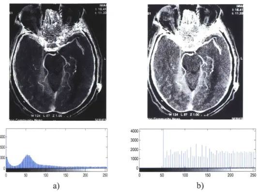
Figure 4.10: Sample brain CT image with histogram equalization. 55 Figure 4.11: Sample brain CT image with spatial averaging. 57
Figure 4.13: Sample brain CT image with median filtering. 59
Figure 4.14: First-order gradient (Sobel filter) masks. 60
Figure 4.15: Sample brain CT image with Laplacian filtering. 61
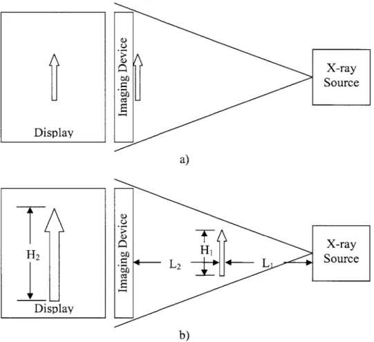
Figure 4.16: Magnification by using cone-beam x-ray source. 62
Figure 4.17: CT image of a human head. 64
Figure 4.18: Reconstructed "slice" images sequentially arranged in a "stack." 66
Figure 4.19: MPR image of a human lumbarosacral spine. 66
Figure 5.1: General system overview. 67
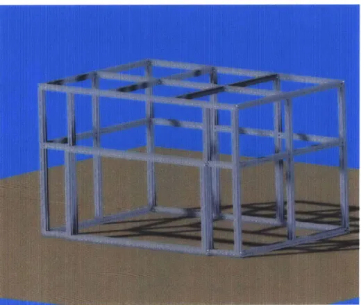
Figure 5.2: CAD model of aluminum support frame. 69
Figure 5.3: CAD model of lead enclosure with missing front panels 70
Figure 5.4: CAD model of main structure 71
Figure 5.5: Picture of mechanical safety interlock switches 72
Figure 5.6: Key mechanical components. 73
Figure 5.7: Main wiring diagram. 74
Figure 5.8: Major software components interactions. 75
Figure 5.9: Image reconstruction algorithm flow diagram 77
Figure 5.10: CAD model of complete system. 78
Figure 6.1: Hamamatsu C4742-56-12NR digital CCD camera setup. 80
Figure 6.2: Source Ray SB-80-500 x-ray source. 81
Figure 6.3: Aluminum support frame. 82
Figure 6.4: Lead shielded enclosure. 83
Figure 6.5: X-ray source support electronics. 84
Figure 6.6: Illumination. 85
Figure 6.7: Power supply enclosure. 86
Figure 6.8: Electrical safety components. 86
Figure 6.9: Mechanical interlock safety switch and counterweight system. 87
Figure 6.10: Rotary stage together with its stepper motor and drive. 88
Figure 6.11: X-ray source control software GUI. 89
Figure 6.12: Communication scheme used to control the rotary stage. 90
Figure 6.13: Rotary Stage Control software GUI. 91
Figure 6.15: HyperCam interface. 93
Figure 6.16: Flowchart of the entire image reconstruction process. 94
Figure 6.17: Image enhancing application. 95
Figure 6.18: Picture of complete system. 96
Figure 7.1: Results from the cooling system evaluation test. 98
Figure 7.2: Image histogram 99
Figure 7.3: Noise distribution analysis for V=40 kV 100
Figure 7.4: Noise distribution analysis for V=35 kV 100
Figure 7.5: Contrast test phantom. 101
Figure 7.6: Resolution test phantom. 102
Figure 7.7: Magnification test. 103
Figure 7.8: Images of DAC725JP microchip. 104
Figure 7.9: Images of 256 MB I-Stick USB Drive. 105
Figure 7.10: Endoscopic probe operating inside an opaque enclosure. 105 Figure 7.11: Radiography of simple cylindrical phantom. 106
Figure 7.12: Initial reconstruction attempt of conventional CT image. 107
Figure 7.13: Improved reconstruction of conventional CT image of needle phantom. 107
Figure 7.14: Solid stainless-steel phantom (lure-lock). 108
Figure 7.15: Reconstructed conventional CT image of lure-lock phantom. 109
Figure 7.16: Snail shell phantom. 109
Figure 7.17: 12 reconstructed layers of the snail shell phantoms. 110
Figure 7.18: Radiograph of the snail shell phantom. 111
List of Tables
Table 3.1: Summary of basic matrix properties 27
Table 3.2: Quality factors of various types of ionizing radiation. 37
Table 3.3: Radiation sensitivity of various organs. 38
Table 3.4: Effective Dose Equivalent HE for Clinical X-ray and CT Exams 38
Acknowledgements
I would like to express my gratitude to Professor Ian Hunter for the opportunity
he gave me to work on this project. I would also like to thank him for his support and encouragements in conducting this research and interpreting the results.
My gratitude extends to Dr. Andrew Taberner for helping me devise relevant
experiments and assisting me in resolving issues with the laboratory equipment and my experiments.
I would like to pay my sincere gratitude to my colleague Atanas "Nasko" Pavlov
and Andrea Bruno for their moral support and their insight in the subjects of x-ray physics and image processing.
I render my special thanks to my girlfriend Eleonora "Ellie" Vidolova for
generously giving me her time in editing my thesis and helping me with the visually appealing arrangement of this document.
Last, but not least, I would like to thank my friends Boyan Yordanov, Nayden Kamboushev, Iliya Tsekov, and Nikolay Andreev for proof-reading my thesis and providing me with invaluable feedback.
1. Introduction and Motivation
X-ray imaging has been a popular research topic for over a century in various scientific fields. Radiography, tomography, and microscopy systems using x-rays have been studied and carefully documented for decades; yet, with the development of new technologies and image processing algorithms, rapid improvement of existing instrumentation is not unusual.
Imaging system development usually follows along the development of new experimental techniques, which need to be observed and documented. Over the last few years we had been developing a novel Needle-Free Injection (NFI) system for both veterinary and human use and we had achieved most of our goals. However, due to limitations in the conventional imaging system we had been using to document our progress, it had been extremely difficult to document and present our success.
The purpose of our injection system was to inject fluids into live tissue. Since live tissue is opaque to visible light, injections could neither be observed, nor documented in real time and so we decided to use an x-ray based 3D microscopy system, which could image inside the tissue and record the effects of the injection.
Even though 3D x-ray microscopy systems were commercially available and could be customized to meet most of our specifications, their delivery time was between six and twelve month, which meant huge delays in our progress. Furthermore, all commercial systems had fixed architecture and were not easily reconfigurable, which was essential to any future experiments for which the system could be used.
The best option we had was to develop an instrument that would meet all our requirements and provide us with the imaging resources we desperately needed. We also decided to build the system flexible and modular, so that it could easily be upgraded or modified in the future as new experimental techniques were developed.
2. Historical Background
X-rays were first observed in the late 1800s by scientists around the world. In 1887 Nikola Tesla began investigating the unknown radiation produced by the high-voltage vacuum tubes he designed. Heinrich Hertz experimented and demonstrated in 1892 that cathode rays could penetrate very thin aluminum foil and later developed a cathode ray tube that would emit x-rays capable of penetrating various metals. However it was Wilhelm Rdntgen in November 1895 who first documented x-rays as a new type of radiation.
On December 2 8th 1985 R6ntgen wrote a preliminary report "On A New Kind of
Rays," which was the first formal recognition and categorization of x-rays. In this report
he referred to the rays as "X", indicating that they were unknown to the scientific society at that time. Wilhelm R6ntgen was awarded an honorary degree of Doctor of Medicine in
1896 and received the first Nobel Prize in Physics in 1901 for his discovery. He refused
to take any patents related to his discovery on moral grounds and did not even want the rays to be named after him. However, many of his colleagues started calling them
"R6ntgen rays," a term still in use in many countries.
2.1. X-ray Radiography
In parallel with the discovery of x-rays, Dr. R6ntgen was working on possible applications for them. He discovered that if an object of variable density is positioned between a cathode ray tube (an x-ray source) and a photographic film and irradiated with x-rays generated by the tube, a contrast image, called a radiograph, is produced. Figure 2.1 (a) shows a radiograph of Bertha Rdntgen's hand taken on November 8th 1895. The radiograph clearly shows the contrast between tissue, bone, and a metal ring and lays the foundation of 100 years of non-invasive medical imaging. Figure 2.1 (b) shows a radiograph taken by a modem x-ray imaging system, with much better soft tissue contrast. Nevertheless, Dr. Rbntgen's radiography is remarkable in retrospect.
Since Rbntgen's discovery that x-rays can be used identify bony structures, scientists all over the world began developing medical imaging devices based on x-rays. Figure 2.2 shows an early 1900s radiography system, in which the patients had to hold the film
while being irradiated. In the earliest days a chest x-ray would require up-to 10 minutes of exposure and a radiation dosage 50 times greater than that of a modem x-ray.
a) b)
Figure 2.1: Sample radiographs of human hands. a) Image of Bertha R6ntgen's hand, b) Image taken by a modern X-ray system.
[Images taken from Wikipedia, 2006]
In the early days of non-invasive medical imaging no one realized the danger posed
by prolonged exposure to x-rays. The matter became worse with the development of
fluorescent screens, shown in Figure 2.3, and special glasses, allowing doctors to see x-ray images in real time. This caused doctors to stare directly into the x-x-ray beam, creating unnecessary exposure to radiation.
Figure 2.2: Early 1900s radiographic system. [Image taken from Imaginis, 2006]
Figure 2.3: Radiographic system using fluorescent screen. [Image taken from Imaginis, 20061
In the commercial sector people started using x-rays for inspection, quality control, even shoe fitting. In the late 1940's a shoe fitting x-ray unit, similar to the one shown in Figure 2.4, was present in most show stores in the US. It was estimated that by the late 1950's over 10,000 of these devices were in use. It was in the 1950's when the radiation hazards associated with x-rays were first recognized and the first regulations were imposed over the use of x-rays.
Figure 2.4: Shoe fitting X-ray device. [Image taken from MQMD, 20061
Around the beginning of the 1920s people started to realize that they could not overcome the poor low-contrast resolution of conventional radiography. They also realized that they could not distinguish between structural layers of the subjects being studied, which led to the development of the conventional tomography.
2.2. Conventional X-ray Tomography
Conventional tomography, also known as body section radiography, was first suggested by Mayer in 1914. As early as 1921 Bocage, one of the pioneers of conventional tomography, described an apparatus which could blur structures above and below a plane of interest. The major components of his invention were an x-ray tube, a
film, and a mechanical coupling which allowed synchronous movement of the tube and
the film. The principle of this device is illustrated in Figure 2.5.
Source B
Focal Plane
A
Fihn
Figure 2.5: Principle of the first conventional tomography device. [Image taken from EPM, 2006]
The idea behind the device was simple: let us consider two distinct points inside a patient, A and B, and let point A lie on the focal plane and point B lie off the focal plane. As the film and the x-ray source move, the projection of point A onto the film stays the same (which is true for all point on the focal place), while the projection of point B changes to a different location on the film. This is due to the fact that point B is off the focal plane and the ratio of the distance from point B to the x-ray source and the distance from point B to the film deviates from that of the same distance ratio for point A. When
the x-ray tube and the film move continuously along a straight line, the shadow of point B forms a line segment instead of a point. This holds for all point above and below the focal plane. Therefore in the final image the highest intensity component would be produced by the point on the focal plane.
The first device based on that approach was successfully built in 1924. Devices using the same technology (with very minor changes) were used until the late 1960s. Figure 2.6 (a) shows a picture of such device, which instead of longitudinal travel uses a swiveling motion to ensure only one plane stays in focus. Figure 2.6 (b) shows an image produced
by conventional tomography.
a) b)
Figure 2.6. Conventional tomography. a)Conventional tomography system, b)Image, taken by conventional tomography.
[Images taken from EPM, 2006]
Conventional tomography was successful in producing images of the plane of interest; however these images still suffered from the fundamental limitation of radiography, namely the poor soft tissue contrast. Also, the blurred underlying structures were superimposed on the tomographic image and significantly deteriorated its quality. Combined with the larger x-ray dose to the patients and the new regulations being developed in the 1960s scientists started looking in a new direction. They began the development of Computed Tomography.
2.3. Computed X-ray Tomography
Computed tomography (CT) conceptually differs from conventional tomography in one aspect: the images are produced from series of projection, rather than from a single complex scan. It is quite remarkable that attempts at reconstruction of medical images from projections were made as early as 1940. In a patent granted in 1940 Gabriel Frank described the basic idea of today's computed tomography. The patent included drawings of equipment for generating sinograms (measured projection data as a function of angle) and an optical backprojection technique used to reconstruct the image. Needless to say, his approach could not benefit from the use of a modem computer technology so he had to rely of phosphorus screen to project the image, thus his approach suffered from blurring and other image artifacts. Nevertheless, the patent clearly indicated the fundamentals of a modem computed tomography device.
For over twenty years no advance was made in this technology until in 1963 David E. Kuhl and Roy
Q.
Edwards introduced transverse tomography with the use of radioisotopes, which was further developed and evolved into today's emission computed tomography. Their approach was to acquire a sequence of scans at uniform steps and regular angular intervals with two opposing radiation detectors. At each angle the film was exposed to a narrow line of light with a location and orientation corresponding to the detectors linear position. The process was repeated at 15-degree increments, as the film was rotated accordingly to sum up the backprojected views. The images produced from this device were reasonable, but what was missing from their approach was an exact reconstruction technique.The mathematical formulation of an exact reconstruction technique for reconstructing an object from projections dates back to the 1917, when an Austrian mathematician J. Radon demonstrated mathematically that an object could be reconstructed from an infinite set of its projections taken at 0 to 180 degree angles (discussed in detail in Section 4.1.3). The concept was applied in practice for the first time in 1956 by R. N. Bracewell to reconstruct a map of solar microwave emissions from a series of radiation measurements across the solar surface. Between 1956 and 1958 several Russian papers accurately formulated the tomographic reconstruction as an inverse Radon transformation.
Allan M. Cormack started working in 1955 on what is considered the first computer assisted tomography (CAT) scanner ever built. He started his work in the Groote Schuur Hospital in Capetown where he worked as a hospital physicist part time. In 1956 he took a sabbatical and went to Harvard University where he derived the theory for image reconstruction. In 1957 Cormack joined the physics department at Tufts University and started building the first CT scanner. By 1963 he had a functioning prototype and he managed to reconstruct a circularly asymmetrical phantom made from aluminum and plastic. For this first prototype Cormack used a collimated gamma-ray beam as a source and the reconstruction required the solution of 28,000 simultaneous equations, bringing the time required for a single scan to 11 hours. Little to no attention was paid to the results from Cormack's studies at the time, due to the time and difficulty of performing the necessary calculations.
Figure 2.7: Hounsfield working on the first laboratory CT scanner. [Image taken from Webb, 2003]
The development of the first clinical CAT scanner began in 1967 at the Central Research Laboratory of EMI, Ltd. in England. While studying pattern recognition techniques, Geofrey N. Housfield discovered, independently of Cormack, that x-ray measurements taken through a body from different directions would allow the reconstruction of its internal structure. Preliminary calculations indicated that this approach would provide at least 100-time improvement of image contrast over conventional radiographs. Hounsfield completed his first laboratory CAT scanner in late
The first clinically available CT device, shown in Figure 2.8 (a), was installed in Atkinson-Morley Hospital in September 1971. Images from this device could be produced in 4.5 minutes and brain tumors less than 10 mm in diameter could be imaged, as shown in Figure 2.8 (b). Cormack and Haunsfield shared the Nobel Prize in Medicine in 1979 for their pioneer work in computed tomography.
a) b)
Figure 2.8: Early clinical CT imaging. a)First clinical CT scanner,
b)Image, taken by the first clinical CT scanner. [Images taken from Hsieh, 20031
2.4. Evolution of CT Scanners
CT technology has been around for a little over 30 years. Yet, over those 30 years 5
generations of CT scanners have been developed, each making a breakthrough in patient treatment.
2.4.1. First Generation CT Scanner
The type of scanner built by EMI in 1971 is called "first generation" CT scanner. In a first generation scanner only one beam of data is measured at a time. In the original EMI head scanner the x-ray source was collimated to a narrow beam 3 mm wide and 13 mm long. The x-ray source and detector were linearly translated to acquire each individual
measurement. 160 measurements were acquired across the scan field, after which both the source and the detector were rotated by 1 degree to the next angular position. The schematic of the device is shown on Figure 2.9.
IV / j' : Figure 2.9: First generation CT scanner. [Image taken from Ramapo College, 2006]
Although results from clinical evaluations of the first generation scanners were promising, there remained a serious image quality issue with patient movement during the 4.5 minute scan. The data acquisition time had to be reduced. This led to the development of the second generation scanners.
2.4.2. Second Generation CT Scanner
The basic operation of the second generation scanner is illustrated in Figure 2.10. Although this is still a translation-rotation scanner, the number of rotation steps is reduced by the use of multiple detectors. The design shown in the figure used 5 detectors and the angle between the beams corresponding to each detector is 1 degree. Therefore, for each translation the projections for 5 different angles are acquired. This allows the x-ray source and detector arx-ray to rotate 5 degrees at a time, meaning the overall scanning
time can be reduced by a factor of 5. By the end of 1975 EMI introduced a 30-detector
scanner, capable of generating a complete scan in less than 20 seconds. This was a major breakthrough, since the scanning time was within the breath-holding range of most patients.
B
SAW.
Figure 2.10: Second generation CT scanner. [Image taken from Ramapo College, 2006] 2.4.3. Third Generation CT Scanner
One of the most popular scanner types is the third generation, illustrated in Figure
2.11. In this configuration a large number of detectors are located on a line or an arc
sufficiently large so that the entire object is within the detector field. This completely eliminated the need for translation of the x-ray source of the detector array.
As the translation was eliminated, the data acquisition time was significantly reduced and was brought down to roughly 2 seconds per scan. In early models of the third generation scanners the x-ray source and the detectors were connected by cables, therefore the gantry had to rotate clockwise-counterclockwise to acquire adjacent scans. The acceleration/deceleration of the gantry, with a mass of several hundred kilograms, was the limiting factor in the overall system speed. Later models used slip rings for power and data transmission, which allowed the gantry to rotate at a constant speed and
helped reduce the total scan time to under 0.5 seconds per scan. Yet, the resolution of the instruments was limited by the spacing between detectors and by the detector cell size. This issue was resolved with the development of the fourth generation scanners.
C
-Figure 2.11. Third generation CT scanner. [Image taken from Ramapo College, 2006] 2.4.4. Fourth Generation CT Scanner
In fourth generation scanners a stationary ring of detectors was used to capture the images as the x-ray source rotated about the patient, as shown in Figure 2.12. Unlike the third generation scanner, a projection was formed from the signals measured by a single detector as the x-ray beam swept across the object. One of the main advantages of this approach was the fact that the spacing between adjacent samples in a projection was determined by the sampling rate of the sensor, not by the spacing between sensors. The higher sampling rate helped reduce aliasing and drastically improve image quality. However, the large number of detectors required by a fourth generation scanner made it
Figure 2.12: Fourth generation CT scanner. [Image taken from Ramapo College, 20061
2.4.5. Fifth Generation CT Scanner
The fifth generation scanner, also known as the electron-beam scanner or EBCT was developed between 1980 and 1984 mainly for cardiac applications. Its purpose was to capture still images of a beating human heart. To achieve this, a complete set of projections had to be collected in less than 100 milliseconds, something impossible for a third or fourth generation CT scanner because of the enormous forces required to rotate the gantry. In the EBCT the rotations of the x-ray source was replaced by a sweeping motion of an electron beam which was focused on the target ring, shown in Figure 2.13, which in turn emitted x-rays. The entire assembly was sealed in high vacuum, similar to a cathode ray tube. The x-rays generated at the target ring passed through the subject on the table and were collimated to a set of detectors located in the top portion of the detector ring. With the use of multiple target tracks and multiple detector arrays and with the absence of any movable mechanical parts, the scanning time was reduced to 50 milliseconds for up-to 80 mm section along the axis of the patient. Due to the high level of white noise present in these measurements, the averaging of multiple scans was often required to produce a high-quality image.
DATA ACQUISITON SYSTEM cvrtfuous acouisitioc of CT data
up to 140 levels in 15 seconds
'RON GUN TARGET-RING
s 640 rnA of x-ay power compsed of Mrl1ir~e targets
t, lawInose studies sing-slce or multi-sce sca
PRECISE, HIG COUCHI MOTHN makes contin scanRONg PoEA RON BEAM rmillist-corii for oco!imal "nnIng modef. H-SPEED NO-aS VO.mh AiS h31MC SELF-CONTAINED
INTERNAL COOUNG SYSTEM ehminates intenscan delay. permrts
higher throughpoi. longer volurne studes
Figure 2.13: Fifth generation CT scanner. [Image taken from Ramapo College, 20061
ELECT cermit ior ias ELECT allows scar rit.'. arm-S
3. Theoretical Fundamentals
Two sciences have helped develop the modem CT scanning technology: physics and mathematics. The objective of this chapter is to provide a review of the mathematical tools and physical phenomena used throughout the development of this project.
3.1.
Mathematics Fundamentals
3.1.1. Linear Algebra
All of the data from a CT scan come in matrix form. Therefore matrix manipulations
are the basis of all data analysis, image processing, and image representation. The successful understanding of the operation of a CT scanner required knowledge of basic matrix manipulations and their implementation.
An m x n matrix, A, is a rectangular array of numbers containing m rows and n columns:
all a1 2 al1
A asl a22 --- a2n a= .22 . .(3.1)
Lam
1 am2 ... amn]The transpose of that matrix, denoted by AT, is an n x m matrix obtained by
switching the rows and columns of A:
all a12 --- an all as --- al
al a22 - - a a a22 am2
a .22
a.
22 . .2 .(3.2)-am am2 --- ani_ _aln a2n --- am
One special matrix is the square matrix for which m =n . Square matrixes are the most common type in imaging applications. For example, most modem CT scanners
Diagonal matrixes are a sub-class of square matrixes. A diagonal matrix, D, is a square matrix whose all off-diagonal entries are zero:
d 0 D= L 0 ... 0 -22 d 0 .. dnnj (3.3)
Furthermore, if dii =1 for i e [1..n] of a diagonal matrix, then this matrix is called the identity matrix and is denoted by I,.
Another special type of an m x n matrix B is a matrix with m =1:
B=[b, b2 --- ba], (3.4)
also called a row vector. The transpose of a row vector is a column vector, which is a matrix with n =1. Most measurements taken from a detector array in a CT scanner form of a vector.
The sum of two m x n matrixes, C = A + B, is also an m x n matrix for which:
C.. =au +b,.. (3.5)
If A is an m x n matrix and B is an n x o matrix, the product C = AB is an m x o
matrix for which:
n CU = Zaikb.
k=1
(3.6)
If A is a row vector and B is a column vector and both A and B have n elements, the product s = AB is a 1 x 1 matrix or a scalar.
n
s = Eakbk.
k=1
The product of a scalar s and a matrix A is the matrix sA : C = sA= sal, sa2l sam sa12 sa2 2 sam 2 --- sal1 ... sa2n ... samn (3.8)
These are most of the basic matrix manipulations used in the implementation of a CT scanner. Table 3.1 summarizes the properties derived from these basic manipulations.
Table 3.1: Summary of basic matrix properties
So far we have only discussed traditional matrix manipulations. However, for the convenience of computer algorithms implementation we need to define a set of element-by-element matrix operators. We will only look at elemental addition, multiplication, division, and function application, denoted by: @ , 0 , \ , and N .
Elemental addition is the sum of a matrix A and a scalar s and is defined as:
s+a1 s+a12
C=s+A- s+.a2 s+ 2 2
s+ami s+am2
.-. s+aln
--- s+am (3.9)
Elemental multiplication is the product of two m x n matrixes and is defined as
C=A0&B=[ 21 21 _amlb,l a22b22 an2b,2 a1 **
lnb
1n] . a 2nb2n . amnbmn (3.10)Associative Law (AB)C = A(BC)
Distributive Law A(B+ C)= AB+ AC Additive Transpose (A + B)T = A T + BT
Similarly, the elemental division of two m x n matrixes is defined as: aF /bl a, / bl, a/l bl a22 /b22 C=A\B= . . Lam I b, a.m2 /bm2 an an /bn] ... a2n b2n . .m _.b (3.11)
We can also define elemental division of a scalar by an m x n matrix as:
s/a C=s\A- .21 sla,1 s/a12 s/a2 2 slam 2 -- s/an -- slan (3.12)
Finally, we can define linear application of a linear function to an m x n matrix as:
N
(a,)
N(a 2)--- N(al )
C N (A) (a21) (a922) '.' N (a2,)
N(aml) N(amn2) ..- N (amn
(3.13)
where N can be any function which can operate over an element of the matrix.
Mathematicians argue that the definition of these operators is redundant, since all results from them can be obtained from a series of conventional linear algebraic operators [Strang, 1998]. However, in most modem signal and image processing software packages all these operators are pre-defined and readily available to the user, and their use greatly
simplifies the implementation of most algorithms.
For further in-depth information on linear algebra and its use in CT image processing, one could refer to [Natterer, 2001].
3.1.2. Fourier Analysis
Fourier analysis is the basis of all signal and image processing. In one form or another all data acquisition, processing, and representation problems rely on the Fourier transform and its properties.
The one-dimensional Fourier transform of a continuous function
f
(x) is defined as:F(jco) =
f
f(x)e-"do, (3.14)where
j
=11
. In CT scanner applications, since were are dealing with discrete, or digital, signalsf
[n] we are more interested in the discrete Fourier transform, DFT, which is defined as:F(el') = I f [n j" (3.15)
The inverse DFT transform is defined as:
f[n] = F- (F(ej') 21 (3.16)
The existence of this inverse is one of the most fundamental properties of all Fourier transforms.
The second fundamental property of the transform is its linearity. If
f[n]= af [n]+bf2[n], then F(ejco )= aF (ej)+bF (ei"), where F ejo) and F2 ( e)
are the Fourier transforms of
f
[n] andf
2 [n] respectively. This property means that alinear combination of two or more functions yields a linear combination of their Fourier transforms.
Scaling is another property, best explained with continuous signals. The Fourier transform of f (ax) is F , which shows that scaling the function in time leads to
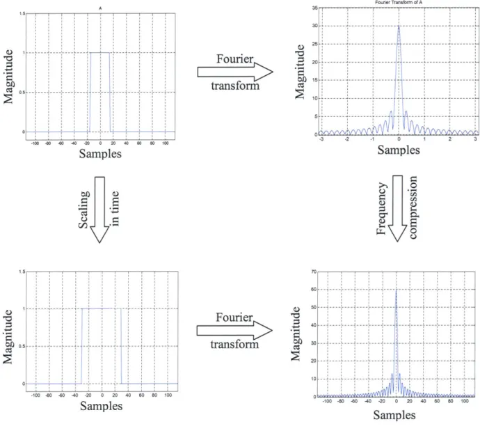
compression in frequency and increase of the magnitude of the frequency components. This property holds also in the DFT case; however there are mathematic complications, discussed in detail in [Oppenheim, 1998], which are irrelevant to our project and will be left out. Figure 3.1 shows examples of Fourier transform properties.
One of the most useful properties of the Fourier transform, which also hold for the DFT, is its application to convolution. The convolution of two functions,
f,
[n] andf
2 [n] is defined by:g[n]=
f,
[n]*f 2 [n]=f
[k]f 2 [n -k. (3.17)If we now take the DFT of Equation 3.17 we obtain:
G (e") = F (e e'", (3.18)
which shows that using DFT we can simplify a convolution to a simple product. This property, combined with fast numerical methods, like FFT [Bose, 2004], for calculating the Fourier transforms is the basis of all modem signal and image processing.
In CT scanner applications we are also interested in two-dimensional Fourier transforms. The two-dimensional DFT of a function
f
[x,
y] is defined as:F(u,v)= f [x, y]e"(ux+y), (3.19)
y=-00 x=-00
and its inverse is defined as:
f [ x,4y = f F (u,v j e "''dudv . (3.20)
4; 2r 2)2
All properties of the one-dimensional Fourier transforms can be extended to the two
_- - -j--- - - - - -- --- -- --100 -80 -80 -40 -20 0 20 40 80 0 100 Samples 30 Fourier transform 25 ; 20 10 5 -A 0,5 0
H
~ II
.~ c~ 11-4-i oil ~ --- -- -- -- ---100 -80 -0 -40 -20 0 20 40 60 80 100 Samples Fourier transform CIS 60 40 30 20 10 -100 -80 -80 -40 -20 0 20 40 60 80 100 SamplesFigure 3.1: Basic Fourier transform properties.
3.2.
Fundamentals of X-ray Physics
3.2.1. Generation of X-rays
X-rays are a type of electromagnetic waves, similar to microwaves, infrared, visible, and ultraviolet light, and radio waves. The wavelength of the x ray ranges from a few pico-meters (1 pm = 10-2 m) to a few nanometers (1 nm = 10-9 m). The energy of each
x-ray photon, E, is proportional to its frequency, v, and is given by:
-3 -2 -1 0 1 2 3 Samples >1 Fourier Transform of A S--- - -- -- --- --- --- ---- - - --- - - - - --- -- - - --- -- - --- --- --- - -- ----- - --- --- --- - --- -- -- -- -~ 1 1 \ 1.5 0.5 A -- -- -- - -- -- -- - --- - --- ---- -- --- --- --- - ---I- -- - - - - - ----- -- -- - ---- -I-
--E=hv= hc, (3.21)
2
where h is the Plank's constant (h = 6.63 x 10- J s), c is the speed of light, and A is
the wavelength of the x-rays. It is clear from Equation 3.21 that x-ray photons with longer wavelengths have lower energies than the photons of shorter wavelengths.
For convenience, the x-ray energy is usually expressed in units of electron-volts (1 eV = 1.602x 10⁻¹⁹J). This is the amount of kinetic energy with which and electron is
accelerated across an electrical potential of 1 V. Because x-ray photons are generally produced by striking a target material with high-speed electrons (the kinetic energy is transformed into electromagnetic radiation), the maximum possible x-ray photon energy equals the entire kinetic energy of the electron. For convenience in calculations, Equation
3.21 can be converted into units of eV per nm:
E = .24xleVnm (3.22)
X-rays with wavelengths in the range of 10 nm (124 eV) to 0.1 nm (12.4 keV) are often called "soft" x-rays, because they lack the ability to penetrate thicker layers of materials. These x rays have little value in radiology. The wavelength of diagnostic x rays varies roughly from 0.1 nm to 0.01 nm, corresponding to an energy range of 12.4 keV to 124 keV. Although x-rays with much shorter wavelengths are highly penetrating, they provide little low-contrast information and therefore, are of little interest to diagnostic imaging.
It is worth pointing out that x rays are at the high-energy (short wavelength) end of the electromagnetic spectrum. Figure 3.2 shows the entire electromagnetic spectrum with different types of electromagnetic waves labeled.
X-ray photons are produced when a substance is bombarded with high-speed electrons. When a high-speed electron interacts with the target material, different types of collisions take place. The majority of the encounters involve small energy transfers from the high-speed electron to electrons that are knocked out of the atoms, leading to ionization of the target atoms. This type of interaction does not produce x-rays and gives
rise to delta rays and eventually heat. For a typical x-ray tube, over 99% of the input energy is converted into heat.
radio walves microwaves infrared radiaitior ultraviolet radiation X-rays gamma rays vsible Iight
Figure 3.2: Electromagnetic spectrum. [Image taken from Wikipedia, 20061
More interesting interactions occur when the electron approaches the nucleus of the atom and suffers a radiation loss. The high-speed electron travels partially around the nucleus due to the attraction between the positive nucleus and the negative electron. The sudden deceleration of the electron gives rise to the so-called bremsstrahlung radiation. The energy of the resulting radiation depends on the amount of incident kinetic energy that is given off during the interaction. If the energetic electron barely grazes the atomic coulomb field, the resulting x-rays have relatively low energy. As the amount of interaction increases, the resulting x-ray energy increases.
It is interesting to note that x-rays can also be produced by other charged particles, such as protons or alpha particles. The total intensity of the bremsstrahlung radiation, I, resulting from charged particle of mass m and charge z incident on target nuclei with charge Z, is proportional to:
S z 2Z4 e6 (3.23)
Given that an the mass of an electron in 2000 times less that that of a massive particle, an electron is more than 4x 10⁶ times more efficient in generating bremsstrahlung radiation than a massive particle such as a proton. This is why high-speed electrons are the practical choice for the production of x-rays. Equation 3.23 also
indicates that the bremsstrahlung radiation production efficiency increases rapidly as the atomic number of the target increases.
The second type of radiation generating interaction occurs when a high-speed electron collides with one of the inner-shell electrons of the target atom and liberates it. When the hole is filled by an electron from an outer shell, characteristic radiation is emitted. In the classic Bohr model of the atom, electrons occupy orbits with specific quantized energy levels. The energy of the characteristic x-ray is the difference between the binding energies of two shells. For example, the binding energies of the K, L, M, and
N shells of tungsten are 70 keV, 11 keV, 3 keV, and 0.5 keV, respectively. When a
K-shell electron is liberated and the hole is filled with an L-K-shell electron, a 59 keV x-ray photon is generated. Similarly, when an M-shell electron moves to the K-shell, the x-ray photon produced has 67 keV of energy. Note that each element in the periodic table has its own unique shell binding energies, and thus the energies of characteristic x-rays are unique to each atom.
Before concluding this section, we would like to point out the distinction between kV (electric potential) and keV (energy). The unit kVp is often used to describe an x-ray source. For instance, a 120 kVp x-ray source indicates that the applied electric potential across the x-ray tube is 120 kV. Under this condition, the electrons that strike the target have 120 keV of kinetic energy. The highest energy photons that can be produced by such a process have energy of 120 keV.
3.2.2. X-rays - Matter Interactions
The typical energy range of an x-ray photon generated in a medical CT scanner is between 20 keV and 140 keV. In this energy range there are three fundamental ways in which x-rays interact with matter: the photoelectric effect, the Compton effect, and coherent scattering.
We start with a description of the photoelectric effect. When the x-ray photon energy is greater than the binding energy of an electron, the incident x-ray photon gives up its entire energy and liberates an electron a shell of an atom. The free electron is called a photoelectron. The hole created at the deep shell is filled by and outer-shell electron. Because the outer shell electron is at higher energy state than the inner shell, a
characteristic radiation results. Thus, a photoelectron effect produces a positive ion, a photoelectron, and a photon of characteristic radiation. This effect was first explained by Albert Einstein in 1905, for which he received the Nobel Prize in Physics in 1921.
For tissue-like materials, the binding energy of the K-shell electrons is very small (roughly 500 eV). Hence, the photoelectron acquires essentially the entire energy of the x-ray photon. In addition, at such low energy, the characteristic x-rays produced in the interaction do not travel far, usually less than the dimensions of a human cell. Even for materials such as calcium (a bone constituent), the K-shell binding energy is only 4 keV. Because the mean free path of a 1 keV x-ray photon in muscle tissue is about 2.7 [tm, we can safely assume that all of the characteristic x-rays produced in patients by the photoelectric effect are reabsorbed.
The second type of interaction is the Compton effect, named after Arthur Holly Compton, who received the Nobel Prize in 1927 for its discovery. This is the most important interaction mechanism in tissuelike materials. In this interaction, the energy of the incident x-ray photon is considerably higher than the binding energy of the electron. An incident x-ray photon strikes and electron and frees the electron from the atom. The incident x-ray photon is deflected or scattered with partial loss of its initial energy. A Compton interaction produces a positive ion, a "recoil" electron, and a scattered photon. The scattered photon may be deflected at any angle from 0 deg to 180 deg. Low energy x-ray photons are preferentially backscattered (deflection angle larger than 90 deg), whereas high-energy photons have a higher probability of forward scattering (deflection angle smaller than 90 deg). Because of the wide deflection angle, the scattered photon provides little information about the location of interaction and the photon path.
Most of the energy is retained by the photon after a Compton interaction. The deflected photon may undergo additional collisions before exiting the patient. Because only a small portion of the photon energy is absorbed, the energy (or radiation dose) absorbed by the patient is considerably less than the photoelectric effect. The probability of a Compton interaction depends on the electron density of the material, not the atomic number Z. The lack of dependence on the atomic number provides little contrast information between different tissues (the electron density difference between different tissues is relatively small). Consequently, nearly all of the medical CT devices try to
minimize the impact of the Compton effect by either post-patient collimation or algorithmic correction.
The third type of interaction is the coherent scattering (also known as Rayleigh scattering). In this interaction, no energy is converted into kinetic energy, and ionization does not occur. The process is identical to what occurs in the transmitter of a radio station. The electromagnetic wave with an oscillating electric field sets the electrons in the atom into momentary vibration. These oscillating electrons emit radiation of the same wavelength. Because the scattering is a cooperative phenomenon, it is called coherent scatter.
Coherent scattering occurs mainly in the forward direction to produce a slightly broadened x-ray beam. Because no energy is transferred to kinetic energy, this process historically has limited interest to CT. Recent research, however, has shown that coherent scatter can be used for bone characterization [Westmore, 1997] and [Batchelar, 2000].
The net effect of these interactions is that some photons are absorbed, some are scattered, and some go through. In simple terms, x-ray photons are attenuated as they pass through matter. The attenuation can be expressed by an exponential relationship for a monochromatic incident x-ray beam and a material of uniform density and atomic number as:
I= Ie , (3.24)
where I and I0 are the incident and transmitted x-ray intensities, L is the material thickness, and p is the linear attenuation coefficient of that material. This is often referred to as the Lambert-Beers law.
3.2.3. Radiation Dose
Ionizing radiation can cause tissue damage in a number of ways. The largest risk is that of cancer arising from the genetic mutations caused by chromosomal aberration [Webb, 2003]. The effects of radiation can be both deterministic and stochastic. Deterministic effects, caused by high doses of radiation, are usually associated with cell death. These effects are characterized by a dose threshold, below which no cell death is
observed. In contrast, stochastic effects occur at low radiation doses and the amount of radiation is proportional to the probability of a cell mutation.
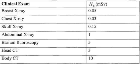
The absorbed dose D is equal to the radiation energy E absorbed per unit mass. D is usually measured in units of grays (Gy), where 1 Gy equals 1 J/kg. Many non-scientific publications measure the absorbed dose in rads, where 1 Gy is equal to 100 rads. In a medical environment, the patient dose is often specified in terms of the entrance skin dose, with typical values of 0.1 mGy for a chest radiograph and 1.5 mGy for an abdominal radiograph. Such measurements, however, give little indication of the risk to the patient. The most useful measure of radiation dose is the effective dose equivalent,
HE, which is the sum of the dose delivered to each organ weighted by the radiation sensitivity w of that organ with respect to cancer mutations:
HE = uwH 1 , (3.25)
where i is the number of organs irradiated and H, is the dose equivalent for each organ. The value of H is given by the absorbed dose D multiplied by the quality factor QF of
the radiation. Table 3.2 lists quality factors for different types of radiation.
Table 3.2: Quality factors of various types of ionizing radiation.
Radiation Type Quality Factor
x-rays 1
-y-rays 1
neutrons 10
a-particles 20
Both H and HE are measured in sieverts (Sv). Older literature measures the dose equivalent and the effective dose equivalent in units of rems, where 1 Sv equals 100 rems. Typical values of the radiation sensitivity of different organs, used for the calculation of HE, are given in Table 3.3.
In CT applications the radiation dose to the patient is calculated in a slightly different manner because the x-ray beam profile across each slice is not uniform and adjacent
slices receive some dose from one another. The Unites States Food and Drug Administration (FDA) defines the Computed Tomography Dose Index (CTDI) for a 14-slice exam to be:
CTDI= TDdz, (3.26)
where Dz is the absorbed dose at position z and T is the thickness of each slice. Still, in terms of addressing patient risk the value of HE is a better measure. Table 3.4 lists typical values of HE associated with standard clinical exams. The limit in annual radiation dose under federal law in the United States is 0.05Sv (5000 mrem) and corresponds to over 1000 planar chest x-rays, 15 head CTs, or 5 full-body CTs
Table 3.3: Radiation sensitivity of various organs.
Organ Radiation Sensitivity
Gonads 0.2 Lung 0.12 Breast 0.1 Stomach 0.12 Skin 0.01 Thyroid 0.05
Table 3.4: Effective Dose Equivalent HE for Clinical X-ray and CT Exams
Clinical Exam HE (mSv) Breast X-ray 0.05 Chest X-ray 0.03 Skull X-ray 0.15 Abdominal X-ray 1 Barium fluoroscopy 5 Head CT 3 Body CT 10
4. Image Processing
4.1.
Image Reconstruction
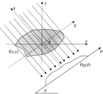
In this section we will deal with the mathematical basis of computed tomography with non-diffracting sources. We will show how one can go about recovering an image of the cross section of an object from projection data.
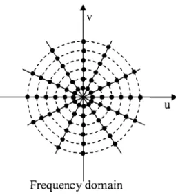
This chapter will start with the definition of line integrals and how they are combined to form projections of an object. By finding the Fourier transform of a projection taken along parallel lines, we will then derive the Fourier Slice Theorem. We will also discuss reconstruction algorithms based on parallel beam projection data and fan beam projection
data.
4.1.1. Line Integral Measurements
In Chapter 2 we learned that computed tomography relies on x-ray flux measurements from different angles to form an image. At each angle, the measurement is essentially identical to that of the conventional x-ray radiography. We record the x-ray flux impinging on the x-ray detector after attenuation by an object. If we assume that the input x-ray photons are monoenergetic, the x-ray intensities measured on the entrance and the exit slides of a uniform material, shown in Figure 4.1 (a), follow the Lambert-Beers law [Herman, 1980], as discussed in Section 3.2.2.
I = Ioe-", (4.1)
In this equation, I0 is the entrance x-ray intensity, I is the exit x-ray intensity, Ax is the thickness, and p is the linear attenuation coefficient of the material. In general, u changes with the x-ray energy and varies with the type of material.
/10
>
L
eL>
/A
P~2 P3 P14 P,=0 =
a) b)
Figure 4.1: Monochromatic x-ray attenuation. a) Attenuation by an uniform object
b) Attenuation by a non-uniform object
From Equation 4.1, it is clear that objects with higher p values are more attenuating to x-ray photons than objects with lower p values. For example, the p value of bones is higher than that of soft tissues, indicating the fact that it is more difficult for x-ray photons to penetrate bones than soft tissues. On the other hand, the p value for air is nearly zero, indicating the fact that the input and output x-ray flux is virtually unchanged
by passage through air.
Let us now consider the case of a non-uniform object. The overall attenuation characteristics can be calculated by dividing the object into small elements, as shown in Figure 4.1b. When the size of the elements is sufficiently small, each element can be considered as a uniform object. Equation 4.1 can be used to describe the entrance and exit x-ray intensities for each element. Observing the fact that the exit x-ray flux from an element is the entrance x-ray flux to its neighbor, Equation 4.1 can be applied repeatedly in cascade fashion. Mathematically, the exiting intensity can be expressed as:
I= I0e-4 xe-yAxe-AxK e-nAX = 10e "= . (4.2)
If we divide both sides of Equation 3.2 by lo and take the negative logarithm of the
P = -ln -= iAx. (4.3)
As Ax approaches zero, the summation changes into an integral over the entire object and Equation 4.3 becomes:
p=-inK j= fu(x)dx. (4.4)
In CT scanner applications, p is the projection measurement. Equation 4.4 states that the ratio of the input x-ray intensity over the output x-ray intensity, after logarithm operation, represents the line integral of the attenuation coefficient along the x-ray path. The reconstruction problem for CT can now be stated as the following: given the measured line integrals of an object, how do we estimate or calculate its attenuation coefficients?
4.1.2. Algebraic Reconstruction Technique
To understand some of the methods employed in the CT reconstruction, let us begin with an extremely simplified case in which the object is formed with four small blocks. The attenuation coefficients are homogeneous within each block and are labeled it,, /12,
14, and pt4, as shown in Figure 4.2. Let us further consider the scenario where line
integrals are measured along the horizontal, vertical, and diagonal directions. Five measurements in total are selected in this example. It can be shown that the diagonal and three other measurements form a set of independent equations. For example
p = AJ + p2
P2 = P3 + P4 (4.5)
P = A + pU3 P4 = A+ P4
Four independent equations are established for the four unknowns. From elementary algebra we know that there is a unique solution to the problem, as long as the number of equations equals the number of unknowns. If we generalize this to the case where the object is divided into N by N small elements, we could easily reach the conclusion that as