Reconfigurable transmitarrays for beam-steering and beam -forming at millimeter-waves

(1)

HAL Id: tel-02183145

https://tel.archives-ouvertes.fr/tel-02183145

Submitted on 15 Jul 2019

HAL is a multi-disciplinary open access

archive for the deposit and dissemination of sci-entific research documents, whether they are pub-lished or not. The documents may come from teaching and research institutions in France or abroad, or from public or private research centers.

L’archive ouverte pluridisciplinaire HAL, est destinée au dépôt et à la diffusion de documents scientifiques de niveau recherche, publiés ou non, émanant des établissements d’enseignement et de recherche français ou étrangers, des laboratoires publics ou privés.

beam -forming at millimeter-waves

Fatimata Diaby

To cite this version:

Fatimata Diaby. Reconfigurable transmitarrays for beam-steering and beam -forming at millimeter-waves. Optics / Photonic. Université Grenoble Alpes, 2018. English. �NNT : 2018GREAT125�. �tel-02183145�

(2)

Pour obtenir le grade de

DOCTEUR DE LA

COMMUNAUTÉ UNIVERSITÉ GRENOBLE ALPES

Spécialité : OPTIQUE ET RADIOFREQUENCES

Arrêté ministériel : 25 mai 2016

Présentée par

Fatimata DIABY

Thèse dirigée par Laurent DUSSOPT , Ingénieur chercheur, CEA préparée au sein du Laboratoire CEA/LETI

dans l'École Doctorale Electronique, Electrotechnique,

Automatique, Traitement du Signal (EEATS)

Réseaux transmetteurs reconfigurables pour

le dépointage et la formation de faisceau en

bande millimétrique.

Reconfigurable transmitarrays for

beam-steering and beam -forming at

millimeter-waves.

Thèse soutenue publiquement le 14 décembre 2018, devant le jury composé de :

Monsieur LAURENT DUSSOPT

INGENIEUR DE RECHERCHE, CEA GRENOBLE, Directeur de thèse

Madame CLAIRE MIGLIACCIO

PROFESSEUR, UNIVERSITE NICESOPHIA- ANTIPOLIS, Rapporteur

Monsieur SYLVAIN BOLIOLI

INGENIEUR, ONERA CENTRE MIDI-PYRENEES, Rapporteur

Madame PAOLA PIRINOLI

PROFESSEUR, UNIVERSITE POLYTECHNIQUE TURIN - ITALIE, Examinateur

Monsieur HERVE AUBERT

PROFESSEUR, INSTITUT NATIONAL POLYTECHNIQUE TOULOUSE, Président

Monsieur RONAN SAULEAU

PROFESSEUR, UNIVERSITE RENNES 1, Examinateur

Monsieur LAURENT PETIT

INGENIEUR DE RECHERCHE, RADIALL CENTR'ALP VOREPPE, Examinateur

Monsieur ANTONIO CLEMENTE

(3)

(4)

i

I would like to also address my thankful to my supervisor Dr. Antonio Clemente, Research Engineer at CEA-Leti. Throughout this work, he has provided me constant support, great availability and listening. Thanks for your constructive criticism and advices which are guided me throughout this thesis. I am aware of having benefited from high quality scientific supervision.

I am also very thankful to Prof. Ronan Sauleau, Professor at the University of Rennes for your precious comments and suggestions which have guided this work to the end. I would like to express my gratitude to having accepted to be a part of the jury.

I would like to address my acknowledgment to Dr. Christophe Delaveaud (Head of Laboratory Antenna, Propagation and Inductive Coupling), Fabien Clermidy (head of Wireless Technologies Services), and Sébastien Dauve (head of the Department DSYS), for welcoming me during the three years of this thesis, for allowing me to work in very good conditions and putting at my disposal all the means necessary for the smooth running of my thesis.

I acknowledge the members of my thesis jury for having accepted to examine this thesis, Prof. Claire Migliaccio, Dr. Sylvain Bolioli, Prof. Paola Pirinoli, Prof Hervé Aubert, and Dr. Laurent Petit.

I would also like to thank all the members of the LAPCI for their availability and sympathy.

Finally, I could not finish these thanks without thinking of my family whose affection, constant love, support and encouragement have been a great comfort to me and have contributed to the completion of this work.

(7)

iv

List of Tables

Table I-1: IEEE radar-frequency letter band definition. ... 5

Table I-2: Antenna main specifications for automotive radars. ... 7

Table I.3: Key system parameters of the mm-wave beamforming prototypes [13]. ... 9

Table I.4: Impact of phase quantization on the TA performances. ... 28

Table I.5: Performances of existing fixed beam transmitarrays. ... 52

Table I.6: Performances of existing switched beam transmitarrays. ... 53

Table I.7: Performances of existing electronically beam transmitarrays. ... 54

Table II-1: Impact of phase quantization on the TA performances. ... 60

Table II-2: Performance of the TA when the beam points at 30°. ... 62

Table II-3: Performance of the TA when the beam points at 60°. ... 62

Table II-4: Maximum gain of the 3-facet TA as function of the desired scan angle. ... 68

Table II-5: Maximum gain of the 3-facet TA as a function of the desired scan angle: config. 1 (30×20 elements). ... 72

Table II-6: Maximum gain of the 3-facet TA as a function of the desired scan angle: config. 2 (40×40 elements). ... 72

Table II-7: Maximum gain of the 3-facet TA as a function of the desired scan angle: config 3 (50×20 elements). ... 73

Table III-1: Main features of the 1-bit simple patch unit-cell. ... 77

Table III-2: Performance of the proposed linearly-polarized transmitarray at 29 GHz. ... 86

Table III-3: Geometrical dimensions of the proposed unit-cell. ... 89

Table III-4: Effect of phase quantization on the 1600-element circularly-polarized transmitarray. ... 93

Table III-5: Measured performances of the proposed 1600-element fixed-beam transmitarray ... 98

Table IV-1: Dimensions of the proposed 2-bit unit-cell (Figure IV-1(a)). ... 109

Table IV-2: Different combinations of the reception and transmission layers corresponding to the four phase states. ... 109

Table IV-3: Simulated performances of the 2-bit linearly-polarized unit-cell. ... 110

Table IV-4: Measured and simulated performances in the waveguide of the 2-bit linearly-polarized unit-cell. ... 118

Table IV-5: Simulated performances of the 2-bit circularly-polarized unit-cell... 124

Table IV-6: Summary of the 2-bit circularly-polarized unit-cell performances. ... 127

Table V-1: Summary of the 2-bit electronically reconfigurable transmitarray performances in E plane at 29 GHz. ... 141

Table V-2: Summary of the 2-bit electronically reconfigurable transmitarray performances in H plane at 29GHz. ... 142

Table V-3: Summary of the 2-bit electronically reconfigurable transmitarray performances at broadside (Measurement, theoretical results with and without errors). ... 145

(8)

(9)

vi

List of Figures

Figure 1 : Réseau transmetteur à 3 facettes : (a) vue schématique, (b) diagrammes de

rayonnement (simulé et théorique) à 29 GHz sur le plan E. ... xvii Figure 2 : Réseau transmetteur à faisceau collimaté : (a) gain et (b) rapport axial en fonction de la fréquence. ... xviii Figure 3 : Diagrammes de rayonnement (polarisation circulaire gauche) simulés et mesurés du réseau transmetteur à quatre faisceaux dans les (a) plan horizontal (29 GHz) et plan vertical (29 GHz). ... xix Figure 4 : Diagrammes de rayonnement mesurés du réseau transmetteur électroniquement reconfigurable dans les plans E (a) et H (b) à 29 GHz) en fonction de l'angle de l’angle de dépointage de ± 60 °. ... xx Figure I-1: D-RAN and C-RAN 5G network architectures with backhaul and fronthaul [9]. ... 8 Figure I-2: Configuration of the mm-wave beamforming prototype [13]. ... 9 Figure I-3: 28 GHz phased array transceiver. (a) Measurement setup. (b) E plane radiation pattern at 29.5 GHz. ... 10 Figure I-4: Single layer polarization independent reflectarray antenna. (a) Top view of the unit-cell. (b) Radiation patterns in E-plane. ... 10 Figure I-5: (a) 3-D view and (b) radiation patterns in E-plane of the proposed folded

reflectarray antenna at 38 GHz. ... 11 Figure I-6: Measured normalized radiation patterns in E-, and H-plane at 60 GHz with ETSI masks: (a) polarization in x-direction, (b) polarization in y-direction. ... 11 Figure I-7: Co-polar (solid line) and cross-polar (dotted line) components radiation masks of the ETSI 302 217 in the frequency band (a) 24 – 30 GHz, and (b) 30 – 47 GHz. ... 12 Figure I-8: Alternative radiation masks of the Class 3 antenna defined by of the ETSI 302 217 in the frequency band 30 – 47 GHz. (a) Class 3B and (b) class 3C. ... 12 Figure I-9: The main building blocks of a satellite communication system. ... 13 Figure I-10: ThinKom’s agile, ThinAir® Falcon-Ka2517 antenna for broadband air flight connectivity [19]. ... 14 Figure I-11: 70cm Ku-band MSAT beam patterns vs. scan angle [20]. ... 14 Figure I-12: (a) 51 cm diameter Ku-band Variable Inclination Continuous Transverse Stub (VICTS) array. (b) Measured elevation-plane pattern for the 51 cm VICTS array at 12.5 GHz (scanned to 63 degrees) [21]. ... 15 Figure I-13: Prototype of an 8x8-element aperture (1) and two stacked waveguide networks for horizontal (2) and vertical polarization (3) for achieving arbitrary polarization control, and broadside radiation patterns. ... 15 Figure I-14: X/Ka Commander Integrated Antenna/Terminal Subsystem. ... 16 Figure I-15: K/Ka band array antenna for Office-in-the-Air Connectivity. ... 16 Figure I-16: Simulated and measured directivity patterns of the FSS-backed reflectarray antenna in transverse plane at 20 GHz (left) and 29.8 GHz (right)... 17

(10)

vii Figure I-17: Prototype of the proposed Ka-band reflectarray antenna integrated with solar cells (left) and measured gain within the operating frequency band (right). ... 17 Figure I-18: 3-D view of the folded reflectarray antenna for SatCom applications at Ka-band (left), and radiation patterns (calculated and measured) at 60° in ϕ = 0° cut plane (right). ... 18 Figure I-19: Reflectarray prototype (left), and measured versus simulated gain in Ku/Ka bands for H-polarization (right). ... 19 Figure I-20: Frequency band allocations for SatCom applications according to ITU. ... 20 Figure I-21: Ka-band SatCom coverage. (a) Ka-Sat coverage [31]. (b) Launch of satellites offering lower cost per bit Ku/Ka-bands capability [32]. (c) Satellite interface in Inmarsat Global Xpress [33], (d) Terminal characteristics for Inmarsat Global Xpress [33]. ... 21 Figure I-22: Power mask of recommendations ETSI EN 301 360 and ETSI EN 301 459 in the case of one Earth Terminal. ... 22 Figure I-23: Radiation mask of recommendation ITU S.465-6. ... 22 Figure I-24: Power mask of recommendation FCC 25.138. The masks are calculated

considering one earth terminal (TDMA carriers with bandwidth > 40 kHz). ... 22 Figure I-25: Power mask of recommendation ETSI EN 303 978. The masks are calculated considering one Earth Terminal (TDMA carriers with bandwidth > 40 kHz). ... 23 Figure I-26: (a) Schematic view of a transmitarray antenna. (b) Full power budget of a TA. 24 Figure I-27: Full-wave electromagnetic simulation setup of a unit-cell using periodic

boundary conditions and Floquet port excitation. ... 25 Figure I-28: (a) Prototype of the proposed bidrectional high gain array. (b) Simulated and measured transmitted (TA) and reflected (RA) gains of the Bi-HGA versus frequency [54]. 29 Figure I-29: High-efficiency wideband transmitarray antenna. (a) Fabricated prototype, (b) measured and simulated realized gain and aperture efficiency of the proposed transmitarray antenna. ... 29 Figure I-30: Simulated and measured co- and cross-polar radiation patterns in E-plane (a) 11 GHz, and (b) 12.5 GHz. ... 30 Figure I-31: (a) Fabricated wideband transmitarray under measurement. (b) Measured and simulated gains as a function of frequency [57]... 31 Figure I-32: 20 GHz double-layer linearly-polarized transmitarray antenna using Malta crosses with vias [58]. ... 31 Figure I-33: Circularly-polarized transmitarray with sequential rotation at 30 GHz [41]. (a) 3-D exploded view of the unit-cell. (b) Simulated and measured radiation patterns in horizontal plane. ... 32 Figure I-34: Ultra low profile transmitarray using multifolded ray tracing principle [59]. (a) 3-D exploded view of the unit-cell. (b) Simulated and measured radiations patterns. ... 33 Figure I-35: Circularly-polarized transmitarray based on linearly-polarized unit-cell [60]. (a) Architecture of the unit-cell. (b) Axial ratio as a function of frequency. ... 33 Figure I-36: Dual-band circularly-polarized transmitarray for SOTM systems [61]. (a)

Perspective view of the unit-cell. (b) Broadside radiation pattern at 20 GHz and 30 GHz. .... 34 Figure I-37: Dual-band transmitarray at Ka-band with the capability of forming independent linearly-polarized beams [62]. (a) Beam directions of the proposed prototypes. Theoretical and measured gain as a function of frequency in (b) up link and (c) down link bands... 35 Figure I-38: (a) Phase delay (PD) unit-cell. (b) Phase rotation (PR) unit-cell. Performances of both TA types [63]. ... 36 Figure I-39: 60 GHz linearly-polarized transmitarray for backhauling [64]. (a) Prototype of the TA. (b) Measured and simulated gain as a function of frequency. (c) Co-, and

(11)

cross-viii polarization radiation patterns of the TA for different frequencies (57 GHz, 61.5 GHz, and 66 GHz) compared to ETSI masks. ... 37 Figure I-40: Fabricated 140 GHz high gain LTCC-integrated transmitarray (left); simulated and measured gain and corresponding efficiency within the frequency band of interest (right) [65]. ... 37 Figure I-41: Prototype and frequency response (gain as a function of frequency) of the two-layer transmitarray [66]. ... 38 Figure I-42: High-gain dual band-beam steering transmitarray at Ka-band. (a) Unit-cell configuration. Measured radiation patterns at (b) 20 GHz and (c) 30 GHz [67]. ... 39 Figure I-43: Prototype of the proposed lens with seven-element feeding antenna (left), and measured scanned beam at 28 GHz (right) [68]. ... 39 Figure I-44: Switched-beam transmitarray at V-band [69]. (a) Principle. (b) Experimental radiation patterns in H-plane at 61 GHz. ... 40 Figure I-45: Coplanar transmitarray with four SIW slot primary feeds at 76.5GHz [70]. ... 40 Figure I-46: 36-element reconfigurable transmitarray based on varactors at 5 GHz [71]. (a) Unit cell design. (b) Prototype of the TA. Measured radiation patterns (c) E-plane, (d) H-plane. ... 42 Figure I-47: Reconfigurable transmitarray with beam-steering and polarization conversion capabilities [72]. (a) Architecture of the proposed unit-cell. (b) Far-field radiation patterns in E-plane at 5.4 GHz. ... 43 Figure I-48: Circularly-polarized reconfigurable transmitarray antenna [73]: (a) architecture of the unit-cell, (b) far-field radiation pattern in the diagonal plane at 4.8 GHz. ... 43 Figure I-49: Electronically-reconfigurable transmitarray with integrated leaky-wave feed [74]. (a) Exploded model of the proposed TA. (b) Measured and simulated co-polarized realized gain at 4.8 GHz in the diagonal plane. ... 44 Figure I-50: Measured radiation patterns at 5.2 GHz for different steering angles in azimuth (left) and elevation (right) planes [75]. ... 44 Figure I-51: (a) Schematic model of the amplifying unit-cell with electronically reflection-type phase shifter. Measured frequency responses: (b) transmission coefficient, (c) phase tuning range [76]. ... 45 Figure I-52: Electronically reconfigurable transmitarray in X-band [77]. (a) Schematic view of the TA. (b) H-plane beam scanning capability. ... 45 Figure I-53: Electronically reconfigurable circularly-polarized transmitarray in X-band [78]. (a) Schematic view of the unit-cell. (b) Measured transmission characteristics of the fabricated transmitarray. ... 46 Figure I-54: Dual linearly polarized unit-cell with 1-bit phase resolution in X-band [79]. ... 47 Figure I-55: Circularly-polarized reconfigurable transmitarray unit cell based on microfluidics at X band [80]. ... 47 Figure I-56: A Ku-band 1-bit reconfigurable transmitarray: architecture of the proposed unit-cell (left), and radiation patterns (right) [81]. ... 48 Figure I-57: K-band linearly-polarized reconfigurable transmitarray: fabricated prototype (left), and radiations patterns (right) [82]. ... 48 Figure I-58: 2-bit electronically reconfigurable transmitarray based on RF-MEMS switched unit-cells [84]. ... 49 Figure I-59: (a) Prototype of a Ka-band 400-element circularly polarized transmitarray, (b) simulated and measured frequency response (broadside) [85]. ... 49

(12)

ix Figure I-60: (a) Active dual-band TA and realized module. Measured and simulated radiation patterns: (b) Receive antenna at 20 GHz, (c) Transmit antenna at 30 GHz [86]. ... 50 Figure II-1: TA peak gain at broadside for three different TAs and for both phase

compensation techniques as a function of the normalized frequency f/f0. ... 59

Figure II-2: Phase distribution of the 40×40 TA when TTD phase compensation technique is used for the normalized frequencies f/f0. ... 59

Figure II-3: (a) Radiation patterns (E-plane) of the 40×40 TA for three different frequencies using constant phase-shift compensation, (b) A zoom on the main beam for elevation angle 0

ranging from -10° to 10°. ... 60 Figure II-4: (a) Radiation patterns (E-plane) of the 40×40 TA for three different frequencies using true-time delay compensation, (b) A zoom on the beam for elevation angle 0 ranging

from -10° to 10°. ... 60 Figure II-5: Radiation patterns of the 40×40 TA steered at 30° in E-plane. (a) Constant phase-shift compensation. (b) TTD compensation. ... 61 Figure II-6: (a) Radiation patterns of the 40×40 TA steered at 60° in E-plane. (a) Constant phase-shift compensation. (b) TTD compensation... 61 Figure II-7: (a) Radiation patterns (E-plane) of the 40×40 TA for three different frequencies using constant phase-shift compensation when the beam is steered at 60°, (b) zoom on the beam for elevation angle 0 ranging from 50° to 70°. ... 63

Figure II-8: (a) Radiation patterns (E-plane) of the 40×40 TA for three different frequencies using TTD compensation when the beam is steered at 60°, (b) zoom on the beam for elevation angle 0 ranging from 50° to 70°. ... 63

Figure II-9: Three elementary rotations. (a) Around z-axis. (b) Around y-axis. (c) Around x-axis. ... 64 Figure II-10: Different shapes of transmitarray. (a) Flat shape. (b) 2-facets. (c) 3-facets. ... 65 Figure II-11: Schematic view of a 3-facet TA (left) and unit-cells used for full-wave

simulations (right). ... 66 Figure II-12: Normalized gain versus frequency of the 3-facet TA; comparison of the

theoretical model with a full-wave simulation. ... 67 Figure II-13: : Normalized gain versus frequency of the planar and 3-facet TAs. ... 67 Figure II-14: Schematic view of the 3-facet TAs for the three configurations : (a) config. 1 (30×20), (b) config. 2 (40×20), and (c) config. 3 (50×20). ... 69 Figure II-15: Gain versus focal ratio for the three configurations of the 3-facet TAs. ... 69 Figure II-16: (a) Radiation patterns of the three configurations of the 3-facet TA when the lateral panels are tilted at α = 0° (i.e. case of a planar array), (b) zoom on the beam for

elevation angle 0 ranging from 70° to 88°. ... 70

Figure II-17: (a) Radiation patterns of the three configurations of the 3-facet TA when the lateral panels are tilted at α = 10°, (b) zoom on the beam for elevation angle 0 ranging from

70° to 88°. ... 70 Figure II-18: (a) Radiation patterns of the thee configurations of the 3-facet TA when the lateral panels are tilted at α = 30°, (b) zoom on the beam for elevation angle 0 ranging from

70° to 88°. ... 70 Figure II-19: (a) Radiation patterns of the three configurations of the 3-facet TA when the lateral panels are tilted at α = 70°, (b) zoom on the beam for elevation angle 0 ranging from

70° to 88°. ... 71 Figure II-20: Phase distribution of the 3-facet TA with α = 70° in the config. 1 (5×20, 20×20, 5×20 panels). The beam is steered at 0 = 80°. ... 71

(13)

x Figure II-21: Phase distribution of the 3-facet TA with α = 70° in the config. 2 (10×20, 20×20, 10×20 panels). The beam is steered at 0 = 80°. ... 71

Figure II-22: Phase distribution of the 3-facet TA with α = 70° in the config. 3 (15×20, 20×20, 15×20 panels). The beam is steered at 0 = 80°. ... 72

Figure III-1: Proposed simple patch unit-cell with 1-bit phase resolution. (a) 3-D exploded view. (b) Top view. ... 77 Figure III-2: Simulated results of the simple patch unit-cell. (a) and (b) Magnitude of the reflection S11 and transmission S21 coefficients. (c) Transmission phase. (d) Differential

phase-shift. ... 78 Figure III-3: Impact of typical fabrication errors for the patch width on the S-parameters. (a) Reflection, (b) transmission coefficients. ... 79 Figure III-4: Impact of typical fabrication errors for the patch length on the S-parameters. (a) Reflection, and (b) transmission coefficients. ... 79 Figure III-5: Impact of the feed location on the S-parameters. (a) Reflection, and (b)

transmission coefficients. ... 80 Figure III-6: Impact of the ground-plane hole diameter on the S-parameters. (a) Reflection, and (b) transmission coefficients. ... 80 Figure III-7: Broadband unit-cell based on simple patches. (a) Top view. (b) Parameters values. ... 81 Figure III-8: Simulated S-parameters of the broadband unit-cell based on simple patch

antennas. Magnitude of the (a) reflection S11 and (b) transmission S21 coefficients. ... 82

Figure III-9: (a) Top view and (b) main features of the proposed U-shaped slot unit-cell. ... 82 Figure III-10: Simulated S-parameters of the U-shaped slot unit-cell. Magnitude of the (a) reflection S11 and (b) transmission S21 coefficients. ... 82

Figure III-11: (a) Top view and (b) main features of the proposed O-shaped slot unit-cell. ... 83 Figure III-12: Simulated S-parameters of the O-shaped slot unit-cell. Magnitude of the (a) reflection S11 and (b) transmission S21 coefficients. ... 83

Figure III-13: a) Top view and (b) main features of the proposed capacitively-coupled unit-cell ... 84 Figure III-14: Simulated S-parameters of the capacitively-coupled unit-cell. Magnitude of the (a) reflection S11 and (b) transmission S21 coefficients. ... 84

Figure III-15: Scheme of the eight unit-cells with 3 bits of phase quantization (top view). .... 85 Figure III-16: S-parameters of the 0°, 45°, 90°, 135°, 180°, 225°, 270° and 315° unit-cells. Magnitude of the (a) reflection S11, and (b) transmission S21 coefficients. (c) Transmission

phase. (d) Phase-shift between the 0° unit-cell and the other states. ... 85 Figure III-17: 20×20-element transmitarray with 3 bits of phase quantization. (a) Schematic view and phase distribution. (b) Gain as a function of frequency. ... 87 Figure III-18: Theoretical and full-wave simulated radiation patterns at 29 GHz in E-plane: (a) co-, (b) cross-polarizations. ... 87 Figure III-19: Theoretical and full-wave simulated radiation patterns at 29 GHz in H-plane: (a) Co-, (b) Cross-polarizations. ... 87 Figure III-20: Proposed 3-bit circularly-polarized unit-cell. (a) 3-D exploded view. (b)

Transmitting and receiving layers. ... 88 Figure III-21: S-parameters of 3-bit circularly-polarized unit-cells. Magnitude of the (a) reflection coefficients referred to the (a) receiving (S11) and (b) transmitting (S22) layers. (c)

(14)

xi Figure III-22: (a) Transmission phase and (b) phase-shift between the 0° unit-cell and the other states. ... 90 Figure III-23: Theoretical and simulated frequency responses of the 20×20-element circularly-polarized transmitarray: (a) broadside gain, and (b) axial ratio. ... 91 Figure III-24: 20×20-element circularly-polarized transmitarray: LHCP and RHCP radiation patterns in the 0° plane. ... 92 Figure III-25: 20×20-element circularly-polarized transmitarray: LHCP and RHCP radiation patterns in the 90° plane. ... 92 Figure III-26: Phase distribution of the 1-, 2-, and 3-bit transmitarray for a broadside beam. 93 Figure III-27: (a) Theoretical broadside gain, (b) and axial ratio as a function of frequency for the 3 transmitarrays. ... 94 Figure III-28: Comparison between the (a) co-, and (b) cross polarization radiation patterns of the 1-, 2-, 3-bit transmitarray and the ETSI masks. ... 94 Figure III-29: Theoretical and simulated radiation patterns in the 0° plane at 29 GHz: (a) LHCP, (b) RHCP. ... 94 Figure III-30: Theoretical and simulated radiation patterns in the 90° plane at 29 GHz: (a) LHCP, (b) RHCP. ... 95 Figure III-31: Circularly-polarized quad-beam transmitarray: (a) 3-D scheme, (b) 3-bit phase distribution optimized at 29 GHz. ... 95 Figure III-32: Theoretical and simulated LHCP and RHCP radiation patterns of the proposed quad-beam transmitarray in (a) vertical and (b) horizontal planes. ... 96 Figure III-33: Far-field measurement setup of the 1600-element single-beam circularly-polarized TA in (a) vertical and (b) diagonal planes. ... 97 Figure III-34: Theoretical and simulated frequency responses of the 1600-element single-beam circularly-polarized transmitarray: (a) broadside gain and (b) axial ratio. ... 97 Figure III-35: Simulated and measured radiation patterns of the 1600-element single-beam circularly-polarized transmitarray antenna: (a) vertical and (b) horizontal planes. ... 98 Figure III-36: Measured gain as a function of the frequency and elevation angle in the vertical plane: (a) LHCP, (b) RHCP. ... 99 Figure III-37: Measured radiation patterns (LHCP and RHCP) in the vertical, diagonal and horizontal planes at 27 GHz. ... 99 Figure III-38: Measured radiation patterns (LHCP and RHCP) in the vertical, diagonal and horizontal planes at 29 GHz. ... 99 Figure III-39: Measured radiation patterns (LHCP and RHCP) in the vertical, diagonal and horizontal planes at 32 GHz. ... 100 Figure III-40: Far-field measurement setup of the 489-element quad-beam transmitarray: (a) vertical, and horizontal planes. ... 100 Figure III-41: Theoretical, simulated, and measured frequency responses of the quad-beam transmitarray. ... 101 Figure III-42: Simulated and measured radiation patterns in the vertical plane at 29 GHz: (a) LHCP, (b) RHCP. ... 101 Figure III-43: Simulated and measured radiation patterns in the horizontal plane at 29 GHz: (a) LHCP, (b) RHCP ... 101 Figure III-44: Measured gain as a function of the frequency and elevation angle in the vertical plane. ... 102 Figure III-45: Measured gain as a function of the frequency and elevation angle in the

(15)

xii Figure IV-1: Proposed 2-bit linearly-polarized unit-cell: (a) Schematic view, (b) transmitting layer, (c) biasing layer of the transmission side, (d) DC connection to the ground layer, (e) ground plane, (f) biasing layer of the receive side, and (g) receiving layer. ... 107 Figure IV-2: Equivalent lumped-element models of the PIN diode (MA4GFCP907) in the

ON, and OFF states. ... 108

Figure IV-3: Surface current distribution: (a) and (b) on Tx layer, (c) and (d) on Rx layer. . 108 Figure IV-4: Frequency responses of the proposed 2-bit linearly-polarized unit-cell.

Magnitude of the (a) reflection and (b) transmission coefficients. (c) Transmission phase. (d) Phase-shift between the 0° state and the other states. ... 110 Figure IV-5: Bias lines arrangement of the 2-bit unit-cell: (a) transmitting Tx, (b) Tx biasing network, (c), receiving Rx, and (d) Rx biasing network layers. ... 111 Figure IV-6: Impact of bias lines on the performances of the proposed 2-bit linearly-polarized unit-cell: (a) 0°, (b) 90°, (c) 180°, and (d) 270° states. ... 112 Figure IV-7: Scheme of the waveguide setup to test the unit-cell. ... 112 Figure IV-8: Scattering-parameters of the 2-bit linearly-polarized unit-cell performed with a waveguide simulator and Floquet ports under oblique incidence : (a) 0°, (b) 90°, (c) 180°, and (d) 270° states. ... 114 Figure IV-9: (a) Transmission phase and (b) phase-shift between the 0° state and the other states performed in waveguide simulator. ... 114 Figure IV-10: Prototype of the proposed 2-bit linearly-polarized unit-cells: transmitting, and receiving layers on left and right, respectively. ... 115 Figure IV-11: Fabricated unit-cells with (a) bias wires and (b) placed in the waveguide. .... 115 Figure IV-12: Measured (in WR-28 waveguide) and simulated scattering parameters

magnitudes in the 0° state: (a) reflection (S11) and (b) transmission (S21) coefficients. ... 116 Figure IV-13: Measured (in WR-28 waveguide) and simulated scattering parameters

magnitudes in the 90° state: (a) reflection (S11) and (b) transmission (S21) coefficients. .... 116 Figure IV-14: Measured (in WR-28 waveguide) and simulated scattering parameters

magnitudes in the 180° state: (a) reflection (S11) and (b) transmission (S21) coefficients. .. 116 Figure IV-15: Measured (in WR-28 waveguide) and simulated scattering parameters

magnitudes in the 270° state: (a) reflection (S11) and (b) transmission (S21) coefficients. .... 117

Figure IV-16: (a) Measured transmission phase of the four states of the proposed 2-bit unit-cell and (b) phase-shift between the 0° state and the other states. ... 118 Figure IV-17: Impact of bias lines on the measured scattering parameters magnitudes in the waveguide in the 0° state: (a) reflection (S11) and (b) transmission (S21) coefficients. ... 119

Figure IV-18 Impact of bias lines on the measured scattering parameters magnitudes in the waveguide in the 90° state: (a) reflection (S11) and (b) transmission (S21) coefficients. ... 119

Figure IV-19: Impact of bias lines on the measured scattering parameters magnitudes in the waveguide in the 180° state: (a) reflection (S11) and (b) transmission (S21) coefficients. ... 119

Figure IV-20: Impact of bias lines on the measured scattering parameters magnitudes in the waveguide in the 270° state: (a) reflection (S11) and (b) transmission (S21) coefficients. ... 119

Figure IV-21: Holes positioning error for the measurement of the active unit-cell in the waveguide. ... 120 Figure IV-22: Measured and simulated scattering parameters magnitudes in the waveguide (taking into account holes positioning errors) in the (a) 0°, (b) 90°, (c) 180°, and (d) 270° states. ... 121 Figure IV-23: Impact of typical fabrication errors for the transmission patch length on the S-parameters: (a) 0° and (b) 90° states. ... 121

(16)

xiii Figure IV-24: Impact of typical fabrication errors for the receiving patch length on the S-parameters: (a) 0° and (b) 90° states. ... 122 Figure IV-25: Impact of typical fabrication errors for the transmission bonding film thickness on the S-parameters: (a) 0° and (b) 90° states. ... 122 Figure IV-26: Impact of typical fabrication errors for the receiving bonding film thickness on the S-parameters: (a) 0° and (b) 90° states. ... 122 Figure IV-27: Impact of typical fabrication errors for the diameter of the metallized via on the S-parameters: (a) 0° and (b) 90° states. ... 123 Figure IV-28: Proposed circularly-polarized unit-cell: (a) Schematic view, (b) transmitting layer, (c) biasing layer of the transmit side, (d) ground plane, (e) DC connection to the ground layer, (f) biasing layer of the receive side, and (g) receiving layer. ... 125 Figure IV-29: Reflection coefficient (a) S11 and (b) S22 referred to the Rx and Tx sides,

respectively, of the proposed 2-bit circularly polarized unit-cell. ... 126 Figure IV-30: Magnitude of the transmission coefficients associated to the (a) right-, and (b) left-handed circular polarization. ... 127 Figure IV-31: (a) Transmission phase and (b) phase-shift between the 0° state and the other states. ... 127 Figure V-1: Optimization of the proposed 196-element transmitarray. (a) Directivity and gain as a function of the focal ratio (F/D). (b) Optimal phase distribution for a broadside beam. 130 Figure V-2: Theoretical and full-wave simulated broadside gain of the 2-bit transmitarray as a function of frequency. ... 131 Figure V-3: Theoretical and simulated radiation patterns of the 196-element transmitarray at 29 GHz: (a) E, and H planes. ... 131 Figure V4: Copolarized radiation patterns computed at 29 GHz for a beam scanned from -60° to +-60° in (a) E, and (b) H planes. ... 132 Figure V-5: Optimal phase distributions computed at 29 GHz for a beam pointing at (a) 20°, 40°, and 60° in E plane. ... 132 Figure V-6: Optimal phase distributions computed at 29 GHz for a beam pointing at (a) 20°, 40°, and 60° in H plane. ... 132 Figure V-7: Arrangement of the bias lines in the external layer for diodes on the transmission patches: (a,b) sub-array of 7×7 unit-cells, (c,d) a line of 7 unit-cells of the sub-array. ... 134 Figure V-8: Arrangement of the bias lines in the external layer for diodes on the receiving patches: (a,b) sub-array of 7×7 unit-cells, (c,d) a line of 7 unit-cells of the sub-array. ... 134 Figure V-9: Prototype of the 2-bit electronically reconfigurable transmitarray: top view (transmitting layer). ... 135 Figure V-10: Prototype of the 2-bit electronically reconfigurable transmitarray: bottom view (receiving layer). ... 136 Figure V-11: Setup of the TA prototype mounted in the anechoic chamber for

characterization. ... 136 Figure V-12: Broadside gain: theoretical simulation (solid line), full-wave simulation (dashed line), and measurement in vertical (dot line) and horizontal polarization (dash-dot line). .... 137 Figure V-13: Normalized radiation patterns computed at 29 GHz in (a) E and (b) H planes. Measured results (solid lines) and simulated results (dash lines). ... 137 Figure V-14: Location of the faulty unit-cells (in cross) in the prototype: (a) Top and (b) bottom views. ... 138 Figure V-15: Measured gain as a function of frequency in E (dash lines), and H (dash-dot lines) planes of the prototype compared to the full-wave and theoretical results. ... 138

(17)

xiv Figure V-16: (a) Co-, and (b) cross-polarized measured radiation patterns at 29 GHz in E plane for different steering angles from -60° to +60°. ... 139 Figure V-17: (a) Co-, and (b) cross-polarized measured radiation patterns at 29 GHz in H plane for different steering angles from -60° to +60°. ... 139 Figure V-18: Measured and simulated radiation patterns at 29 GHz in (a) E and (b) H planes for a steering angle of -40°. ... 140 Figure V-19: Measured and simulated radiation patterns at 29 GHz in (a) E and (b) H planes for a steering angle of -20°. ... 140 Figure V-20: Measured and simulated radiation patterns at 29 GHz in (a) E and (b) H planes at broadside. ... 140 Figure V-21: Measured and simulated radiation patterns at 29 GHz in (a) E and (b) H planes for a steering angle of 20°. ... 141 Figure V-22: Measured and simulated radiation patterns at 29 GHz in (a) E and (b) H planes for a steering angle of 40°. ... 141 Figure V-23: Measured gain as a function of the frequency and elevation angle at broadside in (a) E and (b) H planes. ... 142 Figure V-24: Measured gain as a function of the frequency and elevation angle for a steering angle of -20° in (a) E and (b) H planes. ... 143 Figure V-25: Measured gain as a function of the frequency and elevation angle for a steering angle of 20° in (a) E and (b) H planes. ... 143 Figure V-26: Measured gain as a function of the frequency and elevation angle for a steering angle of -40° in (a) E and (b) H planes. ... 143 Figure V-27: Measured gain as a function of the frequency and elevation angle for a steering angle of 40° in (a) E and (b) H planes. ... 143 Figure V-28: Measured gain as a function of the frequency and elevation angle for a steering angle of -60° in (a) E and (b) H planes. ... 144 Figure V-29: Measured gain as a function of the frequency and elevation angle for a steering angle of 60° in (a) E and (b) H planes. ... 144 Figure B-1: The 2-bit linearly-polarized transmitarray with the four control boards. ... 153 Figure B-2: Description of the architecture of the control board. ... 154

(18)

(19)

xvi

Résumé en français

De nos jours, les antennes à réseaux transmetteurs présentent un grand intérêt pour de nombreuses applications civiles et militaires aux bandes de fréquence comprises entre 10 et 110 GHz (réseaux 5G, communications point à point, radars, etc.).

Cette technologie antennaire est composée d’un ensemble de cellules élémentaires illuminé par une ou plusieurs sources focales. Chaque cellule élémentaire comporte deux antennes, l’une fonctionnant en mode réception (Rx) et l’autre en mode transmission (Tx). Ces deux antennes sont connectées par un circuit de compensation de phase afin de focaliser le faisceau dans la direction désirée ou de synthétiser un diagramme de rayonnement spécifique. La phase de l’onde transmise peut être contrôlée électroniquement par l’intégration de dispositifs actifs tels que les diodes varactors, les diodes p-i-n, les commutateurs MEMS ou des matériaux accordables.

Les réseaux transmetteurs sont assez compacts avec un important gain. Par ailleurs, ils ne souffrent pas d’effet de blocage de la source focale (contrairement aux réseaux réflecteurs), ce qui facilite leur intégration dans diverses plateformes (bâtiments, trains, bateaux, véhicules, avions, drones, etc.).

L’objectif général de ce travail de thèse est d’apporter des innovations dans la modélisation et la conception d'antennes à réseaux transmetteurs pour répondre aux spécifications techniques requises pour les applications en bande millimétrique, particulièrement celles en bande Ka (28 - 40 GHz).

Plus précisément, les travaux ont porté sur le développement d'outils numériques pour l’analyse et l’optimisation théoriques des réseaux transmetteurs, la conception et la démonstration de plusieurs prototypes avec des fonctionnalités avancées, telles que des réseaux transmetteurs passifs (larges bandes ou à multifaisceaux) et actifs (à reconfiguration électronique). Les grandes étapes de développement sont décrites dans la suite de cette section. L’étude théorique des réseaux transmetteurs a concerné deux grandes thématiques à savoir le facétage (pour réduire l’encombrement spatial) ou la compensation par ligne à retard (pour corriger les erreurs de dépointage et augmenter la bande passante).

(20)

xvii Dans un premier temps, l’impact de la méthode de compensation de phase sur les performances des réseaux transmetteurs est étudié. La loi de compensation de phase de l’onde quasi-sphérique incidente sur l’ouverture du réseau transmetteur est calculée en utilisant deux méthodes nommées compensation à phase constante et compensation par ligne à retard. Les réseaux d’antennes à ligne à retard fournissent un retard temporel pour compenser correctement les différences de chemins entre la source focale et l’ouverture du réseau. Dans ce cas, le déphasage varie linéairement en fonction de la fréquence. Nous montrons que cette méthode permet d’augmenter la bande passante du réseau transmetteur et de corriger les erreurs de dépointage du faisceau.

Dans un second temps, la faisabilité de réseaux transmetteurs facettés a été analysée au travers de modélisations théoriques sous Matlab (réseaux transmetteurs à deux et trois facettes). Les simulations numériques ont été validées par des simulations électromagnétiques 3-D. Le réseau comprend deux panneaux latéraux (6×20 cellules élémentaires) inclinés d’un angle ϴ = 10° et d’un panneau central de 8×20 éléments rayonnants (Figure 1). Pour un certain angle d’inclinaison, nous démontrons que la bande passante et la capacité de dépointage du réseau transmetteur sont améliorées au détriment du gain.

(a) (b)

Figure 1 : Réseau transmetteur à 3 facettes : (a) vue schématique, (b) diagrammes de rayonnement (simulé et théorique) à 29 GHz sur le plan E.

La suite des travaux a porté sur la conception et le prototypage de deux réseaux transmetteurs passifs, dont l’un à faisceau collimaté et très large bande, et l’autre à quatre faisceaux fixes. Les deux réseaux transmetteurs sont basés sur une cellule élémentaire à 3 bits de quantification de phase. Cette dernière assure une double fonction à savoir la compensation de phase et la conversion de la polarisation linéaire en circulaire.

La cellule élémentaire est composée de trois couches métalliques imprimées sur deux substrats de type Rogers RT / Duroid 6002. Ces derniers sont liés à l'aide du film de collage CuClad 6700 et séparés par un plan de masse. Des antennes patch rectangulaires chargées par

z x y θ Φ (xm,ym,zm) F

(21)

xviii une fente en U sont imprimées sur les deux couches externes de la cellule. L’élément rayonnant en mode réception est en polarisation linéaire, et celui en mode transmission est polarisé circulairement (les coins du patch sont tronqués). Les deux patchs sont connectés à l’aide d’un via métallisé. Les 8 états de phase requis pour une quantification 3 bits sont obtenus par rotation de l’élément rayonnant en mode transmission de 0° à 315° par pas de 45°.

La topologie de la cellule passive ainsi proposée a été optimisée, en utilisant le simulateur commercial Ansys HFSS. Elle présente une bande passante en transmission à -3 dB supérieure ou égale à 15,9% pour tous les états de phase. De plus, le coefficient de réflexion reste inférieur à -10 dB entre 27 et 32 GHz (soit 17,2% autour de la fréquence d’optimisation de 29 GHz).

Le réseau passif à faisceau collimaté, basé sur 1600 cellules élémentaires, a été réalisé et caractérisé. Il est illuminé par une source focale de type cornet en polarisation linéaire avec un gain nominal de 10 dBi. Elle est placée à 134 mm de l’ouverture du réseau (F/D = 0,67). Cette distance focale a été optimisée en utilisant le simulateur hybride développé en interne. Il est conçu à partir de données de simulations électromagnétiques (source focale et cellules élémentaires) et des expressions analytiques pour extraire les performances du dit réseau. Le réseau transmetteur démontre un gain mesuré de 33,8 dBi (correspondant à une efficacité d'ouverture de 51,2%) et une bande passante à -3 dB supérieure à 15,9%. Le rapport axial mesuré présente quelques variations sur toute la bande d’intérêt (27 à 32 GHz), mais il reste inférieur à 1 dB. Un très bon accord est observé entre les réponses de gain théoriques et expérimentales (Figure 2).

(a) (b)

Figure 2 : Réseau transmetteur à faisceau collimaté : (a) gain et (b) rapport axial en fonction de la fréquence.

Par la suite, un second réseau transmetteur passif, de forme circulaire et constitué de 489 cellules élémentaires, est présenté. Sa distribution de phase a été optimisée à 29 GHz en utilisant un code d'algorithme génétique couplé à l’outil de simulation hybride développé en interne. Les faisceaux sont dépointés à ± 25° avec un gain d’environ 18 dBi sur le plan horizontal et le plan vertical à la fréquence d’optimisation. Le réseau transmetteur est illuminé

(22)

xix par le cornet utilisé dans le réseau transmetteur à faisceau collimaté. Il est placé à 80 mm de l’ouverture du réseau (correspondant à F/D = 0,64). La bande passante en gain mesurée à -3 dB s'étend de 27,7 GHz à 32 GHz (ceci correspond à une bande passante fractionnelle de 14,8% à 29 GHz). Les diagrammes de rayonnement sur le plan vertical et le plan horizontal sont indiqués sur la Figure 3.

(a) (b)

Figure 3 : Diagrammes de rayonnement (polarisation circulaire gauche) simulés et mesurés du réseau transmetteur à quatre faisceaux dans les (a) plan horizontal (29 GHz) et plan vertical (29 GHz).

La dernière partie de ce projet de thèse a concerné la conception d’un réseau transmetteur électroniquement reconfigurable dans la bande de fréquence 27-31 GHz. Dans ce contexte, une cellule élémentaire active à quatre états de phase (2 bits) en polarisation linéaire a été conçue et validée expérimentalement. Elle est composée de six couches métalliques imprimées sur trois substrats identiques. Les éléments rayonnants sont des antennes patch rectangulaires comprenant chacun deux diodes PIN pour contrôler la phase de transmission. La cellule élémentaire a démontré expérimentalement des pertes d’insertion minimales de 1,6 - 2,1 dB et une bande passante en transmission (à 3 dB) de 10-12,1% pour les quatre états de phase 0 °, 90°, 180° et 270°.

Cette cellule a ensuite été utilisée pour la conception d’un réseau transmetteur électroniquement reconfigurable comprenant 14×14 cellules élémentaires et 784 diodes PIN. Un prototype a été réalisé et caractérisé ; il présente un gain maximum mesuré de 19,8 dBi, correspondant à une efficacité d'ouverture de 15,9%, et une bande passante à 3 dB de 4,7 GHz (26,2-30,9 GHz).

La capacité de dépointage du réseau transmetteur a été caractérisée en considérant la distribution de phase calculée à l’aide du simulateur hybride. Les diagrammes de rayonnement en co-polarisation pour les angles de dépointage compris entre -60° et + 60° par pas de 10° dans les plans E et H sont présentés sur la Figure 4. Le gain maximal mesuré dans le plan E pour un dépointage à -60° et 60° est égal à 15,1 dBi et 13,1 dBi, respectivement, et à 14,4 dBi et 14,9 dBi dans le plan H. Pour un faisceau dépointé à -20° et 20°, nous avons mesuré un gain

(23)

xx maximum dans le plan E de 18,9 dBi et 18,7 dBi, respectivement, et de 19,1 dBi et 18,7 dBi dans le plan H, respectivement. Les résultats montrent que les diagrammes sont asymétriques sur les plans E et H en raison de la distribution des cellules élémentaires défectueuses. En effet, ces dernières sont plus importantes d'un côté que de l'autre.

En dépit de ces quelques éléments défaillants (51 cellules élémentaires), ce prototype valide le principe de fonctionnement et la faisabilité de réseaux transmetteurs électroniquement reconfigurables en bande Ka, et à 2 bits de quantification de phase. Il constitue une des premières réalisations de ce type de réseau dans l’état de l’art actuel.

(a) (b)

Figure 4 : Diagrammes de rayonnement mesurés du réseau transmetteur électroniquement reconfigurable dans les plans E (a) et H (b) à 29 GHz) en fonction de l'angle de dépointage de ± 60°.

(24)

(25)

xxii

Abstract

Nowadays, transmitarray antennas are of great interest for many civil and military applications in frequency bands between 10 and 110 GHz (5G mobile networks, point-to-point communication systems, radars, etc.).

This thesis aims to make major innovations in modeling and design of transmitarray antennas for Ka-band applications (28-40 GHz). It focuses on the development of numerical tools, and the design and demonstration of several prototypes with advanced functionalities, such as passive (broadband or multibeam) and active (at electronic reconfiguration) transmitarrays.

The first part of the work consists of a theoretical analysis of the transmitarray antenna. In a first step, the impact of the phase compensation method on the performance of the transmitarray is studied. The phase compensation law of the quasi-spherical wave incident on the array aperture is calculated using two methods called constant phase compensation and true-time delay (TTD) compensation. The numerical results show that TTD compensation allows an increase of the transmitarrays bandwidth and a reduction of the beam squint as compared to constant phase-shift compensation. In a second step, the operating principle of facetted transmitarrays is described in detail. The numerical simulation of a 3-facet transmitarray is validated through 3-D electromagnetic simulations. For a certain facet angle, the bandwidth and the beam scanning capability of the TA are improved at the expense of the gain.

The next step of the work concerns the design and prototyping of two passive transmitarray antennas, one with a collimated and a large bandwidth, and the other with four fixed beams. The two transmitarrays are based on a 3-bit unit-cell providing two functions, namely the phase compensation and the polarization conversion from linear to circular. The passive beam-collimated transmitarray exhibits a measured gain of 33.8 dBi (corresponding to an aperture efficiency of 51.2%) and a 3-dB gain-bandwidth larger than 15.9%. The quad-beam transmitarray phase distribution has been optimized by a genetic algorithm code coupled with an analytical tool. The array is designed to radiate four beams at ±25° in the horizontal and vertical planes at the optimization frequency.

The last part of the work aims to the design of a 27-31 GHz reconfigurable transmitarray antenna. Initially, an active unit-cell with four phase states (2 bit) in linear polarization was

(26)

xxiii designed and validated experimentally. It consists of six metal layers printed on three substrates. The radiating elements are rectangular patch antennas, each of them including two PIN diodes to control the transmission phase. The operating principle of the unit-cell has been experimentally validated with a minimum insertion loss of 1.6-2.1 dB and a 3-dB transmission bandwidth of 10-12.1% for the four phase states. 0°, 90°, 180° and 270°.

Then, this unit-cell was used for the design of a reconfigurable transmitarray antenna comprising 14 × 14 unit cells and 784 PIN diodes. A prototype was realized and characterized, it presents a measured maximum gain of 19.8 dBi, corresponding to an aperture efficiency of 15.9%, and a 3-dB bandwidth of 4.7 GHz (26.2% at 30.9 GHz). Despite some faulty elements, this prototype validates the operating principle and the feasibility of Ka-band transmitarray antennas with a 2-bit phase quantization. It is one of the first demonstration of such an antenna in the current state of the art.

(27)

(28)

1

General introduction

The telecommunications domain has greatly evolved in the last decades with the advent of a wide range of applications such as satellite communication (SatCom) systems, wireless fixed and mobile networks, and broadcast services. However, this abundance of emerging applications is not without consequence; it is accompanied with a global bandwidth scarcity at lower frequencies. Nowadays, the millimeter wave frequencies, spanning from 30 GHz to 300 GHz with free space wavelengths between 1 mm and 10 mm, are increasingly explored to overcome the limitation of spectrum resources. Millimeter waves are also attractive for their potential in miniaturizing systems and their immunity to interferences thanks to the shorter wavelength (the transmitted signal is highly attenuated). Beside these advantages, the millimeter-wave spectrum presents some inconvenients. First, the smaller size of components needs greater precision in manufacturing, so they are costly. Next, millimeter-wave frequency bands can hardly be used for long distance applications due to the significant atmospheric absorption. The Ka-band (27 – 40 GHz1), which means Kurtz-Above, is the frequency band of interest for this thesis because of the numerous applications developed there. Among these applications, we can mention the 5th–Generation mobile wireless networks, SatCom systems, and the Internet of Space (IoS). This latter is a solution to yield high-speed data links throughout the world, including remote areas without access to a terrestrial network. This future network will complement the existent terrestrial networks and the SatCom systems to provide ubiquitous global connectivity.

Considered for a long time as a secondary issue on the overall system design, antennas play today an important role in the performances of many systems. Antennas with high directivity, large bandwidth for high data rate beyond several Gbit/s, and capability to focus the radiation beam are required for applications at millimeter-wave frequencies (satellites, point-to-point communications systems, radars, etc.). Two main families of antennas are used to achieve such properties. The first one is based on an optical approach, which optimizes the geometrical shape of the antenna to form the desired pattern, such as parabolic reflectors or lens

(29)

2 antennas. The other is the antenna array approach, where discrete elements with a feed network are used to obtain a specific beam. Corporate-feed networks (e.g. waveguide-slot arrays, printed microstrip antennas arrays) and quasi-optical spatial feeds (e.g. reflectarray, transmitarray antennas) are the two main feeding topologies of antenna arrays. In the latter family, transmitarray antennas are among the most attractive for applications at millimeter waves. In fact, transmitarray antennas combine the favorable features of the optical and the antenna array theories. They do not suffer from high insertion loss of the beam-forming network compared to phased arrays. There is no feed blockage effect in contrast to the architecture of reflectarray antennas. Thanks to its low profile, transmitarray antennas are easily integrated onto various platforms (buildings, vehicles, aircrafts, etc.). A transmitarray antenna consists of one or several feeds and an array of antenna elements named unit-cells. Each unit-cell is composed of a first antenna working in receive mode, and connected through phase-shifters to a second antenna working in transmission mode. The phase-shifter is optimized in order to convert the incoming spherical wave into a planar one focused or collimated in the desired direction.

The objective of this thesis is to study, design and realize fixed-beam and electronically-reconfigurable transmitarray antennas at Ka-band. In addition to a large available bandwidth, Ka-band is also capable to operate in multipath environments compared to other higher frequencies. This thesis was carried out in CEA-Leti as a part of the French Research Agency (ANR) project labeled TransMil (Transmitarray antenna at Millimeter wave) in collaboration with the Institute of Electronics and Telecommunications of Rennes (IETR).

The manuscript investigates two main axes, namely fixed-beam and electronically-reconfigurable transmitarray antennas. The document is organized as follows.

In Chapter I, antenna applications and specifications at Ka-band are reviewed. Next, the operating principle of transmitarray antennas is briefly described. Finally, an overview of the literature on transmitarray antennas is presented according to the beam type, i.e. fixed or reconfigurable.

A theoretical analysis on the performances of transmitarrays according to their physical characteristics (size, shape etc.), and phase compensation is established in Chapter II. The two main techniques of phase compensation (compensation at single frequency and true time delay) are compared. The working principles of a faceted transmitarray structure and its advantages compared to a flat one are also established.

In Chapter III, a fixed beam transmitarray with a 3-bit phase resolution based on linearly, or circularly-polarized unit-cells is presented. The operation principle, electromagnetic simulation results and prototypes are demonstrated.

(30)

3 Chapter IV is dedicated to the design, optimization and prototyping of a 2-bit linearly-polarized electronically reconfigurable unit-cell.

In Chapter V, the concept of electronically reconfigurable transmitarray with a 2-bit phase resolution at 29 GHz is presented. Measurements are performed to demonstrate the proposed concept.

Finally, main conclusions, recommendations and open issues for future work are discussed in chapter VI.

(31)

(32)

5

Chapter I. Introduction

This introductory chapter is organized as follows. First, a general overview of mm-wave (millimeter-wave) applications is presented. We will focus on two main applications, 5th

generation communication networks and SatCom systems, in which transmitarray antennas have attracted a lot of interest. Standardization established by institutions such as ITU (International Telecommunications Union), ETSI (European Telecommunications Standards Institute), ECC (Electronic Communications Committee), FCC (Federal Communications Commission), and NATO (North Atlantic Treaty Organization) for these applications are detailed. In the second section, the working principle of transmitarray antennas and also the recent state of the art covering fixed beam, switched beam and electronically reconfigurable transmitarray antennas are presented. The last section describes the theoretical model and technique of simulation in order to predict accurately all the parameters of the transmitarray antenna. Finally, conclusions and challenges for future transmitarray antennas are drawn.

1.1. Millimeter-wave applications and emerging technologies

According to the IEEE radar-band designation standard, mm-wave frequencies correspond to mm, V, W, and a part of Ka band [1] as presented in Table I-1. Previously reserved to military and scientific domains, the millimeter frequency spectrum has been more and more explored for numerous industrial and consumer applications in recent years [2].

Table I-1: IEEE radar-frequency letter band definition.

Band designation Nominal frequency range (GHz)

Ka 27 - 40

V 40 – 75

W 75 – 110

mm 110 – 300

The main advantages of mm-wave frequency bands are the wide available bandwidth and better inherent security and privacy due to the strong propagation attenuation. Consequently, a huge number of civil and military applications are developed in these frequency bands, especially in Ka-band. Typically allocated for SatCom systems, Ka-band has

(33)

6 recently drawn increased attention for a lot of emerging applications, in the field of mobile communications, radars, and imaging systems.

 Imaging systems

As examples of imaging systems, we can mention the full body scanners used in some airports to detect hidden objects on passengers. These imaging systems typically work in the frequency band of 27 –33 GHz [3] or 70 –80 GHz [4].

 Radars

High-frequency automotive sensor technology, developed for adaptive cruise control, parking aid, blind angle control, or assistance systems (stop-and-go, braking, lane keeping, lane changing, firing of restraints and airbags), is another useful application developed at millimeter waves. Automotive sensors can be classified into three categories according to their detection range and directions. The main specifications of antennas for the different types of radars are defined Table I-2.

The first range of sensors, called Short Range Radar (SRR), creates a virtual safety belt around the vehicle. It looks in all directions around the vehicle at an approximate range of 0-30 m, with a wide Field Of View (FOV) (up to 160°). Its operating bandwidth is equal to 4 GHz to achieve high range resolution (≈5 cm). Typically, SRRs are based on 24 GHz technology [5]. However, the development of SRRs in the frequency band of 77– 81 GHz has been started due to emerging regulatory requirements, as well as the larger bandwidth availability, smaller sensor size and performance advantages [6].

We are interested now to the second range of sensors named Long Range Radar (LRR) sensors. They are characterized as having a range up to 200 meters with a narrow (10° to 20°) field of view (FOV). LRRs operate in the 76 –77 GHz band, and use a bandwidth of 0.5 to 1 GHz in order to achieve a range resolution of around 0.5 m. The 76 –77 GHz band has already been regulated in the 90’s followed by standardization in Europe [7].

The last category of sensors is constituted by Medium Range Radar (MRR). It has been introduced to cover a range between SRR and LRR fields of detection. Traditionally, MRR operate at narrow band 24 GHz or Ultra-Wide Band (UWB) 79 GHz.

A presentation on the 5G and SatCom applications including details on specifications, standards, and typical antenna technologies and architectures is included in the next sections.

(34)

7

Table I-2: Antenna main specifications for automotive radars.

Performances Long Range Radars (LRRs) Short Range Radars (SRRs)

Gain ≥ 27.5 dBi ≥ 13.5 dBi

Azimuth scanning ± 11° ± 50°

Elevation scanning ± 2.5° ± 5°

Side lode level ≤ -25 dB ≤ -25 dB

1.1.1. 5

th

generation communications networks

The field of wireless communications technology has evolved rapidly, since Guglielmo Marconi demonstrated successfully the ability to provide radio communications [8]. Mobile wireless networks technology has progressed from the first generation (1G) in 1980s, second generation (2G) in 1990s, third generation (3G) in 2000s, fourth generation (4G) in 2010s, and now fifth generation (5G) planned for 2020s. Contrariwise to all the previous generations, the 5G network technology will not only be an evolution of mobile networks. Considered as a new era in mobile communication technology, 5G networks will ensure user experience continuity even in critical environments (e.g. in trains on the move). Furthermore, it will be faster, highly reliable, and also a key enabler for a very large number of devices including smart objects in the Internet of Things.

The two main architectural options for 5G networks, named Distributed- and Centralized-Radio Access Networks (D-RAN and C-RAN), are presented in Figure I-1. In a fully distributed baseband deployment, backhaul links connect the Macro- and Small-cells to the Core Network. Instead, C-RAN is the best solution to enhance performance in traffic hotpots. In this architecture, fronthaul links ensure the data transfer from or to users and the Base Band Unit (BBU). The backhaul links ensure connection with the Core Network. Ultra-high data-rates are required for backhaul and fronthaul links.

(35)

8

Figure I-1: D-RAN and C-RAN 5G network architectures with backhaul and fronthaul [9].

The large amount of under-utilized spectrum in millimeter wave frequency bands is an excellent candidate for the deployment of the future 5G network technology. Different frequency bands, especially the Ka-band (28 or 38 GHz), V-band (60 GHz) and the E-band (71– 76 GHz and 81– 86 GHz), have been explored for the 5G systems [10]. Recently, FCC is examining the possibility of licensing the frequency band 24 – 90 GHz for the use of cellular mobile network services [11]. There is still no consensus definition on the operating frequency band of 5G, even if Ka-band seems to be the band of choice. Indeed, there are enough free bands around 28 GHz. Moreover, it is possible to reuse 3GPP LTE (3rd Generation Partnership Project, Long Term Evolution) functionalities in this frequency band [12]. Apart from transmitarray antennas, other types of antenna arrays with fixed or reconfigurable beams such as reflectarrays and phased arrays have been presented in the literature as good candidates to be implemented for 5G systems (backhaul /fronthaul links, access points).

Phased array antennas

Several phased arrays haven been presented in the open literature as good candidates for 5G applications. Some of them are described in the following.

In [13], a patch antenna at 3 GHz and an array antenna at 30 GHz of the same physical size have been designed and characterized for 5G systems. A full millimeter wave beamforming prototype has been also developed and fabricated, as shown in Figure I-2. Authors checked the

(36)

9 feasibility of millimeter wave bands near 28 GHz for the relatively large geographical coverage of cellular services.

Figure I-2: Configuration of the mm-wave beamforming prototype [13].

Each transmit and receive antenna of the two channels is composed of 32 antenna elements with 8 horizontal and 4 vertical elements. The antenna array size is 60×30 mm2. The channels are connected to the RF unit, which contains phase shifters, mixers, and related RF circuitry. The phase shifters can be controlled in order to achieve the desired beam. The antennas performances are summarized in Table I.3.

Table I.3: Key system parameters of the mm-wave beamforming prototypes [13].

Key system parameters Values

Carrier frequency 27.925 GHz

Subcarrier spacing 244.14 kHz

Array gain 18 dBi

Full Width at Half Maximum (FWHM) 10° (Horizontal)/20° (Vertical) Beam scanning range ±30° (Horizontal) Effective isotropic radiated power (EIRP) Max 49 dBm (Nominal 41 dBm)

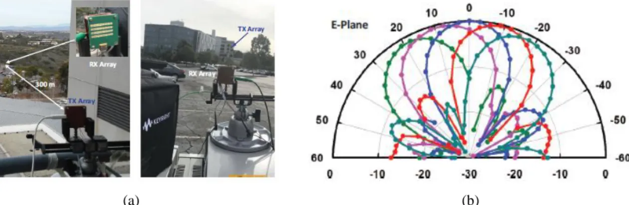
A 32-element phased-array transceiver for 5G communication links is presented in [14]. A 28 – 32 GHz silicon core chip is implemented with 4 transmit (TX)/receive (RX) elements, and 6-bit phase control. Eight of these chips are placed on a printed circuit board (PCB) with integrated antennas and Wilkinson combiners. The array is measured on both transmit and receive mode in a 300 m wireless communication as illustrated in Figure I-3(a). It demonstrated a measured EIRP (effective isotropic radiated power) of 41 dBm at P1dB and a beam scanning capability of ±20° and ±50° in E-, and H-planes, with a power consumption of 4.2 W and 6.4 W in RX and TX modes, respectively (Figure I-3(b)).

(37)

10

(a) (b)

Figure I-3: 28 GHz phased array transceiver. (a) Measurement setup. (b) E plane radiation pattern at 29.5 GHz.

Reflectarray antennas

Recently, some interesting architectures that demonstrate good performances for 5G applications have been presented in the open literature.

A single layer polarization independent reflectarray antenna working at 28 GHz for future 5G cellular applications is presented in [15] (Figure I-4). The array, which size is 10λ ×10λ, is composed of 400 unit cells. Each unit-cell contains three circular rings optimized to achieve linear phases by changing their size. The designed reflectarray is fed by a 12 dBi gain pyramidal horn having aperture dimensions of 14×12.4 mm2 with WR-28 waveguide. The CST software simulation results of the antenna exhibit a gain of about 25 dBi, and an efficiency of 58% at 28 GHz with E- and H-plane half-power beam-widths of 43.8° and 48.2°, respectively.

(a) (b)

Figure I-4: Single layer polarization independent reflectarray antenna. (a) Top view of the unit-cell. (b) Radiation patterns in E-plane.

A 38 GHz folded reflectarray antenna for 5G point-to-point communication is presented in [16]. It is composed of an upper reflector with a polarizing grid, a lower reflector with printed patches and a feed horn. The distance between the two reflectors is equal to 37.8 mm which corresponds to a focal length of 75.6 mm. The array has demonstrated a gain of 30.9 dBi, an