Comparison of receiver function deconvolution techniques

(1)

Comparison of Receiver Function Deconvolution Techniques

by

Kathryn A. Pesce

Submitted to the Department of Mechanical Engineering In Partial Fulfillment of the Requirements for the Degree of

Bachelors of Science in Mechanical Engineering at the

Massachusetts Institute of Technology September 2010

OCT

RARI

LI

BRARI ES

The author hereby grants to MIT permission to reproduce and to

distribute publicly paper and electronic copies of this thesis document in whole or in part in any medium now known or hereafter created.

Signature of Author...

Certified by...

Accepted by. ...

. ... . . ...

Department of Mechanical Engineering

August 23, 2010

....... ... . ... ...

Stephane Rondenay Department of Earth, Atmospheric, and Planetary Sciences Associate Professor of Geophysics Thesis Supervisor

... ... ...

John H. Lienhard V Collins Professor of Mechanical Engineering Chairman, Undergraduate Thesis Committee

(2)

(3)

Comparison of Receiver Function Deconvolution Techniques

by Kathryn A. Pesce

Submitted to the Department of Mechanical Engineering

On August 23, 2010 in partial fulfillment of the requirement for the degree of Bachelors of Science in Mechanical Engineering

Abstract

Receiver function (RF) techniques are commonly used by geophysicists to image discontinuities and estimate layer thicknesses within the crust and upper mantle. A receiver function is a time-series record of the P-to-S (Ps) teleseismic wave conversions within the earth and can be viewed as the Earth's impulse response. An RF is extracted from seismic data by deconvolving the observed trace from an estimate of the source wavelet. Due to the presence of noise in the data, the deconvolution is unstable and must be regularized. Six deconvolution techniques are evaluated and compared based on their performance with synthetic data sets. These methods approach the deconvolution problem from either the frequency or time domain; some approaches are based on iterative least-squares inversions, while others perform a direct inverse of the problem. The methods also vary in their underlying assumptions concerning the noise distribution of the data set, level of automation, and the degree of objectivity used in deriving or choosing the regularization parameter. The results from this study provide insight into the situations for which each deconvolution method is most reliable and appropriate.

Thesis Supervisor: Stephane Rondenay

Department of Earth, Atmospheric, and Planetary Sciences Associate Professor of Geophysics

(4)

Acknowledgements

I would like to thank my thesis advisor, Stephane Rondenay, for his invaluable guidance and support with this project and his wise academic and professional advice. Chin-Wu Chen provided much gracious assistance with the creation of the synthetic data. The infinite patience and kind backing of the Mechanical Engineering Undergraduate Office and my family greatly facilitated this project. I would also like to acknowledge the generous help of many friends who know the intricacies of MATLAB much better than I and whose quick tips and dirty tricks helped to get my code up and running.

(5)

List of Figures

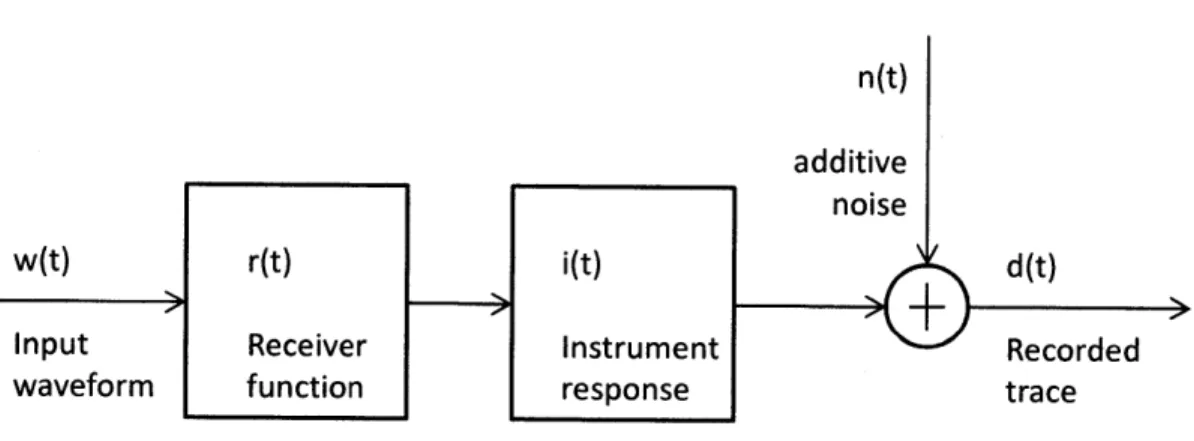
Figure 2-1: Block diagram modeling the system expressed by Eq. 1, in which the input source wavelet is sent through a set of linear systems, two convolution operators and a summation junction. The output is the recorded seismogram. In the actual case, the input and the recorded trace are known, and w(t) is deconvolved from d(t) to extract r(t), with special care taken to remove and adjust for the instrument response i(t) and noise input n(t)...10 Figure 2-2: Schematic diagram showing (a) the P to S conversion of an incident plane P wave on the

Mohorovic discontinuity adapted from Rondenay (2009), and (b) the seismic trace is the result of the

convolution of the RF with the source wavelet, which includes the instrument response and residual energy. The receiver function reflects the location and resolution of the underlying discontinuity. Figure adapted from Chung and Kanam ori (1980)... ₁₁ Figure 2-3: (a) Simple spectral division of synthetic and noiseless w and d results in the extraction of the

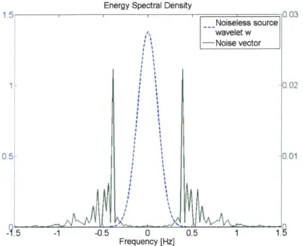
correct RF. (b) Spectral division of d and w with noise is unstable and fails...12 Figure 3-1: Comparison of energy spectral densities (ESD) of the noiseless source wavelet and the noise

vector. The ESD of the w Gaussian pulse in the time domain is a scaled Gaussian pulse in the frequency

domain. The noise vector introduces higher frequency components into the source wavelet so that the ultimate ESD of the noisy source wavelet is the summation of the two traces...14 Figure 3-2: Comparison of energy spectral density of deconvolution denominator before and after damping factor is added. Data4, 6 = 1000. The damping factor vertically shifts and broadens the spectrum to create a m ore effective low pass filter... 16 Figure 3-3: Evolution of the damping factor deconvolution of Data4. No significant change in RF occurred past 6=107_{. As 6 increases, the peaks lose resolution by broadening and shortening and the side lobes} diminish. Under 6=106, _{the energy spectral density of the denominator remained peaky, but it began to} flatten o ut above that value...17

Figure 3-4: Comparison of energy spectral density of deconvolution denominator before and after water

level operation. Data2, w ater level = 5e5... 18 Figure 3-5: Evolution of the water level deconvolution of Data4. No significant change in RF occurred past water level=107

. As the water level increases, the peaks lose resolution by broadening and

shortening and the side lobes diminish. The energy spectral density of the denominator flattened out to

a constant value above at a water level of 106 and above. ... 19

Figure 3-6: Illustration of GCV behavior and damping factor selection. A single trace results in a

flattening of the GCV curve, while stacked traces present a much clearer absolute minimum. The red "x" indicates the m inim um of the G CV...21

(7)

Figure 3-7: Illustration of GCV behavior and damping factor selection when the noiseless traces are input into the frequency domain damped least-squares deconvolution. The red "x" indicates the minimum of the G CV ...---...----.... ---... 22

Figure 3-8: Results of frequency domain array-conditioned deconvolution for Data4... 25 Figure 3-9: Evolution of the time domain simultaneous least-squares deconvolution of Data4 with and without noise. As p increases, the RF spikes are squeezed and resolution is increased. After ten iterations the RFs of the noisy data sets begin to lose their smooth shape. However, twenty iterations extracted the RF perfectly from the noiseless data sets... 27 Figure 3-10: Misfit trends of Data4 over 20 iterations. The misfit converges with increasing model size as the percent change between iterations drops below 0.5%...28 Figure 3-11: Time domain forward iterative deconvolution results for Data4 after three iterations. RF peaks are in correct locations, but amplitudes are slightly off. Results from all other data sets were approxim ately the sam e... ... --.... ....29 Figure 3-12: RF and misfit trends of Data4 over 7 iterations. Model size decreases over time and misfit does not converge... . -... --... ---... 30 Figure 4-1: Comparison of ESDs of the synthetic data sets: (a) source wavelets and source wavelet noise vectors and (b) observed traces and observed trace noise vectors. The energy of Data4, the multichannel, single-event set, is significantly more concentrated at lower frequencies than either Data2 or Data3. The noise vectors of Data4 and Data2 are almost equivalent, while the noise energy of Data3 is m uch higher...---.---... ---... 32 A ppendix 8 - Supporting figures...50

(8)

1. Introduction

Receiver function techniques are commonly used by geophysicists to image discontinuities and estimate layer thicknesses within the crust and upper mantle. A receiver function (RF) is a time-series record of the P-to-S (Ps) teleseismic wave conversions within the earth. As such, an RF can be thought of as the impulse response of the earth. According to seismic ray theory, the wave conversions are generated by discontinuities within the Earth's structure (Rondenay 2009). In general, a discontinuity is a rapid change in material properties due to variations in density, composition, and/or structure.

RFs are applicable for depths approaching the mantle transition zone, up to several hundred kilometers, and are widely used to determine lithospheric thicknesses and the depth of the Mohorovic discontinuity at various locations around the Earth. RFs are only appropriate for major discontinuities that can be approximated by a 1-D simplifying assumption (Rondenay 2009). Smaller discontinuities with lengths on the order of the wavelength of teleseismic waves require a fundamentally different approach known as migration techniques.

One of the earliest applications of RFs is described in a proof-of-concept paper authored by Vinnik (1977), in which he was able to accurately locate the 410 and 660 km discontinuities using Ps converted waves. RF techniques are somewhat depth-limited because phase conversions that may occur in the mantle are often overprinted by crustal reverberations that show up at the same time in the seismic trace; however, Bostock (1988) has developed improved methods of dealing with this overprint and applied RF analysis to characterizing the mantle stratigraphy of the Archean Slave province in the Canadian Shield.

More recent work has focused on the application of S-to-P (Sp) converted waves as a complementary RF technique. Sp wave conversions can be easier to identify in a seismogram because they arrive much earlier than their multiples and consequently escape distortion. While Ps waves are sensitive to sharp discontinuities, Sp phases have longer periods and, thus, are more adept at identifying gradational boundaries of material properties within the Earth structure (Vinnik 2007). Vinnik and Farra (2002) gained insight into the coupled motion of the lithosphere and underlying upper mantle by using RF techniques with Sp phases to study the relationship between approximately 200 Ma flood basalts in East and Southern Africa and the Tunguska basin of the Siberian platform and their underlying low S-velocity zones. Whereas RFs are attune to discontinuities in Earth structure, tomographic methods are sensitive to volumetric changes in material properties; thus, the two methods are used in tandem for solid earth imaging. Vinnik and Farra were able to further support their coupled motion theory with a tomographic model (VanDecar et al. 1995).

An RF can be extracted from seismic data by deconvolving the vertical component of a seismogram (an estimate of the source wavelet) from the horizontal component (the seismic trace). The RF peak arrival times correspond to the times of the wave conversions, thus, the depth of the discontinuity, and the RF amplitudes are proportional to the magnitude of the discontinuity (i.e., the gradient in seismic velocities and/or density). Due to noise present in the data deriving from the instrument response; surface

(9)

phenomena such as ambient noise, wind, or waves; and the fact that the source wavelet used in the deconvolution is only an estimate, the deconvolution problem must be regularized to avoid instability, and many methodologies have been developed to do so (Stein and Wysession 2003). These methods approach the deconvolution problem from either the frequency or time domain; some approaches are based on iterative least-squares inversions, while others perform a direct inverse of the problem. The methods also vary in their underlying assumptions concerning the noise distribution of the data set, level of automation, and the degree of objectivity used in deriving or choosing the regularization parameter.

The objective of this thesis is to evaluate and compare the advantages and weaknesses of six deconvolution methods. Within the frequency domain, the traditional damping factor and water level deconvolution methods are assessed, as well as the least-squares simultaneous deconvolution of Bostock (1998) and an array-conditioned deconvolution by Chen et al. (2010). We also evaluate two methods that treat the problem in time domain: another least-squares simultaneous deconvolution method of Gurrola et al. (1995) and a forward iterative method described by Liggoria and Ammon (1999). To conduct our study, we created a set of modular codes that encompass these deconvolution methods and tested each method using synthetic data sets. The synthetic data sets consist of both single traces and, where appropriate, multiple traces for stacked or simultaneous deconvolution. Although many papers have described individual deconvolution methods in detail, a rigorous comparison of the methods has not been completed. The results from this study provide insight into the

situations for which each deconvolution method is most reliable and appropriate.

2. Background

According to ray theory and the stress-strain boundary conditions that apply at welded boundaries, a wavefield interacts with a boundary by partitioning into both transmitted and reflected waves of various polarizations following conditions specified by the Zoeppritz equations (Aki and Richards 2002). For instance when a P-wave encounters an interface it transmits some energy through, including the Ps (also known as the vertical S-wave component or SV) and P phases and reflects others. The Ps conversion is advantageous because it arrives relatively early in the seismic record which prevents it being lost among the many later-arriving phases (Fowler 2005).

A broadband seismometer records data along three separate axes. Some pre-processing is necessary prior to deconvolution in order to separate the incident and converted wave phases. The simplest of these techniques involves recasting the seismometer traces into three orthogonal components aligned

in the radial, transverse, and vertical directions, and then relying on an assumption of a near-vertical incident P-wave (Rondenay 2009). The transmitted P phase is estimated to remain confined on the vertical component of the seismogram while the converted Ps contribution is on the radial component in isotropic media, which we will refer to as the horizontal component. The source wavelet, usually a distant earthquake, is not known and must be estimated from the available seismogram. The P-wave component is used as an approximation of the source wavelet because it is relatively unaffected by discontinuities, and the Ps phase is used as the recorded trace (Bostock 1998). More sophisticated techniques of isolating the source wavelet and trace minimize signal leakage between components of

(10)

the seismogram by rotating the components into the direction of polarization of the incident wave field (e.g., Langston 1979).

Linear system theory is a convenient and appropriate way of describing the behavior of seismic waves interacting with discontinuities because these Earth structures affect the waves according to the principle of superposition. A linear system is fully characterized by its impulse response. The output of a linear system corresponding to an arbitrary input signal is the convolution of that input with the system's impulse response. The Fourier transform also has linear properties; thus, Fourier analysis is a useful tool when coupled with linear system theory (Stein and Wysession 2003). The frequency-domain representation of the data are often complex numbers containing both the phase and amplitude information of the seismic waves. The phase and amplitude of the input waveform is transformed by the operators in the linear system to create the output.

The seismic trace, represented by the vector d (i elements), is the result of the convolution of the source wavelet w (n elements) with the RF or impulse response of the Earth r (m elements) (Berkhout 1977). The recording instrument, which in most cases is a 3-componenet broadband seismometer, has an

impulse response of its own that acts as another linear operator. Other sources of ambient noise and residual energy enter the seismic trace as noise and are added into the convolution as n (i elements).

d(t) = w(t) * r(t) * i(t) + n(t) (1)

n(t) additive

noise

WMt r(t) i(t) d (t)

Input Receiver Instrument Recorded

waveform L function Iresponse trace

Figure 2-1: Block diagram modeling the system expressed by Eq. 1, in which the input source wavelet is sent through a set of linear systems, two convolution operators and a summation junction. The output is the recorded seismogram. In the actual case, the input and the recorded trace are known, and w(t) is deconvolved from d(t) to extract r(t), with special care taken to remove and adjust for the instrument response i(t) and noise input n(t).

In general, convolution is defined as the integral of the product of two signals, one of which is flipped and shifted in the time domain (Bracewell 1986). According to the convolution theorem, convolution in the time domain is mapped as multiplication in the frequency domain. The seismic trace d can be thought of as a sliding average of the RF weighted by the source wavelet w . In the remainder of the text, we combine the convolved input waveform and the instrument response in w and refer to it as the

(11)

d(t) = w(t) * r(t) = f w(t - T)r(T)dr = F-(w(o) - r((2)

Deconvolution recovers the RF from the seismic trace by removing the effects of the input wavelet, the instrument response, and the residual noise. The RF is indicative of the Earth structure in the vicinity of the seismometer, so deconvolution is effectively source-normalizing the data (Fowler 2005). Because the effects of the input and the seismometer have been removed, the deconvolved data from various

sources and receivers can be compared directly.

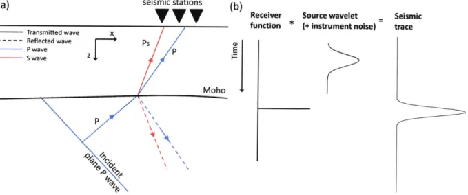
(a) seismic stations (b)

Receiver Source wavelet - Seismic

function (+ instrument noise) trace Transmitted wave X - - - - - Reflected wave Ps P wave Z S wave Z > Moho 0 P

Figure 2-2: Schematic diagram showing (a) the P to S conversion of an incident plane P wave on the Mohorovic discontinuity adapted from Rondenay (2009), and (b) the seismic trace is the result of the convolution of the RF with the source wavelet, which includes the instrument response and residual energy. The receiver function reflects the location and resolution of the underlying discontinuity. Figure adapted from Chung and Kanamori (1980).

Deconvolution is not a technique subject-specific to seismology. It is widely applied in optics and image processing to sharpen images and clear distortions. In order to regain the undistorted image, the output image is deconvolved by a point spread function (PSF) which mathematically describes the optical distortion pathway (Cheng 2006).

Deconvolution techniques are part of the larger category known as inverse problems that also includes tomography, remote sensing, and other geophysical methods. These are problems in which the mathematical model and observed data are known, and an estimate of the model parameters is extracted by fitting the data to the model (Lines and Treitel 1984). In RF analysis, the goal in solving an inverse problem is to characterize the medium through which the seismic wave phases traveled in terms of discontinuities and changes in material properties and velocity contrasts. The mathematical model used is the deconvolution operator, and the seismic traces serve as the observed data.

Inverse problems in Earth sciences are notoriously underdetermined. The data is always of finite length and often incomplete; thus, the result of an inversion is non-unique. Each solution to a given inversion has a distinctive balance resulting from the tradeoff between resolution and stability. Two general

(12)

strategies for solving inverse problems involve either directly solving for the model parameters by mathematical inverse techniques or iteratively solving the forward problem by estimating the model parameters, predicting the data, and evaluating the error between the observed and predicted data (Menke 1984). This study evaluates inverse deconvolution methods that follow both strategies.

Because deconvolution in the time-domain is equivalent to division in the frequency domain, straight spectral division of d by w, known as inverse filtering, would accurately produce the RF in the absence of

noise. However, noise of a relatively high frequency is always present in the trace. The source wavelet naturally acts as a low pass-filter; consequently, the inverse of w which is the operator in the deconvolution is effectively a high pass filter and amplifies the unwanted high-frequency noise (Gurrola et al. 1995). Small values of w in the denominator result in numerical instability in the RF, and it will approach infinity. Therefore, the deconvolution problem must be regularized. Many methodologies for doing so in both the frequency and time domains have been developed.

0.51 a> S0.5 (U E U_ 0 10 Time [s] Time [s]

Figure 2-3: (a) Simple spectral division of synthetic and noiseless w and d results in the extraction of the correct RF. (b) Spectral division of d and w with noise is unstable and fails.

Another factor limiting the accuracy of the deconvolution is that the w used is merely an estimate of the actual source signature, as discussed previously. The deconvolution is not totally blind, but the exact w

is not known and, thus, has inherent inaccuracies that propagate into the RF (Rondenay 2009).

(13)

Two of the earliest-developed deconvolution techniques, referred to in this paper as water level deconvolution and damping factor deconvolution, draw directly from the work of the mathematician Norbert Wiener. Wiener deconvolution is a non-iterative, direct inverse technique that operates in the frequency domain to reduce the effect of noise in the deconvolution (Wiener 1964). The filter applied is based on the mean power spectral density of the noise, which is assumed to be white Gaussian noise and independent of the input. The strength of the filter is inversely related to the signal-to-noise ratio (SNR) of the data, so when the SNR is very high (when there is little noise present in the data), the effect of the filter is weakened so the deconvolution is almost identical to a direct spectral division.

The first applications of Wiener deconvolution to RF analysis were not data-adaptive, meaning that the filter was not designed to self-adjust and be optimized for variable inputs (Langston 1979). Later work on deconvolution techniques developed methods that are data-adaptive and some that are customizable to address specific shortcomings in the data. Bostock (1998) crafted a frequency domain technique evolved from Wiener deconvolution that allows for the optimization of the damping factor by a least-squares inversion to minimize the generalized cross-validation function (GCV). Recently, Chen et al. (2010) has created and applied a data-adaptive, spectral division filter. Within the time domain, the method of Gurrola et al. (1995) attempts to solve the deconvolution by a least-squares inversion aimed at minimizing the difference between the recorded data and an estimated data set based on the calculated RF. The time-domain deconvolution method of Liggoria and Ammon (1999) is constructive. By iteratively extracting the most highly cross-correlated signal and using that information to fit spikes to

reconstruct the Earth's impulse response, the method solves the forward problem by building the RF until a specified misfit is reached.

Research continues on the improvement of RF methods. The evolution of RF techniques has been aimed towards augmenting their data adaptability and increasing the degree of objectivity in the choice of regularization parameter. In the early RF techniques, such as water level and damping factor deconvolution, we directly exert control over the problem by manually selecting the regularization parameter. More sophisticated methods take advantage of the properties of the data set to optimize the regularization parameter automatically.

The robustness of these methods is enhanced both in the frequency and time domains by pre-deconvolution stacking and simultaneous pre-deconvolution. RF techniques were created to detect weak secondary signals in which the signal to noise ratio is often low, so simultaneously deconvolving multiple traces related to the same RF increases the strength of the signals and thus the strength of the result as well (Gurrola et al. 1995; Bostock 1998). Some techniques are tailored towards evaluating multiple events recorded at a single station, whereas others look at a single event recorded at multiple stations.

3. Methods

In the following sections, each of the deconvolution methods are discussed in detail and the deconvolution results are given. First, however, we describe the methodology used to create the synthetic data sets.

(14)

3.1 Synthetic data

It is common to use synthetic data sets to assess the viability of deconvolution methods. Usually, the data is constructed to emulate hypothetical but realistic earth structure and seismic velocities (e.g., Liggoria and Ammon 1999; Chen et al. 2010) However, in this paper we decided to use very simple synthetic data sets in order to set an initial benchmark for each of the methods (see Figure 2-3(a)). The data were built by forward modeling of the observed trace through the convolution of the source wavelet, a simple Gaussian pulse, with the RF, a series of concatenated peaks. The independent noise vectors added to d and w, as seen in Figure 2-3(b), are pre-event noise extracted from actual seismograms. The pre-event noise was extracted from the real seismogram, normalized to one, and then randomly shifted in time. Thus, the term "noise level" refers to a percentage of the normalized noise vector's amplitude. The goal of the deconvolution is to recover the RF as seen in Figure 2-3(a) as accurately as possible. The synthetic RF has a peak with a magnitude of one at five seconds, followed by a peak of magnitude -0.4 at eighteen seconds.

Energy Spectral Density

1.5 0.03 Noiseless source wavelet w -Noise vector 10.02 0.5 0.01 5 1 -0.5 0 0.5 1 1. Frequency [Hz]

Figure 3-1: Comparison of energy spectral densities (ESD) of the noiseless source wavelet and the noise vector. The ESD of the w Gaussian pulse in the time domain is a scaled Gaussian pulse in the frequency domain. The noise vector introduces higher frequency components into the source wavelet so that the ultimate ESD of the noisy source wavelet is the summation of the two traces.

For simultaneous deconvolution, which all six methods in this paper accommodate, multiple traces are grouped as a matrix data set and delivered to the inverse operator for processing. To examine the scenario in which the same event was recorded at many stations (single event, multichannel), the same Gaussian pulse w and convolved trace d were used in all twenty traces but distinct noise was added to each trace. Different sets with varying amounts of noise were created. Another data set was created to imitate many different earthquake events recorded at the same station (single channel, multi-event). This is the more common way of evaluating simultaneous RFs (Bostock 1998). A group of Gaussian

(15)

pulses with diverse characteristics were individually convolved with the same RF to produce the set of observed traces. Again, separate noise was added to each trace.

There are four data sets used to test the code referred to throughout the remainder of the paper which are described as follows. Each member of a data set consists of the observed trace d and its corresponding source wavelet w. They were all constructed using the same RF (seen in Figure 2-3(a)) and independent noise vectors were added to each w and d. Datal is a single trace. Data2 imitates a single event, multichannel data set. It is a set of twenty pairs with a 20% noise level. Data3 was constructed by the same process as Data2 but with a noise level of 30%. Data4 is also twenty pairs of traces and mimics a single channel, multi-event data set with a 20% noise level.

3.2 Damping factor deconvolution

The damping factor deconvolution method is derived directly from Wiener deconvolution. As in Wiener deconvolution, the noise spectrum is assumed to be Gaussian random noise with zero-mean (Wiener 1964). The RF is produced by a modified spectral division as shown in Eq. 3, where the asterisk denotes the complex conjugate and the regularization parameter is cast as the damping factor 6 (Gurrola et al.

1995).

f~o) r = (w) d(oi)w*(w) a)

(

₍₃₎

w(w)w*(w) + 6

The damping factor effectively prewhitens the power spectrum in the denominator and prevents the instability that would be caused by small values. The inclusion of 6 is equivalent to adding white noise to the signal and effectively shifts the power spectrum of the denominator (the auto-correlation of the input) vertically (Lines and Treitel 1984). It also broadens and boosts the height of the spectrum to increase the bandwidth. The filter is the inverse of the denominator, so in actuality the addition of 6 is enhancing its effectiveness as a low pass filter. As 6 approaches zero, Eq. 3 is akin to pure spectral division. As 6 becomes large and nears the maximum value of the original spectrum, the power spectra flattens out and the denominator is approximately a constant value. Damping factor deconvolution can also be viewed as the cross-correlation of the output d with the input w normalized by the damped autocorrelation of the inputs (Gurrola et al. 1995).

(16)

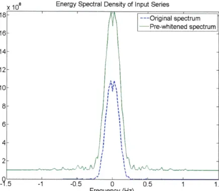
Energy Spectral Density of Input Series

-1.5 -1 -0.5 0 0.5 1 1.5

Frequency (Hz)

Figure 3-2: Comparison of energy spectral density of deconvolution denominator before and after

damping factor is added. Data4, 8 = 1000. The damping factor vertically shifts and broadens the

spectrum to create a more effective low pass filter.

The damping factor can be selected as a percentage of the mean power spectral density of the noise, but we often choose it semi-arbitrarily on a trial and error basis to balance the noise level, the peak, and the side lobe resolution. The damping factor changes the nature of the input from a high pass filter to a low pass filter; therefore, it reduces the impact from the high-frequency noise and cuts the frequency content of the resultant RF. Since the RF is essentially a delta function, it has content at all frequencies, so a tradeoff of the technique is that some of the high frequency content of the RF is also lost, reducing the amplitudes of the deconvolved signals.

Single-events can be processed individually according to Eq. 3 and then stacked afterwards; however, stacking prior to the spectral division improves the SNR and reduces the strength of damping needed (Bostock 1998). Eq. 4 describes the simultaneous deconvolution. M is the total number of traces, and m is the number of the individual trace.

Zn=1dm(w)w* (&)

r(W) = (Z= (4)

& =1WM (CO)w 4M) +

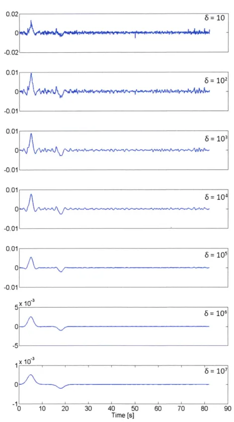
From the RF evolution of Data4 shown in Figure 3-3, it can be seen that a 6 of approximately 104 _is

desirable for stabilizing the spectral division. This value reduces the presence of the residue side lobes, but does not broaden the RF peaks unreasonably.

(17)

6= 10 0.0 -0.0' 0.01 6= 101 0 -0.01 0.01 0 = 104 -0.01 -11 0 10 20 30 40 50 Time [s] 60 70 80 90

Figure 3-3: Evolution of the damping factor deconvolution of Data4. No significant change in RF occurred

past 6=107. As 6 increases, the peaks lose resolution by broadening and shortening and the side lobes

diminish. Under 6=106, the energy spectral density of the denominator remained peaky, but it began to flatten out above that value.

-0~10w VOW

0.02

(18)

Data2 requires a similar damping factor for stabilization; however, the RF results of Data4 retain more of the peaked nature and amplitude of the original RF than either Data2 or Data3. Data3, characterized by

the higher noise level, requires a 6 of approximately 105 to achieve similar results. Datal necessitates a

damping factor of comparable magnitude to Data4; however, its results lose even more amplitude information, as expected since it is only a single trace. Also, although Datal has less of an issue with side lobes, the resolution of peak locations is poorer at low damping factors. The RF evolutions for all data sets are in Appendix B-1.

3.3 Water level deconvolution

Water level deconvolution is very similar in practice to damping factor deconvolution. Instead of adding a regularization parameter to every entry in the denominator, values below a specified threshold are replaced with a chosen water level value (Menke 1984). Again, water level deconvolution acts as a low pass filtering technique; however, it has a visually different effect on the energy spectral density of the spectral division denominator. Unlike the addition of a damping factor, the application of a water level does not broaden or heighten the peak of the energy spectral density. Above the water level, the ESD is identical to its original form. The water level increases the bandwidth of ESD by including an equal amount of all frequencies present below the water level.

x 1ol Energy Spectral Density of Input Series

I I

0.5F--0.5 0

Frequency (Hz) Figure 3-4: Comparison of energy spectral density of deconvolution level operation. Data2, water level = 5e5.

denominator before and after water

If the water level is large, the power spectrum of the denominator will approach a constant value. Choosing a water level is again a subjective task in which the noise level, peak resolution, and side lobe

---Original spectrum

-Pre-whitened spectrum

--

rgnlsetu

(19)

-occurrence are visually balanced by the user. A water level of approximately 104 _{suitably stabilizes the}

deconvolution of Data4.

Water Level Deconvolution

10 20 30 40 50 60 70 80 90

Time [s]

Figure 3-5: Evolution of the water level deconvolution of Data4. No significant change in RF occurred

past water level=107. As the water level increases, the peaks lose resolution by broadening and

shortening and the side lobes diminish. The energy spectral density of the denominator flattened out to

a constant value above at a water level of 106 and above.

The results of the data sets relative to each other mimic those of the damping factor deconvolution results. The RF evolutions for all data sets are in Appendix B-2.

(20)

3.4 Frequency domain damped least-squares deconvolution

The method employed by Bostock et al. (1998) is identical to the simultaneous damping factor deconvolution described above, except that the damping factor is not chosen by the user. Instead, the 6 considered optimal is the one which minimizes the General Cross Validation function (GCV). The GCV is defined as V)1 i=1(dm(wn) - wm(wn)r(On))( GCV(8) = = E ₍₅₎ (MN -E= 1 X(O)) 2 X(O) = (6) (ZE=1 iwm(W)W,* (()) + 8

where Nis the number of frequencies represented by the Fourier transform, Mis the number of traces,

and o is the frequency. .

The GCV is a form of regularization drawn from regression analysis. The iterative grid search is begun by choosing a starting value of 6 and then forward modeling to obtain a prediction of the data. The numerator of the GCV in Eq. 5 is the residual sum of squares (RSS). The RSS assesses the discrepancy between the predicted and observed data and is essentially an estimate of the goodness of fit of the model. The calculation in the denominator involving the degrees of freedom of the model is used to balance the fit and the model size or complexity (Hastie et al. 2009). The iteration continues over a range of 6 values. Finally, the optimal regularization parameter corresponding to the minimum GCV is used in Eq. 4 to complete the deconvolution. Special care should be taken to ensure that the step size of the iteration allows adequate resolution and that the minimum 6 does not lay either bound of the search.

A white noise spectrum, implying a flat power spectral density, is assumed to be present in the data set; however, this does not include specific assumptions about the noise level or amplitude distribution (Bostock 1998).

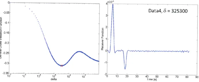
The results from testing this deconvolution technique with the synthetic data sets are interesting. The method selected regularization parameters for Datal and Data3 that are smaller by an order of magnitude than those selected for Data2 and Data4, even though the properties of the latter two data sets, namely the noise level and amount of traces, are considered more desirable for deconvolution. The appearance of the generated RFs is acceptable. The peaks are in the correct locations and clearly discernible, and the side lobes have been greatly reduced. However, the Data3 RF is considerably noisier than the others. Stacking traces substantially affects the form of the GCV. For an individual trace, the GCV has an extremely subtle, almost flat absolute minimum, but the stacked traces prompt the GCV to display a much sharper minimum.

(21)

0 . 1 - 15 C 0) G, -2 -102 x10-4 Datal, 5 = 558 10 40 60 70 Time IS] 00 30

M~r

so 90 Data2, S = 201000 x103 Time [s] delta 10 10 10 delta ... n CL

(22)

0 -0.13 -03 25 -(DL S-0.2[ 10' 0 1 10 10 10 defta

Figure 3-6: Illustration of GCV behavior and damping factor flattening of the GCV curve, while stacked traces present a much indicates the minimum of the GCV.

selection. A single trace results in a clearer absolute minimum. The red "x"

Inputting noiseless synthetics into the method does not result in an optimal damping factor of zero, even though this would produce the RF exactly. Alternatively, the clean data set prompts the GCV to oscillate with very small amplitudes and eventually settle around zero. Thus, the damping factor selected corresponds to the value of the maximum negative oscillation and is sometimes greater in value than the damping factor selected for identical data sets that include the noise vectors.

2xl 10 x1_0-3

1.5 5 Data2 without noise, 6= 30000

C 4- 0.5-0 >L3 Uj-0.5 0 -ii d) 10 d delta 10 20 30 40 50 60 70 80 Time [s] .. ... ...

(23)

0 3 1.5-C .0 -1 0- - 5 -00.5 -M 0.5-00 -0.5- -2.5-2 0 10 20 30 40 50 60 70 80 90 delta

Figure 3-7: Illustration of GCV behavior and damping factor selection when the noiseless traces are input into the frequency domain damped least-squares deconvolution. The red "x" indicates the minimum of the GCV.

Because this deconvolution technique employs an iterative grid search, the run-time can be significant depending on the size of the data set, the bounds, and the step size selected for the search. The method also hinted at slight instability. When a data set identical to Data2 but with different noise vectors served as the input to the function, the minimum GCV was on the lower bound of the search at a 6 of approximately 100 which in reality was insufficient for stabilization. There was a local minimum present

in the GCV curve at a more appropriate damping factor of approximately 105. The results of all data sets

including their respective energy spectral density curves are in Appendix B-3.

3.5 Frequency domain array-conditioned deconvolution

In the three frequency domain methods previously described, the inverse filtering was accomplished by the addition of a regularization parameter of constant value in order to create a bandwidth-limited or

notch filter. On the other hand, the array-conditioned deconvolution create.s an optimal inverse filter that is automatic in nature, data-adaptive, and independently determined for each frequency present in the Fourier transform (Chen et al. 2010). The filter makes no assumptions about the distribution of the

noise and instead determines the relevant noise properties and uses them to regularize the problem. Array-conditioned deconvolution is unique in that it is biased toward multichannel processing, whereas most simultaneous deconvolution techniques are reported as preferring single channel, multi-event data (Chen et al. 2010).

The filter is derived from and determined directly by the model presented in Eq. 1. The goal of the filter is to minimize the noise energy and the energy attributed to the instability of the filter and to maximize the signal energy (Haldorsen et al. 1994; Haldorsen et al. 1995). It also seeks to compress and amplify the signal energy to create the spikes of the RF. These two conflicting concerns result in the deconvolution filter W(co).

. ... .. ... ... .. .... ... .

(24)

-w*(co)

W ':) =W _|_Iwo)12W(j _{+ EN(W)} (7)

EN(w) _{is the average total energy of the noise. Eq. 7 has a form identical to that of the inverse filter}

used in damping factor deconvolution if EN(w) were a constant value 6. EN(w) is not explicit, so the filter is reworked to include the average total energy of the raw traces ET(w) instead. The filter can

then be applied to the sum of stacked observed traces in order to estimate the RF.

W() = 0)(8) The average total energy of the raw traces is easily calculated as

ET() = Mm2 ₍₉₎

The filter can be rearranged again to give a more intuitive understanding of its function. It is the traditional inverse filter used in other forms of frequency domain deconvolution weighted at each

individual frequency by the semblance D(w).

Wfiter(OJ) = D(w) (10)

The semblance is a measure of signal coherence and is also related to the signal-to-noise ratio. It compares the energies of the input and the output and is, thus, telling of how much of the output can be predicted by the input at any given frequency (Haldorsen 1994).

Iw()12 ET(W)((11)

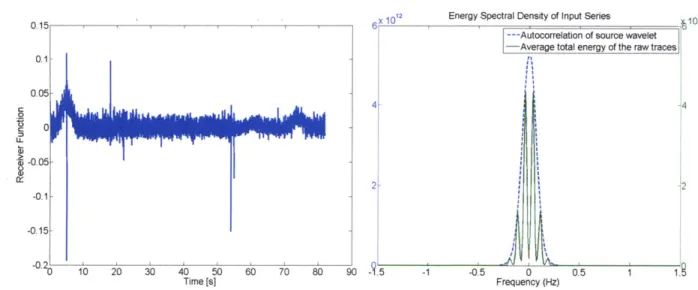
Overall, the array-conditioned deconvolution did not adequately extract the RFs from the synthetic data sets. Deconvolution of a single trace, Datal, produced no usable results, and the deconvolution also failed for noiseless data sets. The deconvolution of the stacked data sets accurately placed the first peak of the RF, but with poor resolution. The second RF peak was not recovered in any of the results. A strange artifact related to the folding of the Fourier transform is present in the last thirty seconds of each RF.

(25)

12 Energy Spectral Density of Input Serie010

--- Autocorrelation of source wavelet -Average total energy of the raw traces

0.1 -0.05 C 44 .0 0 -0.05 2- 2 -0.1 -0.15 .0 10 20 30 40 50 60 70 80 90 -. 5 1 -0.5 0 0.5 1 1.9 Time [s] Frequency (Hz)

Figure 3-8: Results of frequency domain array-conditioned deconvolution for Data4.

In other frequency domain deconvolution techniques, the denominator of the spectral division consisted

of the damped autocorrelation of the source wavelet. In array-conditioned deconvolution, ET(w) takes

up this role. The ESD of ET(co) has a drastically different appearance than that of the damped

autocorrelation seen previously. Instead of surpassing the undamped autocorrelation (the original spectrum) in magnitude, its magnitude is actually lower, and the peak did not broaden to include any additional higher frequency content. All data sets are available in Appendix B-4.

3.6 Time domain simultaneous least-squares deconvolution

The damped least-squares deconvolution in the time-domain serves the same purpose as the equivalent technique in the frequency domain, but it takes on a slightly different form of regularization. Due to its iterative nature, it does have an extended run-time; however, it also has increased flexibility and adaptability.

Each individual source wavelet w is recast into its own matrix W (Gurrola et al. 1995). The matrix has as many columns as the length of the resultant RF and as many rows as the length of the observed trace d. Each column contains the estimation of the source wavelet and trailing zeros.

W= ii 0 . 0 W 0 (12)

0

0 w 0 0 I * * 0 _it 1 .: - ...- --.- . -.- .. ..... I ... .... .... .- ::..::::::::::::: = .. ... .... .... . .. ... .... _ __ .mu -w:::wl -:: ---:::::: ::::::::::::::::::::::::::::::::::::::: , :::::::::::.:::::- ,

(26)

The inversion attempts to minimize the error or RMS difference between the prediction of the data and the observed data (also known as the misfit). Just as in the frequency domain techniques, this solution is not unique and has potential for instability due to the presence of noise. Therefore, the problem must be regularized by some inherent aspect of the data or the inversion. For example, we regularized the problem by the size of the RF, which is directly proportional to its energy. The regularized cost function (Eq. 13) balances the misfit with the RF size, imposing a condition of minimum energy (Rondenay 2009). A Lagrange multiplier u is used to weight both the misfit and the model size constraint. The Lagrange

multiplier is analogous to the water level or damping factor utilized in frequency domain techniques.

||Wr - d| 2 ₊_p2||r||2 ₍₁₃₎

This deconvolution technique is adaptable and versatile because different aspects of the inversion, essentially various model norms, can be chosen as the regularization parameter in order to address specific problems of smoothness or size within the data set (Gurrola et al. 1995). Following Eq. 13, the cost function is then differentiated and set equal to zero in order to derive the weighted least-squares solution (Gurrola et al. 1995).

r = (WTW + pt2 1)-1WTd (14)

p _{is decreased by an order of magnitude every iteration until misfit convergence is reached. The criteria} for convergence is defined by the percent change of the misfit from one iteration to the next. When it drops below an acceptable value, usually 0.05%, the algorithm is halted. A conventional initial value of the Lagrange multiplier is 100, and the misfit typically converges after about eight to twelve inversions (Gurrola et al. 1995). The method is easily extended to a simultaneous deconvolution preferring single channel, multi-event data sets.

r= (M=1 WmTWm + p21) um Wm dm (15)

A Lagrange multiplier of about 10 to 1000, corresponding to eight to ten iterations, regardless of noise level or multi/single channel data sets, was sufficient to recover the RFs for all of the synthetic data sets. The general, smooth shape of the RF was extracted after only the second iteration. However, increasing p results in enhanced resolution as the RF peaks narrow and heighten, with optimal resolution achieved at eight to ten iterations. After ten iterations, the recovered RF peaks continue to taper and squeeze, but overall the RFs actually appeared to get noisier and lose their smooth shape. In the test in which a noiseless data set served as the input, twenty iterations recovered the RF exactly. However, twenty

(27)

107 Data4 1Data4 . without noise 4p 1L09 2= 4= 109iter 2iterations 4 2 iterations 2- 2 14 -4 X lp=X10 5iterations 18 iterations 0 0 . 1 --- 2 10ieatos 0.0120iertos 010 1 00 20 iterations 05- 20 iterations -05 o 10o 2 o5 5 10 15 20 25 Time [s] Time [s]

Figure 3-9: Evolution of the time domain simultaneous least-squares deconvolution of Data4 with and without noise. As u increases, the RF spikes are compressed and resolution is increased. After ten iterations the RFs of the noisy data sets begin to lose their smooth shape. However, twenty iterations extracted the RF perfectly from the noiseless data sets.

The misfit-RF size trend (see Figure 3-10) is consistent with what is found in the literature, and the misfit does converge as the size of the model grows (Gurrola et al. 1995). A percent change of 0.05% proved too extreme to ever result in convergence, so 0.5% was used instead. For all Data sets, this benchmark corresponded to eight or nine iterations. All data sets are available in Appendix B-5.

(28)

Data4

p= 10) 2.5

3 20 iterations

02

D2d05 0.1 0,015 0,02 0.025 OM 0.035 004 0.45 4 8 1 12 14 1 18 20

Model Size 11rfl2 Iteration

Figure 3-10: Misfit trends of Data4 over 20 iterations. The misfit converges with increasing model size as

the percent change between iterations drops below 0.5%.

3.7 Time domain forward iterative deconvolution

The time-domain forward iterative approach is the only deconvolution technique presented in this paper that does not provide a form of regularization. The method developed by Kikuchi and Kanamori

(1982) and Ligorria and Ammon (1999) attacks the deconvolution by iteratively constructing the RF

instead of mining the data in order to extract it.

The technique relies on the cross-correlation function, which measures the similarity of two waveforms as a function of a time-lag applied to one of them. It is the integral of the product of two signals, one of which is shifted in the time domain. It is related to convolution except the shifted signal is not also flipped (Bracewell 1986). Cross correlation in the time domain is equivalent to multiplication with a

conjugate complex in the frequency domain.

(w * d) (t) = Ef_ w*(T ) d(t + T ) dT ='-w() (16 dT)

To proceed with this technique, the vertical and horizontal components of the seismogram are cross-correlated. An RF peak is placed at a time lag corresponding to the point of maximum cross correlation. Then this estimate of the RF is convolved with the source wavelet to create a prediction of the observed trace, and the result is subtracted from the original observed trace. This process is iterated until a certain value of misfit is reached (Liggoria and Ammon 1999). Once the new RF spikes being added are insignificant in size, the method terminates. The amplitude of each RF spike is related to the maximum cross-correlation coefficient and can be estimated according to the method described by Kikuchi and Kanamori (1982).

The method prioritizes by focusing first on the most important and energetic features and then shapes the smaller details and is inherently more stable because of this. The RF lacks the side lobes present in the results from other techniques because the shape of the RF peaks is pre-defined by the operator.

(29)

Regardless of which data set was input, the method consistently produced the same RF, differing only slightly in peak amplitude. Only three iterations, corresponding to a change in the misfit of 0.5%, were needed in most cases. After three iterations, the peaks added were most likely related to cross-correlation of the noise and were of significantly smaller amplitude than the true RF peaks. An example of the evolution of the cross-correlation, RF estimate, and convolved trace over three iterations for Data4 is in Appendix B-6. C 0 Data4 o 6e 3 Iterations 0.2-o _0.2 4 5 10 15 - Tine [s

Figure 3-11: Time domain forward iterative deconvolu peaks are in correct locations, but amplitudes are slig approximately the same.

20 2 30 35

tion results for Data4 after three iterations. RF htly off. Results from all other data sets were

There was a slight failure of the misfit convergence criteria when using this technique. The RF size seems to strangely decrease as the iterations progress, and the misfit does not appear to approach convergence. The misfit may tend towards a constant value eventually; however, it was difficult and very time-consuming to run the method for more than seven iterations because within each pass the data set was padded with zeros to maintain proper matrix dimensions. After seven iterations the length of the data set was unwieldy and the computation time was extremely lengthy.

(30)

Ddta4 08 7 iterations 06. 2.! 504,2 02-3 1 1 10 2 2 n2 32 3 2 0 C! 1 2 25 4 5 8 7 111118 Iod,1 Sao gr 1 11818101

Figure 3-12: RF and misfit trends of Data4 over 7 iterations. Model size decreases over time and misfit does not converge.

4. Discussion and conclusions

What remains to be discussed after a review of each individual technique is a comparison of the methods. A single objective metric on which to focus the discussion is difficult to pinpoint, and it is not clear that such an ideal metric exists yet, especially one that evaluates both the time and frequency domain equitably. Many scientists tend to favor a certain method for arbitrary reasons and have not explored the full realm of RF deconvolution techniques, but it should be remembered that each has its appropriate time and place. For the synthetic data sets used in this paper, most techniques gave competitive results.

An exception to the above was the array-conditioned deconvolution. It is unique in that it is geared toward multi-channel use. In this paper, the synthetic data sets used are not well-suited for this technique so its execution was poor. In Chen et al. (2010), the authors do show successful implementations of the method with both synthetic and real data sets.

A few of the many standards or priorities that drive the choice of deconvolution technique include degree of objectivity, level of automation, resolution of RF, and speed. If speed and procuring a quick result are valued, then damping factor, water level, or array-conditioned deconvolution are appropriate because they are not iterative and, thus, are essentially immediate. However, many geophysicists steer clear of water level and damping factor because the techniques are considered too labor-intensive or subjective due to their guess-and-check nature. The trend is overall towards more automated methods that may require more time but also have the ability to regularize the deconvolution implicitly and produce repeatable results.

The frequency domain techniques suffer more from side lobe residue at the base of RF peaks because of numerical artifacts from the FFT. The damping factor produced slightly better results than the water level technique for all synthetic data sets, but the differences were not very significant. It is reasonable to view the iterative damped least-squares technique proposed by Bostock et al. (1998) as objective check on the damping factor and water level technique since it self-selects the damping factor based on the minimization of the GCV. However, in this study the methods gave almost opposing results. We

(31)

manually chose higher damping factors for Datal and Data3, while minimizing the GCV dictated a higher damping factor for Data2 and Data4. Thus, the method of Bostock et al. (1998) did not provide confirmation for our choice of damping factor, but it did produce acceptable RFs. The iterative damped least-squares method can be time-intensive and there is always the danger that the search is too limited and the minimum selected is only local or on the border of the search.

The time domain methods require a longer run-time but offer more flexibility and reduce the existence of side lobes. They are also desirable because they are fully-automated and provide an objective mechanism for stopping the iterations - the percent change of the misfit. The time domain iterative least-squares method of Gurrola et al. (1995) is very malleable. Although only model size (or the condition of minimum energy) was explored in this paper, the method can be regularized with a variety of norms depending on the characteristics of the data.

Because the user can self-select the shape of the RF peaks, the results of the time domain method presented by Liggoria and Ammon (1999) verge on looking almost too good and give a sense of false security. However, the forward method is preferable when the data set is small or smaller events are being used because it spikes the major features of the RF first before looking at the smaller details (Liggoria and Ammon 1999).

There are some very clear conclusions regarding the use of the synthetic data sets. Stacking reduced the presence of side lobes and generally increased the resolution of the RF and the efficiency of each technique to recover it. Moreover, the multi-event, single channel data set (Data4) outperformed the other stacked sets. Some insight can be gained by considering the energy spectral densities of the synthetic data sets. The ESD of Data4 is more highly concentrated at lower frequencies, so any low pass filtering technique would be more effective with this data set.

(32)

0 7 Energy Spectral Density of Source Wavelets

) T I- Data2

(a)-Dt

-0.4 -0.2 0 02 0.4 0.6 -15 -1 -0.5 0 0.5 1 1.5

x 107 Energy Spectral Density of Observed Traces Frequency [Hz}

(b) -Data3 -Data2 5 - Data4] 3 Data4

2.5-4-I

2-3

1

0.5.~.

f

0 A5 -04 -0.2 0 0.2 0.4 0.6 -5 -1 -0.5 0 0.5 1 15 Frequency [Hz] Frequency [Hz]

Figure 4-1: Comparison of ESDs of the synthetic data sets: (a) source wavelets and source wavelet noise

vectors and (b) observed traces and observed trace noise vectors. The energy of Data4, the multichannel, single-event set, is significantly more concentrated at lower frequencies than either Data2 or Data3. The noise vectors of Data4 and Data2 are almost equivalent, while the noise energy of Data3 is much higher.

The time domain methods were more adept at recovering the absolute magnitude of the RF peaks. Regardless, all techniques reliably produced the relative peak magnitudes.

More rigorous testing of the deconvolution techniques is warranted. Both synthetic and real data sets tailored to specific circumstances would aid the exploration of each deconvolution technique's niche. For example, similar testing could be completed on the frequency domain technique of Park and Levin

(2000) which performs the inversion with multi-taper correlation estimates damped according to the

pre-event noise spectrum. Also, more examination into multi-channel deconvolution methods could broaden the application and usability of RF techniques. Along with more advanced testing will come the development of an increasingly objective metric with which to compare the results.

(33)

References

Aki K, Richards PG (2002) Quantitative seismology, 2nd ed. University Science Books, Sausalito, CA Berkhout AJ (1977) Least-squares inverse filtering and wavelet deconvolution. Geophys 42:1369-1383 Bostock MG (1998) Mantle stratigraphy and evolution of the Slave province. J Geophys Res 103(B9): 21183-21200

Bracewell RN(1986) The Fourier transform and its applications, 2nd ed. McGraw-Hill Book Company, New York, NY

Chen CW, Miller DE, Djikpesse HA, Haldorsen JBU, Rondenay S (2010) Array-conditioned deconvolution of multiple-component teleseismic recordings. Geophys J Int 182:967-976

Cheng PC (2006) "The Contrast Formation in Optical Microscopy", Handbook of Biological Confocal Microscopy (Pawley JB, ed.), 3rd ed. Berlin: Springer, 189-90

Chung W-Y, Kanamori H (1980) Variation of seismic source parameters and stress drops within a descending slab and its implications in plate mechanics. Phys. Earth Planet. Inter. 23:134-59

Fowler, CMR (2005) The solid earth: and introduction to global geophysics, 2nd ed. Cambridge University Press, New York, NY

Gurrola H, Baker GE, Minster JB (1995) Simultaneous time-domain deconvolution with application to the computation of receiver functions. Geophys J Int 120:537-543

Haldoresen JBU, Miller DE, Walsh JJ (1994) Multichannel Wiener deconvolution of vertical seismic profiles. Geophys 59:1500-1511

Haldoresen JBU, Miller DE, Walsh JJ (1995) Walk-away VSP Using drill noise as a source. Geophys 60:978-997

Hastie T, Tibshirani R, and Friedman JH (2009) The elements of statistical learning: data mining, inference, and prediction, 2nd ed. Springer, Stanford, CA

Kikuchi M, Kanamori H (1982) Inversion of complex body waves. Bull Seismol Soc AM 72(2):491-506 Ligorria JP, Ammon CJ (1999) Iterative deconvolution and receiver-function estimation. Bull Seismol Soc Am 89(5):1395-1400

Langston CA (1979) Structure under Mount Rainier, Washington, inferred from teleseismic body waves. J Geophys Res 84(B9):4749-4762

Lines LR, Treitel S (1984) Tutorial a review of least-squares inversion and its application to geophysical problems. Geophys Prosp 32: 159-186

(34)

Menke, W (1984) Geophysical data analysis: discrete inverse theory. Academic Press, Inc., New York City, NY

Park J, Levin V (2000) Receiver functions from multiple-taper spectral correlation estimates. Bull Seismol Soc AM 90(6):1507:1520

Rondenay S (2009) Upper mantle imaging with array recordings of converted and scattered teleseismic waves. Surv Geophys 30:377-405

Stein S, Wysession, M (2003) An introduction to seismology, earthquakes, and earth structure. Blackwell Publishing, Malden, MA

Wiener N (1964) Extrapolation, interpolation, and smoothing of stationary time series: with engineering applications. MIT Press, Cambridge, MA

VanDecar JC, James DE Assumpcao M (1995) Seismic evidence for a fossil mantle plume beneath South America and implications for plate driving forces. Nature 378:25-31

Vinnik L (1977) Detection of waves converted from P to SV in the mantle. Phys Earth Planet Int 15:39-45 Vinnik L, Farra V (2002) Subcratonic low-velocity layer and flood basalts. Geophys Res Lett 29(4):1049.

Doi: 10. 1029/2001G L014064

Vinnik L, Farra V (2007) Low S velocity atop the 410-km discontinuity and mantle plumes. Earth Planet Sci Lett 262:398-412