~' <i~~ ~
~A'A'A A
A' 2~A 'A *&A"A 'A'
A
~A'jfiii'j
'A' A' A ~A.A'A A" A'A"~A
'A' A' " p~"'~ ~
A'1 A ' ~ %~j~AA'. ..
.~y' ~A""A' A A....~..2:A~4~<';4~j 'K~~
A A' 4'~" A' ~ ~ A'
'3" 3333~33" '' A'
3
3 ..'
~j333' ~3 'A'3 3 A''' ".3 ~ "A'' ~ .~3'333A&AA~A'~ '3A'A'33.'3~~3.~.A'33A'3A A ''"'' 4 'A'' '3 ,,~,, . 3'33~3A "~ ~~4'3'""'" ~A"''3 3"' ' 33' 333, 34 433'j43S"".~3..'3"3>333'~33'~ ~ '33 A. 333' 123>3*3' A3,~ "333'' , ' ""3333333 .~ ~33 4&3'3''344""''43'3'3'34PV4344A'3 434'>~3~'3'.'.3".3' 33"' ~3' "A'33~j' ""33/ "'334~>"A'A'A""""'"'">' 33 "23333"'A"A"'""''"'" ~43'3333..'33.33,44343'~434' 334>' ~ 3343'34~~ A' ""'3'A3'3A.43'*44433.' 3333' ~. 3>3333 .333 33 '"A'-"' -"A344433'333>'3 ~ '~ " < '.' ~" A' ~ :347444' j3333> 33 '33~..3'3' "" ..". ..~... "3''3~4 '33"' ~33~'333433 33~ :33 '/3333" "AA' '33333433333433 33333333A33'~~~ "3"' "3 23't33423~44A33> ' A'4433 3" 3~33~~3~2333. ~3' '33 ' "'3'<34' 3' 4" '34 ~' ~. 'A' 34 33. ~33'~3333 "3334333334>3333433233 43333 '~ 3'3 '3 4,',""3 "'"3 "'A'3 'A"A" 4 3 . . . . ~ 3433333'..3'.A'3~ 4434333 333' 3' ' ' 33' ~'A'A'A"" ~' ::;' 33 4~' ' "3333>~' """"''~>"3334... 333A'43'334'333~A"'"',".'
A' 33"" '3"33".'A3333V" 4'. <~3 33A~34' ~A""3>3A'3234'23j4AA'A'33A.33>A.~34 '3
""/33. ..~A'3333A3~3'~ 3'3333333"'3"'"3'33. 3">4333'33"'333333'34.3333333''' '"'''"'A">" " ' " ' 3'~33> ' """3 33333433233333333333333'33A'~4...3/'/3'A'333'33'33'~33'..33 '.33 3' "'''33""'3333/'" 3' ~ 333'. '33 33'' 3' 'A'333333333'33'33 33~3~3'333~33 ">3333333 4 .,'.~ 3 "7 4 " 'A'33.'.33'23333~33.33. "'333'.:' '4>33""""""' >333' ''"333' ."~3'A'3'X 33,44.33 '33 >34333343~ 44>44"" ~3333'3'A'>74.. A 333 ~3~3'33*3>33''~3 ~'3.'.3'33333.3 .3" 333'~ 3" '43>A33. 3' 333~333'~" 33 '3" '' '' 3333 3.3433344. *3',' 33 ~~>~434. 44>423444747433... "3 >3' ~' A' 23 '4 3' 3'~3~.'33 333333 A '.>)'' ~ 33.3" 3' 33 3, 3,"'"""'3" ,3333A'33 3333,33 3' ~ ' 333333~'333'3""' 33"' '3334 "'>3 33A33'3'""'""' 333"3'4>743 44>44433' 3,'> 3, ~3 3' 3' A'~ 3,33 ~3' 33"A'3'3'>3~j3"3"''A'3'" '33333'~~> ~747333333'33'>333'3~ 33~>" 474 3~~> 4.~3'~.'3A'3' A"' 3 ''33"' .. '>3~ '3">'3'3'A>~3~>33.33~'>33'3333' '33333' 3"3"'3'3"' '.' 33'333'333333' '333' 333'~~ 4234.3 ~>4 , '"A ' 33337 33 /333333 3333 '3 333333333<3433 >333'3'33'33333"3/33.3'33 '.'~>"474 "'A""' ~3'~> " '3A'>~33333'3 '>333'."'. .33>.'>"' 3' "3. "3.3'33"3", '3" 33'~ 3,'>' ~ ~3 3333.333343 4~>3 >3> '333>3~ 33'3.333/33"> 33' > '33" ' 'I' 3'~333323433'3~...3'3.>'33.'.3~'A"33.'3.3'~. ~..3.>44333'. 33.... ~ 3'.., 333' '3 433/ ""'-3" " ..33'3,'33'3333433334.~ A' 34 '3'3A' '3' 3' ' 3>33'3. '433333443 '33. .33333.... , '..~4.. 33.33334433 ~33' '3'
>"'3'<j~ "'4' "~~' A >43".' ~ 3 ~/A~33'333'3"33'33'333'33' 33"33'333'33'33"~~~ 3A"'A3 3A'3 3'33"'~A' A'' 4>4>33~44.33A333343333> 3323 '4~ 4~ A33 ' 3"3"3 ~ '>33334*""">'A"" " '>33~ >333 33'33'333'3343333'>333333'33333 ~443 ~3 33 33".3 '3333.33A'.3"33333"..3333.'343333
3 3 . 4. 33' ~ "'3*' ~ '3~>'~3~33.*3333333>4~ 333333333'3'3"'333'333"A ."' 3" '3' '.3' 3 / '3 1 ~ ' '~ 33' 33~ 3,3''33""'3 3333333' 3 ~ '>.333'333333333~. 3 '3 3 33>3 33 3 3 '4>33 ~">' '43333'> 3, 4"""' 2313'"'' A"' 43344 3344444 "*4"3'3'""3""" ~>33A'33'A'.3'. 3'. '>443 '3" 3' "' ""' 33'33'3.333'.333>3333333'. ""3333/A' '33'> 74. 33'. 3.'.3333.3...'33'3~3'333.A33.33'.3'~32344..'3,3.43333'>33343343333333'33.~'3333~33433333'3333333A33'>333.3'.3..
'3 A'3 3'3" 33 '3' '>3' "3'333'3' '>333333333333333334> <3'~3'4j4>3'>~,33. 'A~' 3'" 33A'~.
33 33>3' 33> 333*3334 3'3'33333333333'3'3>3'.33"33" "' 333 32343"''~ '3' ~> >~ .' 3'344">3'3'33~~ 3 3 "'33'>"> ' >'>'A"''>" '3 4474'> 333333'..33'>33.33>'3'~.~~.. 3'> ~ 3434>4774' ~ ""'~'~4-" A' 3"'3"""33> '34' 4234 ~'>4423~~ > ~ .~ '>4.$'33333'3A'>~' "'"'3"' "3A'~. 3433' '3'>3'333' "33" A"> ""3'>"'. 3333 33.'> 3 "">37'"> 33~A' 3' .3 33,/33'3 '>3 'A" "A ''"'''""' 3433'' """33' "''74>4423433433.4>74.,~. ' " 33>33 3 ~ ' 33' 3 ' '' ''''''' '''" 3 ''''' '3 '>343343>4443'.~3' 33'>3"' "'"'A '' 3333 >""3333~'~> ,33~4 ''''3, '3'''"' 3~33~3'3. 3 3'3'3"333> >'>"" '''' '3' 3*333433 ~ ''"33"'" "' "' 3' '33 33 333 3""'3""33'3 "~34"i44"4. >333333> 33>4 ~33 '334'3333'332333~ t3'33'~'>4>33~4>3344.333"' ~~333 ~> 3' <23"'> "'3" "'.~'3' 3323334>33337'> ~ ~33'~ ~> ~.'. ~,..3' 333' 234 3">" '374 3' 33333" ' 333 33> 333333333 '333> ~ 3'7433>'> 743,' . ~'3333'33~'~~""' .3' .. 33"33,,'3'."''..""."3",' 333
Chapter 1. Computer Microvision for Microelectromechanical Systems
Chapter 1.
Computer Microvision for Microelectromechanical
Systems
Academic and Research Staff
Professor Dennis M. Freeman, Professor Donald E. Troxel, Michael B. Mcllrath
Graduate Students
Alexander J. Aranyosi, Jared D. Cottrell, C. Quentin Davis, Michael J. Gordon, Laura K. Johnson, Zoher Z. Karu, Michael S. Mermelstein, Erik J. Pedersen, Benjamin D. Reich
Undergraduate Students
Stanley S. Hong, Richard Y Huang,
Technical and Support Staff
Janice L. Balzer, Francis M. Doughty
1.1
Computer Microvision for
Micro-electromechanical Systems
Sponsors
Charles S. Draper Laboratory Contract DL-H-496015
Defense Advanced Research Project Agency Grant F30602-97-2-0106
W.M. Keck Foundation
Career Development Professorship Alfred P. Sloan Foundation
Instrumentation Grant
Project Staff
Professor Dennis M. Freeman, Alexander J. Aranyosi, C. Quentin Davis, Michael J. Gordon,
Stan-ley S. Hong, Richard Y. Huang, Laura K. Johnson, Zoher Z. Karu, Michael S. Mermelstein, Benjamin D.
Reich
Microelectromechanical systems (MEMS) are fabri-cated using VLSI methods similar to those used to fabricate electronic devices. Unlike electronics, how-ever, simple methods for testing and characterizing internal failure modes of micromechanical devices do not exist. This limitation has important conse-quences for designers and fabricators of MEMS. For the designer, it can result in large numbers of costly prototypes. For the fabricator, it means increased costs because defects go undetected until late in the
manufacturing process (e.g., after packaging).
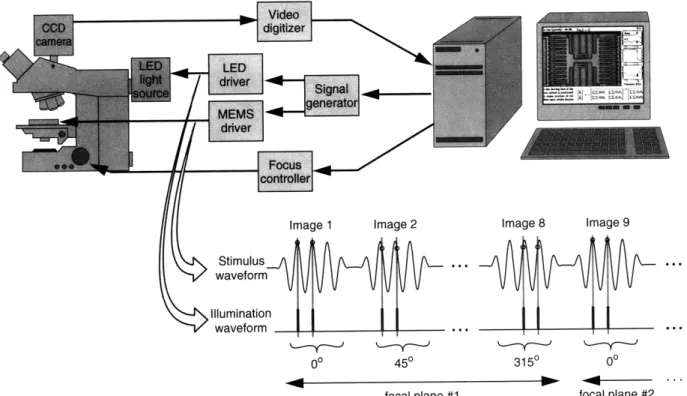
We are interested in developing tools for in situ mea-surement of micromechanical motions based on the combination of light microscopy, video imaging, and machine vision. MEMS are viewed with a microscope and imaged with a CCD camera while being driven with a periodic electrical signal (Figure 1). An LED is strobed once per stimulus period at a chosen phase, to yield a snapshot of the device position at the spec-ified phase. This process is repeated at several stim-ulus phases and at several focal planes. Computer vision algorithms estimate the change in position of the device between successive images. From these estimates, the periodic motion of the device is deter-mined. This process is repeated at other stimulus fre-quencies and/or amplitudes to characterize the device motion. Measured motions were decomposed into their predominant modes, and frequency responses of these modes were thereby obtained.
1.2 Calibration of Fatigue Test
Structures
Failure Analysis Associates, Inc., has developed test structures to investigate effects of stimulus and envi-ronmental conditions, as well as manufacturing pro-cess conditions, on the performance, aging, and ultimate failure of MEMS.1 The test structures consist of a proof mass that is rotated about its single point of attachment to the substrate (Figure 2, left panel). Motions are induced by electrical excitation of one comb drive and are sensed by the change in capaci-tance of the other comb. The goals are (1) to control
Chapter 1. Computer Microvision for Microelectromechanical Systems Video digitizer Image 1 Stimulus waveform Illumination waveform Image 2 450 focal plane #1
Figure 1. Computer microvision measurement system. The test device is placed on the stage of the microscope (left). A Pentium-based computer controls a signal generator that provides two synchrorized waveforms: one to drive motions of the test device and one to strobe the light source. Typical waveforms are
shown. Motions are driven with a sinusoidal stimulus. The first image is acquired when light from the LED samples the image at times corresponding to peaks in the stimulus waveform. Successive images are acquired at different phases. This process is then repeated for different focal planes selected by a computer-controlled focus adjustment.
environmental conditions, (2) to monitor changes in responses, and (3) to formulate quantitative models of reliability for MEMS.
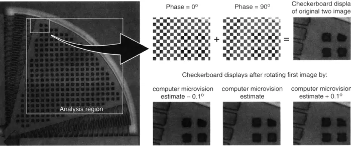
An important response property for development of quantitative reliability models is the angular displace-ment of the proof mass. We have applied computer microvision to obtain such measurements. Test struc-tures were excited with a variety of electrical stimuli and images were acquired and analyzed by com-puter microvision. To test that the rotation estimate between two images is qualitatively correct, the first image can be rotated by the estimated angular dis-placement and the resulting image can then be com-pared to the second. Such a qualitative analysis is shown in Figure 2 where registration errors are emphasized in a checkerboard display. Jaggedness
of the edges of structures in the checkerboard dis-play indicates registration error between the images. Although images are blurred by diffraction, they can be accurately registered to within a small fraction of the blurring radius using algorithms from machine vision. We use a gradient method that relates changes in brightnesses across images to gradients in brightness within an image. For example, if a pixel is illuminated by a middle part of a target that is brighter to the right and dimmer to the left, then the pixel should get brighter if the target moves to the left and dimmer if the target moves to the right. The gra-dient algorithm combines changes in brightnesses of all pixels in a region of interest (large white box in left panel of Figure 2) using a least squares method.2 Figure 3 show results of this algorithm for 5
indepen-1 S.B. Brown, W. Van Arsdell, and C.L. Muhlstein, "Materials Reliability in MEMS Devices." In Transducers '97, International
Confer-ence on Solid-State Sensors and Actuators, Chicago, Illinois, June 1997, pp. 591-93.
2 C.Q. Davis and D.M. Freeman, "Statistics of Subpixel Registration Algorithms Based on Spatio-Temporal Gradients or Block Match-ing," Opt. Eng., forthcoming; C.Q. Davis and D.M. Freeman, "Using a Light Microscope to Measure Motions with Nanometer Accu-racy," Opt. Eng., forthcoming.
Image 8 3150 Image 9 00 focal plane #2
.4-S1
Chapter 1. Computer Microvision for Microelectromechanical Systems
Phase = 900 Checkerboard display
of original two images
Checkerboard displays after rotating first image by: computer microvision computer microvision
estimate - 0.10 estimate
computer microvision estimate + 0.10
Figure 2. Accuracy of motion estimates using computer microvision. The left panel shows an image of a fatigue test structure designed by Failure Analysis Associates, Inc. One comb drive was stimulated sinusoidally at 20387.9 Hz to stimulate rotations at the mechanical resonance frequency of 40775.8 Hz. Images were acquired at 8 phases during each period of the electrical stimulus. Pixels in the analysis region indicated by the large white box were analyzed to determine the angular displacement. Portions from the upper right parts of the images taken at two phases were interleaved in a checkerboard fashion as shown in the upper right panel. The lower right panels illustrate similar checkerboard displays after the first image was rotated by the computer microvision estimate and by the estimate plus and minus 0.10.
1000 -100 -n 1 - 1- 01-Z = 0.1916 V 1.9 8 1 m-deg. I I t i l l I I I I I + + ++ ++ I 1I1111 I I I II 1 10 Stimulus amplitude V (p-p volts) 100
Figure 3. Calibration of fatigue test structure developed by Failure Analysis Associates, Inc. The device used in Figure 2 was stimulated at resonance with a sinusoidal voltage. Five independent
measurements (circles) were made at each of 15 different amplitudes (abscissa) of stimulation. The line given by the equation at the top of the plot is a regression line fit by a least squares method. Pluses indicate the standard deviations of results at each amplitude.
dent repetitions of the measurement at 15 different amplitudes of stimulation. The standard deviation for repeated trials is less than 4 milli-degrees p-p at all amplitudes.
1.3 Modal Analysis of the Draper
Gyroscope
The Charles S. Draper Laboratory has developed a microfabricated gyroscope for sensing angular veloc-ity.3
The gyroscope consists of two proof masses suspended by cantilevers. The masses are driven by comb drives along one axis so that angular rotation about the perpendicular in-plane axis induces a
cori-olis force in the out-of-plane direction. This force induces motion of the proof masses perpendicular to the substrate, and the motion is sensed as a change of capacitance between the proof mass and the sub-strate. The two masses are driven in opposite direc-tions to facilitate separation of angular velocity from linear acceleration.
The gyroscope is structurally complex and supports many modes of motion; the dominant modes of motion in the plane of the proof masses are a
tuning-3 J. Berstein, S. Cho, A.T. King, A. Kourepenis, P. Maciel, and M. Weinberg, "A Micromachined Comb-drive Tuning Fork Rate Gyro-scope," In Solid-State Sensor and Actuator Workshop (Cleveland, Ohio: Transducer Research Foundation, June 1993), pp. 143-48.
343
Chapter 1. Computer Microvision for Microelectromechanical Systems
fork mode (the difference mode of the two proof masses), and a hula mode (the common mode of the two proof masses). The hula mode can complicate the sensing of angular velocity by adding unwanted sensitivity to linear acceleration. Draper Labs has applied design and simulation tools to analyze undesired modes of motion. We have extended these efforts by experimentally measuring displace-ments of the proof masses and determining the con-tribution of in-plane modes of motion to these displacements.
Motions of the proof masses were measured using computer microvision under three stimulus condi-tions. In stimulus condition A, the outer combs of both proof masses were driven with a 40V p-p sinu-soid with 20V DC offset; this stimulus preferentially excites the tuning-fork mode. In stimulus condition B, the outer comb of the left-hand proof mass was driven; this stimulus preferentially excites the hula mode. In stimulus condition C, both combs of the left-hand proof mass were driven with the same voltage. This stimulus preferentially excites the out-of-plane levitation mode.
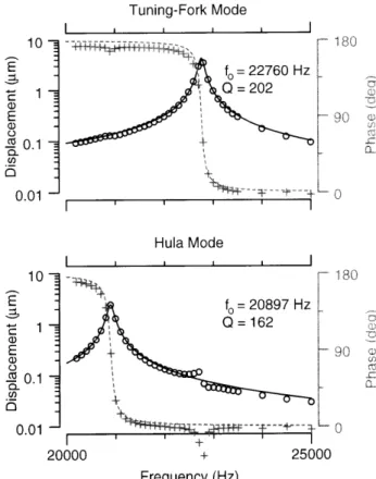
In all stimulus conditions, both tuning-fork and hula modes were induced. To estimate tuning properties of the tuning-fork mode, we computed half the differ-ence in motion of the two proof masses in stimulus condition A. To estimate tuning properties of the hula mode, we computed half the sum of the motions of the two proof masses in stimulus condition B. The magnitude of the frequency response of each mode was fit with a low-pass second-order resonance. Each fit had three free parameters-DC gain, reso-nant frequency, and quality of tuning (Q). The mea-sured and fitted phases were compared later to determine the goodness of the fit. Both modes were well fit by second-order resonances. The tuning-fork (difference mode) resonant frequency (in air) was 22.8 kHz with a Q of 202. The hula (common mode) resonant frequency was 20.9 kHz with a Q of 162. Figure 4 shows the measured modes and computed fits as a function of frequency.
Motions of any point on a structure can be described as a weighted sum of the dominant modes of motion of the structure.4 For example, in-plane motions of one proof mass of the gyroscope can be fit with a weighted sum of the tuning-fork and hula modes. The weights are the DC gains of the modes, which vary with stimulus condition and level and determine the contribution of each mode to the overall motion. The sum of the tuning-fork and hula modes gives a four-pole, two-zero system where the relative weights of the modes determine the locations of the zeroes, but not of the poles. The magnitude of motion of one proof mass was fit by this four-pole, two-zero system with two free parameters: one (gain) affecting the overall level of the fit, and one (relative mode weights) affecting the shape by changing the frequency of the zeroes. The fit was performed for the left proof mass under stimulus condition A, and for the right proof mass under stimulus condition C. As with the modal fits, a post hoc comparison of phase was done to determine the goodness of the fit. Motion of the proof masses under both stimulus con-ditions was well fit by the weighted sum of the modes. In stimulus condition A, the tuning-fork mode had a DC gain of 0.0525 tm, and the hula mode had a DC gain of 0.00277 rm. In stimulus condition C, the tuning-fork mode had a DC gain of 0.00604 gm, and the hula mode had a DC gain of 0.00101 gm. Figure 5 shows the measured displacements and computed fits as a function of frequency.
Chapter 1. Computer Microvision for Microelectromechanical Systems Tuning-Fork Mode II I I - = 6 f0= 22760 Hz o = 202 Hula Mode I , , , I I 44fFw Sfo= 20897 Hz
, +
,
20000 1~ 180 90 10-E 0 0 .1 Q.. 0o 101 -0.1 0.01Shuttle Displacement, Stimulus Condition A
I I I I
18(
-90
L0
Shuttle Displacement, Stimulus Condition C
I 1 1 1 1 1 1 I
- 180
+ 25000
Frequency (Hz)
Figure 4. Modes of motion of the Draper
gyroscope. Proof masses were driven by 40 V peak-to-peak sinusoid with 20 V DC offset. Displacements of both proof masses in the direction of excitation were measured at each frequency using computer
microvision. These displacements were subtracted and divided by two to estimate the tuning-fork
component, and were summed and halved to estimate the hula component. The modes were then fit with low-pass second-order resonances. The plots show the measured (symbols) and fitted (lines) magnitude (black circles) and phase (gray pluses) of the two modes. (a) Tuning-fork mode. This mode was preferentially excited by driving the outer combs of both proof masses (stimulus condition A).
Resonant frequency = 22760 Hz; damping coefficient = 0.00247; mean squared error = 1.13 nm. (b) Hula mode. This mode was preferentially excited by driving the outer comb of the left proof mass
(stimulus condition B). Resonant frequency = 20897 Hz; damping coefficient = 0.03085; mean squared error = 0.660 nm. 10-E a) 0.1 -C_ 0.01 -20000 180 25000 Frequency (Hz)
Figure 5. Modal reconstruction of proof mass displacement. Both plots show the displacement of a proof mass as a function of frequency. These displacements were fit with a weighted sum of the two modes shown in Figure 4. Symbols are as in
Figure 4. A. Displacement of the left proof mass, outer combs of both masses driven (stimulus condition A). The hula mode weight was 0.0528
relative to the tuning-fork mode. Mean squared error = 1.84 nm. B. Displacement of the right proof mass,
both combs of left proof mass driven (stimulus condition C). The hula mode weight was 0.1673
relative to the tuning-fork mode. Mean squared error = 0.243 nm.
1.4 Speckle Heterodyne Microscopy
We are developing a new method of light microscopy based on laser illumination. In a typical light micro-scope Figure 6, bottom panel), the light source is optically crude, providing approximately uniform illu-mination to the target. On the other hand, the micro-scope objective, the first and most critical element in the imaging chain, is optically sophisticated. There-fore, the optical quality of the objective is primarily responsible for the optical quality of the microscope. In speckle heterodyne microscopy, we adopt an alter-nate strategy: coupling highly precise illumination
345 0.01 -10 E a) -0 0.1 0.01 + 0
L
Chapter 1. Computer Microvision for Microelectromechanical Systems
from a laser source with a relatively crude detection system (Figure 6, top panel). Using beam-splitting and steering techniques, it is straightforward to gen-erate precisely structured illumination, such as high-spatial-frequency fringe patterns, that selectively excite features of the target. The key to resolution in the revised strategy is in the illuminator - not in the
detector. By substituting finely-patterned laser illumi-nation for high-precision lenses, speckle heterodyne microscopy will enable order-of-magnitude increases in both field of view and working distance. In addi-tion, in principle it can be implemented using micro-fabrication techniques. Thus speckle heterodyne microscopy holds potential to simultaneously improve performance and reduce costs of computer microvision systems.
Speckle Heterodyne Microscopy
coherent laser illumination shallow ~ angles cars Acoarse fringes steep angles fin fringes fringes low resolution detector
finely patterned illumination
Conventional microscopy
high
uniform precision high
resolution
illumination optics detector
detector Figure 6. Comparision of speckle heterdyne microscopy to conventional brightfield microscopy.
1.4.1 Publications Journal Articles
Davis, C.Q., and D.M. Freeman. "Statistics of Sub-pixel Registration Algorithms Based on Spatio-Temporal Gradients or Block Matching." Opt
Eng. Forthcoming.
Davis, C.Q., and D.M. Freeman. "Using a Light Microscope to Measure Motions with Nanometer Accuracy." Opt. Eng. Forthcoming.
Theses
Johnson, L. Using Videomicroscopy to Characterize
the Three-dimensional Motions of a Microfabri-cated Gyroscope. M.S. thesis, Department of
Electrical Engineering and Computer Science, MIT, June 1997.
Karu, Z.Z. Fast Subpixel Registration of 3-D Images. Ph.D. diss., Department of Electrical Engineering and Computer Science, MIT, September 1997.
1.5 Test Studies for
Microelectromechanical Systems
Sponsor
Defense Advanced Research Projects Agency Grant F30602-97-2-0106
Project Staff
Erik J. Pederson, Jared D. Cottrell, Michael B. Mcll-rath, Professor Donald E. Troxel
Microelectomechanical systems (MEMS) have the potential to revolutionize the design and production of sensors and actuators. However, the ultimate introduction of MEMS into major military and com-mercial systems depends critically on the speed with which MEMS can be designed and delivered into the field. The paucity of test equipment now available is an obstacle to the dissemination of MEMS for increasing the nation's defense and commercial competitiveness.
We call computer microvision the combination of light microscopy, video imaging, and machine vision. We are developing a series of MEMS stations to collect image data on various MEMS devices. The series of measurement stations will have a modular structure to enable the deployment of cost-effective measure-ment stations for the task at hand. A relatively more expensive MEMS station will have expanded specifi-cations. Our ultimate goal is to develop computer
Chapter 1. Computer Microvision for Microelectromechanical Systems
microvision as a useful tool for the design and manu-facture of MEMS-a tool that will enable the mea-surement of dynamical properties of the materials used to fabricate the MEMS device, as well as to characterize MEMS components used in larger sys-tems.
Work has begun to construct a MEMS station con-sisting of a PC, camera, probe station (including a microscope), stimulus generator, and strobe pulse generator. This system will provide pictures in order to analyze a candidate MEMS device. Considerable work has been done on the development of a strobe pulse generator to trigger a flash tube which illumi-nates the image to be captured. A novel technique for the generation of these pulses via a software algorithm has been proposed and will be evaluated and compared to the traditional approach using a phase-locked loop.