Any correspondence concerning this service should be sent
to the repository administrator:
[email protected]
This is an author’s version published in:
http://oatao.univ-toulouse.fr/24747
To cite this version: Garcia, Thierry and Spitéri, Pierre and
Khenniche, Ghania Behavior of parallel two-stage method for the
simulation of steel solidification in continuous casting. (2018)
Advances in Engineering Software, 131. 116-142. ISSN 0965-9978
Official URL
DOI :
https://doi.org/10.1016/j.advengsoft.2018.11.012
Open Archive Toulouse Archive Ouverte
OATAO is an open access repository that collects the work of Toulouse
researchers and makes it freely available over the web where possible
Research paper
Behavior of parallel two-stage method for the simulation of steel
solidification in continuous casting
T. Garcia
a, P. Spiteri
⁎,b, G. Khenniche
b,caIRIT-INPT, University of Toulouse, 2 rue Charles Camichel, B.P. 7122, Toulouse 31071 Cedex 7, France bIRIT-INPT-ENSEEIHT, University of Toulouse, 2 rue Charles Camichel, B.P. 7122, Toulouse 31071 Cedex 7, France cFaculty of Sciences, Department of Mathematics, Laboratory LAMAHIS, Skikda university, Algéria
Keywords:
Continuous casting Sparse non-linear systems Synchronous parallel algorithms Asynchronous parallel algorithms Multisplitting methods Two-stage methods
A B S T R A C T
This paper presents the behavior of general parallel synchronous and asynchronous multisplitting and two-stage methods for the numerical simulation of steel solidification in continuous casting. Thanks to the mathematical analysis and the implementation of these methods one can show the results of parallel experiments for the target application. The mathematical model is constituted by coupled nonlinear boundary value problems, namely the heat equation taking into account, on part of the boundary, a radiation phenomenon described by the Stefan law. For the numerical solution of such partial differential equations we consider, depending on whether the coef-ficient of thermal conductivity is constant or temperature-dependent, both an implicit or a semi-implicit dis-cretization with respect to the time of the studied evolution problem, while the spatial disdis-cretization is carried out by adapted finite difference schemes. Then large scale discretized algebraic systems are solved by sequential and synchronous or asynchronous iterative algorithms; comparison of these various previous methods im-plemented on clusters and grid are achieved in both cases when the thermal conductivity is constant and more generally dependent of the temperature.
1. Introduction and motivation
In steel industry, the continuous casting is a process between the
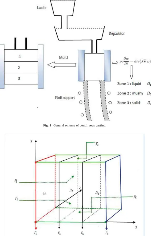
metal making and rolling. This process, shortly described inFig. 1,
al-lows the transformation of a liquid metal into a solid metal in a con-tinuous way. This casting can last as long as we can feed a repartitor by liquid steel; note that it is also possible to feed several parallel moulds. This industrial process is, by far, the most efficient for solidifying a great amount of metal. During the process the liquid metal is water cooled during the progress in the machine. As long as the steel pro-gresses into the machine, the solidified metal goes down at constant speed. Hence slabs or billets are obtained by the passage of liquid steel through several cooling zones. The transformation of the liquid phase into the solid phase takes place in an intermediary zone the so called mushy zone. To summarize the cooling solidification process, we can describe it in the following manner: the steel goes through three phases
in three areas denoted by Ω1for the liquid area, Ω2for the mushy area
and Ω3 for the solid area. The initial temperature in Ω1 is about
1500oC , while it remains equal to 800oC and 600oC , respectively in
Ω2and Ω3. This phenomenon describes a thermo-mechanical problem.
According to the previous description, we consider a steel portion in
the transverse direction of the continuous casting. The liquid steel poured into the mould cooled by water, after getting cold enough pe-netrates the cooling zones receiving optimal flow water quantity. This allows to take into account the primary and secondary cooling, in order to compute the thermal evolution of the steel. The temperature satisfies the heat equation with appropriate boundary conditions describing the physical phenomenon. During its development in the machine, the steel will be either cooled upon contact with the mould, either by the water jet or simultaneously with both. To describe this operation, it is as-sumed that the exchange of heat in the mould is uniform and the water jet cooling and thermal contact with the rollers constituted by cylinders will be modeled by the condition of convection and / or radiation. It is customary to assume that the contact surfaces with the ambient air are subject to conditions of the same type. The heat exchange that occurs between the subdomains liquid-mushy and mushy-solid is modeled by a condition at the interfaces. Every cooling zone is characterised by its temperature i.e, we have to find successively the temperature field in
the liquid zone Ω1, then in the mushy zone Ω2and finally in the solid
zone Ω3. For more details the reader is referred to Refs.[1–4].
The mathematical model used is based on the conservation of en-ergy resulting in the equation of diffusion of heat in three dimensional
⁎
Corresponding author.
E-mail addresses:[email protected](T. Garcia),[email protected](P. Spiteri). https://doi.org/10.1016/j.advengsoft.2018.11.012
space. The solution of this equation requires the knowledge of initial condition and six boundary conditions for each subdomain
=
, 1, 2, 3(seeFig. 2).
The solidification of steel in continuous casting is well described by considering the previous boundary value problems equipped with non-homogeneous linear and nonlinear mixed Dirichlet–Neumann and Fourier linear and nonlinear boundary conditions. Indeed for the con-tinuous casting problem, due to radiation phenomenon, well described
by the Stefan law on some parts of the boundaries, the linear part of the continuous operator modeling the heat diffusion is perturbed by a di-agonal increasing non-linear continuous operator, this last property resulting from the positivity of the temperature in each area. Nevertheless note that the positivity of the temperature in each zone
=
, 1, 2, 3is not obvious to prove; then we consider this positivity
as an assumption and the mathematical model is then changed as three coupled variational inequalities defined in three convex sets.
Fig. 1. General scheme of continuous casting.
,
find the temperatureu , =1, 2, 3,in each subdomain of the boundary
value problems governing the temperature. Besides taking into account both the constraint of temperature positivity and the nonlinearity de-rived from the radiation phenomenon are not convenient for the ana-lysis of the resolution algorithms. The more convenient formulation of these nonlinearities is constituted by a multivalued formulation of the problem, obtained by a perturbation of the continuous operators arising in the physical model by a diagonal multivalued monotone continuous operator; this last operator is in fact the subdifferential of the indicator function of the convex sets taking account of the positivity of the
temperature; for more details the reader is referred to Ref.[5]. After
discretization at each time, on one hand of the evolution part of the problems by an implicit time marching scheme when the thermal conductivity coefficient is constant or by a semi-implicit time marching scheme otherwise, respectively, and on the other hand by using clas-sical or adapted finite difference scheme for the spatial discretization with an uniform mesh, respectively, we have to solve, by a numerical way, a sequence of stationary multivalued nonlinear problems. So, fi-nally, at each time step, we have to solve three sparse large coupled strongly nonlinear systems.
Owing to the great size of such system, due to the difficulty of storage of large matrices, an iterative algorithm is more appropriate for the solution of the algebraic systems to solve and may be used in order to reduce the computation time at each time step. In the sequential context, we have implemented sequential projected point Newton -relaxation algorithms, corresponding to a coupling of the projected point Newton method for points belonging to the part of the boundary where the Stefan law occurs, with the projected relaxation method, like the point Gauss–Seidel method, for the interior points of the zones.
Besides, in order to obtain accurate results, it is necessary to choose very small spatial discretization step-size, which consequently leads to solve very large multivalued algebraic systems; such numerical solution is then time consuming. Thus, in order to reduce the elapsed time and taking into account the properties of the discretization matrices on one hand and, due to the positivity of the temperature on each zone
=
, 1, 2, 3, those of monotony for the nonlinear discretized
op-erators modeling the Stefan law on some parts of the boundary and also the well-known monotony of the subdifferential of the indicator func-tion of the convex sets on the other hand, we can state sufficient con-ditions for the convergence of the considered parallel synchronous and asynchronous multisplitting and two-stage methods for the solution of multivalued nonlinear algebraic systems in a general topological
con-text extending the initial results of[6]to the case where the finite
di-mensional space is normed by nonhilbertian norms more convenient to use. Note that such kind of methods, based on multisplitting method, allows a unified presentation and analysis of classical subdomain methods obtained on one hand by considering nonoverlapping sub-domains and on the other hand by considering the implementation of the Schwartz alternating method; for more details the reader is referred
to Refs.[7–17]. Note that, in these previous works the algebraic systems
are singlevalued; nevertheless in the present study, taking into account the positivity constraint of the solution by the perturbation of a diag-onal multivalued continuous operator extends many previous works in
this case. Moreover the paper[6]is also extended to a nonhilbertian
context.
The present paper is organized as follows. InSection 2, we present
the mathematical model of the solidification of steel in continuous casting in both cases where the thermal conductivity coefficient is constant and when it is dependent of the temperature; this section continues with a brief presentation of a multivalued formulation of the problem taking into account the positivity constraints of the
tempera-ture; for more details see[5]. InSection 3, we present the tools allowing
the numerical solution, particularly the discretization of the linear and nonlinear continuous operator governing the heat diffusion and also the
numerical sequential and parallel methods used for the solution of large scale algebraic systems; particularly the general parallel synchronous and asynchronous multisplitting and two-stage methods are presented and analyzed for the solution of algebraic systems perturbed by in-creasing diagonal multivalued discretized operators in the non-hilbertian context. This section is followed by the presentation of the parallel implementation of the algorithms. In the next section we will present the results of sequential and parallel experiments. The last section is devoted to the presentation of a general conclusion. 2. Mathematical model
2.1. Physical formulation
Let Rd,d=3,be a bounded open domain with boundary
de-noted by ∂Ω. We consider that =
=1 3
such that
= , .For the target industrial application note that it
is sufficient to consider that Ω has a parallelepipedic shape; so let
x y z
x ( , , )
and for = 1, 2, 3, let
, ,2 ,3 ,2¯ ,3¯ where for = 1, 2, 3, ={0 y, z 1, x=0}, 1 = = < < = = < < z y x y z x { 0, 0 1, 1 3 3}; { 1, 0 1, 1 3 3}, ,2 ,3 = = < < = = < < z y x y z x { 1, 0 1, 1 3 3}; { 0, 0 1, 1 3 3 }. ,2¯ ,3¯
Remark 1. Note that clearly ,2 (respectively ,2¯) shows the front
(respectively backward) of Ω; similarly ,3(respectively ,3¯) represents
the upper side (respectively under side) of Ω. The symbols 2¯ and 3¯, are a
convenient notation to simply define borders , =2, 3,and allows a
unified notation of these; without this notation, the forthcoming
description of the mathematical model (1)–(3) would be more
complex to write.
Let also Γ4and Γ5be the interfaces between Ω1and Ω2on one hand,
and between Ω2and Ω3on the other hand; thus Γ4and Γ5are defined by
={0 y, z 1, x=1 = y z x=
3}, {0 , 1,
2 3}.
4 5
The last frontier delimiting the domain Ω is defined by
={0 y, z 1, x=1}.
6
Then we have to find successively the temperatureu ,solution in
each subdomain , =1, 2, 3of the following boundary value
pro-blems:
in the liquid zone Ω1
= × = = = = = c div u in t u x t u x I C on u on u on ( ) 0, [0, ] , ( , 0) ( ), . . , , ( ), , ( ), u t final u n imp u n u n 1 1 1 1 1 1 1,0 1 1 1 1 1 1 1 1 1 4 1 1 1 1 (1)
in the mushy zone Ω2
Consequently we have to solve successively three coupled strong
= × = = = = = c div u in t u x t u x I C u u on u on u on ( ) 0, [0, ] , ( , 0) ( ), . . , , ( ), , ( ), u t final u n u n 2 2 2 2 2 2 2,0 2 1| 4 2 2 2 2 2 2 2 5 2 4 2 2 (2)
and in the solid zone Ω3
= × = = = = = c div u in t u x t u x I C u u on u on u u on ( ) 0, [0, ] ( , 0) ( ), . . , , ( ), , u t final u n imp 3 3 3 3 3 3 3,0 3 2| 5 3 3 3 3 3 6 3 5 3 (3) where I.C. denotes the initial conditions, and
= + =
u h u u u u
( ) cv, ( ext) ( 4 ext4), 1, 2, 3, (4)
describe the radiation phenomenon, modeled by the Stefan law and for = 1, 2, = u R u u ( ) 1( cst).
The significance of the various parameters is given below: for
= 1, 2, 3,c is the specific heat capacity, is the metal density, hcv,
is the coefficient of exchange by convection,u is the temperature, Φimp
is the flux, uimpis the temperature imposed, uextis the temperature of
environment, ucstis the constant temperature defined at the interface Γ4
and Γ5 between two consecutive subdomains where the thermal
ex-change is performed, R is the thermal resistance, ξ is the emissivity, δ is
the constant of Stefan–Boltzman andn is the outward normal vector. In
the sequel, such physical coefficients are assumed to be constant.
In the previous physical model , =1, 2, 3is the thermal
con-ductivity coefficient which possibly depends of the temperature; in this
last situation where is not constant, after experimental measurement,
the thermal conductivity coefficient is approximated, at each time step
p, by a piecewise linear function given by p(u)=ap+b up p,where
up [up min, ,up max, ] (see Table1). Such an approximation can provide a
better accuracy for the numerical simulation.Table 1displays the
va-lues of the coefficient apandbp. We show, in Fig. 3, the piecewise
linear approximation of the thermal conductivity coefficient.
2.2. Multivalued formulation
Taking into account the physical reality of the continuous casting problems, we impose the realistic assumption that the temperature
=
u , 1, 2, 3is a nonnegative function; then we can write the
fol-lowing assumption =
u( , )x t 0, for 1, 2, 3; (5)
while the problems(1)–(3)are unconstrained, we consider now in what
follows constrained problems. In this case, we have to solve a PDE’s
inequality corresponding to an obstacle problem (see [5]). The
solutions of these previous problems are therefore characterized by various formulations. Moreover, we consider also the temporal
dis-cretization of such problems (1)–(3) by an implicit time marching
scheme if the conductivity coefficients are constant or by a semi-im-plicit time marching scheme if these last coefficients are dependent on
the temperature in each area. Let us denote byw ( ), forx =1, 2, 3
the solution of the stationary obstacle problems where according to
assumption(5)we have
=
w ( , )x t 0, for 1, 2, 3, (6)
and in both cases, in the problems(1)–(3), the discretization with
re-spect to the time, at each timetp 1+ =(p+1) t,is carried out classically
by + = + u t u u t O( t), 1, 2, 3. p 1 p (7) So, at each time step, we have to solve the following stationary
obstacle problems on each subdomain , =1, 2, 3
+ + = = = = div w w g w e w in div w w g w e w in on w on w on ( ) 0, 0, . . ( ( ) ) 0, . . , ( ), ( ), c t c t w n imp w n w n 1 1 1 1 1 1 1 1 1 1 1 1 1 1 1 1 1 1 1 1 1 4 1 1 1 1 1 1 1 (8) + + = = = = div w w g w e w in div w w g w e w in w w on w on w on ( ) 0, 0, . . ( ( ) ) 0, . . , ( ), ( ), c t c t w n w n 2 2 2 2 2 2 2 2 2 2 2 2 2 1| 4 2 2 2 2 2 2 2 5 2 2 2 2 4 2 2 (9) and + + = = = = div w w g w e w in div w w g w e w in w w on w on w w on ( ) 0, 0, . . ( ( ) ) 0, . . , ( ), , c t c t w n imp 3 3 3 3 3 3 3 3 3 3 3 3 3 2| 5 3 3 3 3 3 6 3 3 3 3 5 3 (10)
where, e.w. means everywhere, Δt is the step time,g = ct wprec,and
=
wprec, 1, 2, 3is given thanks to the result obtained at the previous
time step.
We will now consider a different formulation of the previous sta-tionary variational inequalities in which the notion of subdifferential mapping, recalled hereafter, will play a main role in the sequel for
taking into account the constraints(6)onw , =1, 2, 3and the
ne-cessary projection on the closed convex set , =1, 2, 3associated
to the constraint(6). Indeed, classically in convex optimization (see
[18,19]) the problem (8)–(10) can be formulated by a multivalued
problem in each subdomain , = 1, 2, 3,defined as follows, where
Table 1
Piecewise linear approximation of the thermal conductivity coefficient.
variable p(u)=ap+b up p, =1, 2, 3 u u [ p min, , p max, ] (ap,bp) Ω1 [1508, 1627]; [1418, 1508] (19.6240, 0.0134); (−85.7667, 0.0833) [1400, 1418]; [1000, 1400] (0.8889, 0.0222); (14.2000, 0.0130) Ω2 [800., 1000]; [700., 800.] (20.7000, 0.0065); (73.1000, −0.0590) Ω3 [400., 700.]; [300., 400.] (57.0000, −0.0360); (49.8000, -0.0180) [200., 300.]; [100., 200.] (57.0000, −0.0420); (53.4000, −0.0240) [0., 100.] (51.8000, −0.0080)
=
E , 1, 2, 3denote appropriate vector spaces:
in the liquid zone Ω1, we have to findw1 E1
+ + = = = div w w g w on w on w on ( ) ¯ ( ) 0 , , ( ), , ( ), c t w n imp w n w n 1 1 1 1 1 1 1 1 1 1 1 1 1 1 4 1 1 1 1 1 1 (11)
in the mushy zone Ω2, we have to find w2 E2
+ + = = = div w w g w w w on w on w on ( ) ¯ ( ) 0 , ( ), , ( ), c t w n w n 2 2 2 2 2 2 1| 4 2 2 2 2 2 2 2 5 2 2 2 4 2 2 (12)
in the solid zone Ω3, we have to find w3 E3
+ + = = = div w w g w w w on w on w w on ( ) ¯ ( ) 0 , ( ), , , c t w n imp 3 3 3 3 3 3 2| 5 3 3 3 3 3 6 3 3 3 5 3 (13)
where (w), =1, 2, 3,are the sub differentials of the indicator
functions of the convex subsets ,defined by
+ < > × v w v w w v E ( ) ( ) , E E , for every , (14) where < > × ,
E E denotes the pairing
1between
E and E the dual
space of E and where the indicator function of the convex subset
E for = 1, 2, 3, is given by, =
+
w w
( ) 0 if
otherwise
Remark 2. Taking into account the values of the temperature in each area then obviously it seems not reasonable to think just one time that the temperature can be negative. Consequently the temperature is intuitively positive and even strictly positive. But the positivity of the
temperature in each area , =1, 2, 3 is not obvious to prove
mathematically even if it is true physically; this last point must be proved rigorously, and in the considered application, it is not obvious. The maximum principle seems very hard to apply in this context due to dominant Neumann or Fourier boundary conditions, with on some parts non linear formulation due to the Stefan law. Moreover, we have also to take into account the coupling between the different area liquid, mushy and solid. Thus in this non standard formulation, even if we can consider in advance an analogous result to the one stated when we have Dirichlet boundary condition concerning the minimum and / or the maximum value of the temperature, due to the Neumann or Fourier boundary condition on some part of the boundary, we have no information on the value and also on the sign of the temperature. Consequently, the question to use the maximum principle to show the positivity of the temperature in each area is an open and very interesting problem. Thus, instead of using the maximum principle, we consider an additional assumption allowing to make complete the mathematical model of solidification of steel in continuous casting.
Particularly such property ensures that the mapping
=
w (w), 1, 2, 3, are diagonal increasing continuous
operators. Moreover, the multivalued formulation is of some interest only from a theoretical point of view, due to the fact that the sub-differential of the indicator function is a monotone mapping and classically to take into account the constraints arising in the
mathematical model (see [18–20]); from a practical point of view,
such formulation does not play any role in the implementation of the numerical algorithm, since we have simply to carry out a projection on the convex set defining the constraint to respect the positivity of the temperature. Thus, classically due to the perturbation of the diffusion operator by the sub-differential continuous operator of the indicator
function of the convex sets , =1, 2, 3, we have to solve a
multivalued problem; due both to the monotony of the sub-differential operator, combined to the fact that the mapping
=
w (w), 1, 2, 3, are diagonal increasing continuous
Fig. 3. Piecewise linear approximation of the thermal conductivity coefficient.
1i.e. a bilinear form, from a normed vector space ×
E E onto ℜ. Recall
= < = w w w w ( ( )) , if 0, ] , 0], if 0, 0, if , i i i i i
and the corresponding graph is presented in Fig. 4. Recall that the
subdifferential ( . )is a monotone continuous operator, in general
multivalued, fromE to E ; for more details the reader is referred to
Ref.[20]. Note that inFig. 4the graph of the subdifferential of is
effectively monotone. Note also that, thanks to assumption (6), the
graph of w (w )is also monotone (seeFig. 5).
3. Numerical solution. 3.1. Discretization.
In a general framework, and in order to properly model the physical aspects, we must distinguish two cases; firstly the case where the thermal conductivity coefficient is constant and secondly the case where it depends of the temperature. Note that, in both cases, the
discretization with respect to the time, at each timetp 1+ =(p+1) t,is
carried out classically by using the scheme(7).
In the first case, the evolution problems(1)–(3)are discretized at
each timetp=p t,by an implicit time marching scheme and the spatial
part of the linear operator describing the heat diffusion is approximated by using the classical seven points scheme with an uniform mesh h, the spatial discretization step-size. Such combined discretizations leads to
the solution of a multivalued algebraic system described in(16)below.
In the second case where the thermal conductivity coefficient is not
constant, for sake of simplicity, we consider the discretization with respect to the time by a semi-implicit time marching scheme; so, in order to take into account the variation of the thermal conductivity coefficient we will in the sequel establish spatial approximation
schemes (see[21]). We consider a spatial discretization of the domain
Ω with an uniform mesh h, where h denotes once again the spatial discretization step-size. For the spatial discretization of the linear
continuous operators arising in(1)-(3), it is necessary to take into
ac-count that the coefficient of conductivity can not be constant in the
domain , =1, 2, 3. In order to obtain an estimate of the truncation
error, assume the classical assumption u 4( );assume also that
t x u
( , , )is continuous. It should be noted that in order to define the
scheme of spatial discretization by finite difference, we ask for more regularity in the solution than it actually has; however, such an as-sumption is classic and allows to obtain discretization error estimates. The discretization scheme is carried out by taking the mean of two intermediate schemes, called in the sequel forward-backward scheme
and backward-forward scheme [21]. Let us consider first the
dis-cretization of
( )
x u
x for =y yjand =z zkfixed. In order to simplify
the notations, let us denote by u t( ,p x y zi, j, k)=ui j k
p , , and = t x y z u ( ,p i, j, k, i j k) . p i j k p , , , , • Forward-backward scheme + + + + + + + + + + + + + + + + + + + + + + x u x h u x u x h h u u h u u h h h u h h u h u h 1 ( ) 1 ( ) ( ) p x p ip j k i j k p i j kp i j k p i j k p i j k p i j k p i j k p i j k p i j k p i j k p i j k p i j k p i j k p i j k p ip j k i j k p 1 1, , 1, , 1 , , , , 1 1, , 1, , 1 , , 1 , , , , 1 1, , 1 , , 2 1, , 1 , , 2 1, , 2 , , 1 1, , 2 1, , 1 i
Note that the truncation error of the forward-backward scheme is ( ).h
• Backward-forward scheme + + + + + + + + + + + + + + + + + x u x h u x u x h h u u h u u h h h u h h u h u h 1 ( ) 1 ( ) ( ) p x p i j k p i j k p i j k p i j k p i j k p i j k p i j k p i j k p i j kp ip j k ip j k i j k p ip j k i j kp i j k p i j kp i j k p 1 , , , , 1 1, , 1, , 1 , , 1, , 1 , , 1 1, , , , 1 1, , 1 1, , 2 1, , 1 1, , 2 , , 2 , , 1 , , 2 1, , 1 i
Note also that the truncation error of the backward-forward scheme is
h
( ).
Then, the final discretization scheme is obtained by making the mean of the two previous schemes. Thus the second derivative with respect to x is then approximated by
+ + + + + + + + + x u x B u B u B u h ¯ ( ) p x p i j k p i j k p i j k p i j k p i j k p i j k p 1 1, , 1, , 1 , , , , 1 1, , 1, , 1 2 i (15) with
Fig. 4. Graph of the subdifferential of the function .
operators, and also to the properties of the discretization matrices
presented below in the following Section 3.1, the analysis of the
behavior of the general parallel relaxation algorithms is very easy and we will conclude in the sequel to the convergence of the considered numerical parallel iterative methods, well adapted to this kind of problem. Note that another analysis using the orthogonal projection operator does not work here due to the nonlinearity appearing in the model problem because of the radiation phenomenon modeled by Stefan’s law since the associated fixed point mapping is hard to define correctly in such situation. Finally note also that the formulation of the model problem by a problem where the solution is subject to some constraint is as difficult to solve as the use of the maximum principle.
In (11)–(13), the projection on the convex sets , = 1, 2, 3 being classically and formally formulated by the perturbation of the
continuous operators by a multivalued increasing diagonal
con-tinuous operator, so, in the sequel, we will mainly use these
multi-valued formulations (11)–(13) of the model problems in order to
ana-lyze the behavior of the iterative algorithms used for the solution of these problems. Note that for = 1, 2, 3, the ith component of the subdifferential is given by:
= + = + + + + = + + B h B h B h 1 2 ( ), ¯ 1 2 ( 2 ), 1 2 ( ), ip j k ip j k i j kp i j kp ip j k i j kp i j k p i j k p i j k p i j k p 1, , 2 1, , , , , , 2 1, , , , 1, , 1, , 2 , , 1, ,
where B¯i j kp, , represents the approximation of the second derivative with
respect to x. Note that, due to the fact that the truncation error of the forward-backward and of the backward-forward schemes are equal in absolute value, but with opposite signs, by making the mean of the two
previous schemes, then the truncation error of the final scheme is (h2).
Similarly the other second derivative with respect to y and z are
approximated in the same way. For = 1, 2, 3, let us denote by pthe
heptadiagonal spatial discretization matrix defined by
= + = + = + = + = + = + = + + + + + + + + + + + + + + + B h B h B h B h B h B h B h 1 2 ( ); 1 2 ( ); 1 2 ( ); 1 2 ( ); 1 2 ( ); 1 2 ( ); 1 2 ( 6 ). i j k p i j k p i j k p i j k p i j k p i j k p i j k p i j k p i j k p i j k p i j k p i j k p i j k p i j k p i j k p i j k p i j k p i j k p i j k p i j k p i j k p i j k p i j k p i j k p i j k p i j k p 1, , 2 1, , , , 1, , 2 1, , , , , 1, 2 , 1, , , , 1, 2 , 1, , , , , 1 2 , , 1 , , , , 1 2 , , 1 , , , , 2 1, , , 1, , , 1 , , 1, , , 1, , , 1
Finally, at each time step, using an implicit or a semi-implicit time marching scheme, depending on whether or not the thermal con-ductivity coefficient depends of temperature, we have to solve three
sparse strongly nonlinear systems where for = 1, 2, 3, the global
spatial discretization matrix p in each subdomain is defined by
= + = c t Id ( · ), 1, 2, 3. p p (16) For the continuous casting problem, the Stefan condition is also taken into account by the perturbation of the linear part of the
dis-cretized system by a diagonal increasing disdis-cretized operator ;since
U representing the values of the temperature in the area
=
, 1, 2, 3,is assumed to be nonnegative, then at each time step p,
we have to solve the following algebraic systems
+ + = + + + U U U G ( p ) p p ( ) 0, 1, 2, 3, K p 1 1 1 (17)
where for = 1, 2, 3, p (R ),the space of linear operator inR ,
are strictly diagonally dominant M-matrices, , =1, 2, 3,denotes
the dimension of the matrices p, +
Up 1 R is the value of U at time
step (p+1), +
U
( p 1) results from the discretization of the
sub-differential of the indicator function and G are derived
from the time marching scheme.
3.2. General information on the numerical algorithms used
As previously said, owing to the great size of such systems(17), due
to the propagation of rounding errors which can perhaps distort the numerical results, iterative algorithm is prefered and may be used in order to reduce the computation time at each time step. Moreover, since the matrices are sparse, using iterative methods leads to a low cost of storage.
For the numerical solution we distinguish in the sequel the se-quential and the parallel methods which will be presented in an unified way.
In the sequential context, we have implemented sequential point projected Newton-relaxation algorithms, corresponding to a coupling of the projected Newton method for the points belonging to the
bound-aries with the projected relaxation method, like the projected
Gauss-Seidel method, for the interior points of , =1, 2, 3in which the
grid points are numbered using the lexicographical ordering. Moreover, very small spatial discretization step-size, leads to obtain
very large and sparse algebraic systems like(17). Due to possible very
large computation times, elapsed time reduction can be obtained by considering the parallelization of the numerical algorithms used. We can consider synchronous or asynchronous numerical parallel methods. More precisely, in a parallel context, we are in the present study in a specific situation which can be summarized as follows: we have to consider a global iteration called “outer iteration”, resulting in a dis-tribution of subproblems between processors and a local iteration re-sulting from the numerical iterative solution of each subproblem en-trusted to it, specific to each processor. So, in our case, each subproblem entrusted to one processor, is solved by an iterative algo-rithm, e.g. a point projected Newton method for the point belonging to
Taking into account the properties of the matrices , =1, 2, 3,
on one hand and the monotony of the discretized operators K (U)
and (U), =1, 2, 3on the other hand, for both previous iterative
methods, we present an analyze of the behaviour of the sequential and parallel synchronous and asynchronous two-stage method applied to
the solution of(17).
3.3. Multisplitting method 3.3.1. Preliminaries
In the present section we consider the general following problem
+ +
U U U G
( ) K( ) 0, (18)
similar to the problem (17), in which Ψ is an increasing nonlinear
discretized diagonal operator describing the Stefan law on some part of
the boundaries, (R )is a strictly diagonally dominant M-matrix,
,denoting the dimension of the matrix ,U ∈ ℜℵ, (U)results
from the discretization of the subdifferential of the indicator function
of the convex set and G is derived from the time marching
scheme. For a given vector V, let us associate to problem(18)an
im-plicit fixed point mapping V → F(V), defined as follows
+ + + = =
G V U (U) K(U) U F V( ) , V E ,
(19) where
=
denotes a splitting of the matrix .In the sequel we recall the following
classical definition (see[22])
Definition 1. Let E=R and L E( ); the decomposition
= is called a splitting if is nonsingular. It is called a
convergent splitting if the spectral radius of 1 ,denoted in what
follows ( 1 ) satisfy
<
( 1 ) 1. A splitting
= is
called
(i) regular if 1 0and 0,
(ii) weak regular if 1 0and 1 0.
Remark 3. Clearly, a regular splitting is a weak regular splitting, but the converse is not true.
The following result will be very usefull in the sequel.
Lemma 1. Assume that is an M-matrix admitting a weak regular splitting
= ; then, there exists a strictly positive vector ϑ ∈ ℜℵ and a
scalar ν ∈ [0, 1] such that the following inequality holds
= .
1 (20)
Proof. being an M-matrix, so there exists a strictly positive vector ϑ
such that =r =( ) >0.Note that 1r 0.Moreover if
= r 0, 1 for all … k {1, , },such that = = r ( ) 0, i k i i 1 1 , so that all
lines of are null, in contradiction with the nonsingularity of .Thus
> r 0; 1 therefore > < ( ) 0 , 1 1
and, since is an M-matrix, there exist both a strictly positive vector ϑ
and a positive real number ν < 1 such that(20)is valid, which achieves
the proof. □
Thanks to the previous result, we have the following Proposition: Proposition 1. Let us assume that
is an M-matrix, (21)
U ( ) is an increasing discretized operator,U (22)
U K( ) is a multivalued monotone maximal discretized operator,U
(23)
then the fixed point mapping V → F(V), defined by(19)is contractive, with constant of contraction equal to ν. So there exists one and only one fixed point U*, also unique solution of the discretized problem(18).
Proof.For sake of generality we consider that the space E is normed by any not necessarily hilbertian norm; let us denote by < ., . > the
pairing between E and E⋆
its topological dual space; G U˜ ( ) being the
duality map, we have
= < > = =
G U˜ ( ) { ˜ ( )g U E | U g U, ˜ ( ) U and g˜ 1},
where ‖U‖ and g˜ denote the norms of U and ofg U˜ ( ) in E and E⋆
respectively. For a point decomposition of U, let | . | be the absolute
value in such that the previous definition can be written as follows
= < > = =
G u¯ ( ) { ¯ ( )g u | u g u, ¯ ( ) | | and | ¯|u g 1}.
In the sequel let us denote by ui and vi, for i=1,…, the
components of the vectors U and V; in the same way we shall denote
by mi, jand ni, jthe entries of matrices and .Considering any
=
U F V( )andU´ =F V( ´ )we can write
+ + = +
U ( )U ( )U V G, where ( )U ( )( ),U (24)
and similarly
+ + = +
U´ ( ´ )U ( ´ )U V´ G, where ( ´ )U ( )( ´ ),U (25)
which involve, by subtracting the two previous relations
+ + =
U U U U U U V V
( ´ ) ( ) ( ´ ) ( ) ( ´ ) ( ´ ).
By multiplying the previous system by g U˜ ( U´ ) G U˜ ( U´ ) we
obtain < + + > =< > U U U U U U g U U V V g U U ( ´ ) ( ) ( ´ ) ( ) ( ´ ), ˜ ( ´ ) ( ´ ), ˜ ( ´ ) .
Consider now the ℵ following scalar equations resulting from the point
decomposition; due to assumptions (22) and (23) we have for all
…
i {1, , }
< i( )ui i( ´ ), ¯ (ui g ui i u´ )i > 0, and < i( )ui i( ´ ), ¯ (ui g ui i u´ )i > 0,
so that, we obtain the following inequality for alli {1, …, }
< + > < > = = mi i(ui u´ )i m (u u´ ), ¯ (g u u´ ) n (v v´ ), ¯ (g u u´ ) ; j j i i j j j i i i j i j j j i i i , 1 , 1 ,
since, on one hand
<(ui u´ ), ¯ (i g ui i u´ )i > =|ui u´ |i
and also, due to the fact that mi, j≤ 0 for i j
<mi j,(uj u´ ), ¯ (j g ui i u´ )i > mi j,|uj u´ |j
and on the other hand since classically <(vj v´ ), ¯ (j g ui i u´ )i > |vj v´ |,j
then finally we have
… = = m |u u´ | n |v v´ |, i {1, , }; j i i j j j i j j j 1 , 1 ,
the discretization points of and a point projected relaxation method for the interior points of , = 1, 2, 3; these iterative processes that are not necessarily carried out until its convergence, are called two-stage methods; for an algebraic linear system defined with an M-matrix [22] perturbed by a diagonal monotone discretized operator such al-gorithms have been analysed both for the synchronous and asynchro-nous case by several authors and the reader is referred to Refs. [6–17]. In the present work we extend the results of [6], stated in an hilbertian context, to the case where the finite dimensional spaces where the al-gebraic equations are defined, are normed by nonhilbertian norms, more convenient to use.
so, we obtain in a vectorial norm formulation
U U´ V V´ , V, ´V , (26)
which can still be written as follows =
U U´ 1 V V´ V V´ , V, ´V ;
Let us write componentwise this inequality = = = u u v v v v | i ´ |i | ´ | | ´ |, j i j j j j i j j j j j 1 , 1 ,
inequality that can be overestimated by = = u u V V V V | i ´ |i ´ ´ , j i j j i , 1 , ,
where ∥V∥ν, ϑ, is a uniform weighted norm defined by
= = … V max ( v ), i i i , 1, , (27)
with ν < 1, according to the result ofLemma 1. Therefore, we obtain
the following estimation
<
U U´ , V V´ , , V, V´ , 0 1. (28)
Then, using inequality(28), F is a contraction and we obtain a result of
existence and uniqueness of both the fixed point mapping of F and of
the solution of the discretized problem (18), which achieves the
proof. □
3.3.2. Parallel asynchronous method
In the present section, we recall the formulation of the parallel asynchronous method associated to the solution of the following fixed point problem
=
U E
U F U
Find such that
( ) (29)
where U F U( )is a mapping from D(F) ⊂ E to D(F). So, we consider
parallel algorithm, related to the natural block decomposition of the problem. For a general formulation of the algorithm, let α be a positive integer representing the number of blocks. In such algorithmic context
the space E is now a finite product of α subspaces Ei such that
= = E E . i i 1
Then let us consider the following block decomposition of U and F(U) = … U (U1,U2, ,U), and = … = … F U( ) F U( 1,U2, ,U) (F1(U),F2(U), ,F(U)).
In order to solve problem(29), let us consider now the iterative method
defined as follows: let U0∈D(F) ⊂ E be given, and then for all r
assume that we could getU1,…,Ur;Ur+1is recursively defined by
= … … +
(
)
U F U U U i s r U i s r , , , , if ( ) if ( ) i r i r j r r i r 1 1 ( ) j( ) ( ) 1 (30) where … … r s r s r i r i s r N N , ( ) {1, , } and ( ){1, 2, , }, the set { ( )} is infinite (31)
and for allj {1, …, }
= = r r r r r r j s r r N, ( ) N, 0 ( ) and ( ) if ( ) lim ( ) . j j j r j (32)
Note that = s r( ( ))r Nmodels the parallelism between the processors,
since s(r) contains the number of components relaxed at each step r
while =( ( ))r r Nmodels the asynchronism between the processors.
The choice of the relaxed components may be guided by any criterion; the more efficient criterion is then to pick-up the most recently avail-able values of the components just computed by the other processors.
The great interest of asynchronous parallel methods over synchro-nous ones lies in the fact that they eliminate processor latency when there are many unnecessary synchronizations, which causes periods of idle time of these latter. This situation is summarized in the following
Figs.6and7; inFig. 7 the grey area represents a phase of processor
inactivity.
Remark 4. Such asynchronous iterations describe various classes of parallel algorithms, such as parallel synchronous iterations if
…
j {1, , }, r , ( )r =r
j . In the synchronous context, for
particular choice of s(r), the previous fixed point method describes
classical sequential methods; indeed, if s r( )={1,…, }, i.e.
={ {1,…, },…{1,…, },…} then (30)–(32) describes the sequential
point Jacobi method while if s r( )=r mod. ( )+1, i.e.
={{1}, {2},…, { }, {1},…, { },…}then(30)–(32)models the sequential
point Gauss-Seidel method. In addition, if ={{1},…, { },
… …
{ }, { 1}, , {1}, {1}, , { }, { }, …,{1},…}then(30)–(32)models the
alternating direction method (ADI). We can now recall the classical result
Proposition 2. Let F: D(F) ⊂ E → D(F) and assume that
(i) = = D F( ) D F( ), i i 1
where Di(F) are closed and convex sets, (ii) there exists U⋆such that
=
U F U( ),
(iii) for all V ∈ D(F) we have F V( ) U , ¯
<
V U , ¯, 0 1, where here V , ¯ is the weighted uniform norm defined analogously to (27) but, here associated to the block
Fig. 6. Behavior of parallel asynchronous iterations.
decomposition and then given by = = … V max (v¯ ). i i i , ¯ 1, ,
Then every parallel asynchronous algorithm(30)–(32)associated with F and starting from U0∈D(F) converges to the fixed point U⋆of F.
Proof. Since F is a contraction the proof follows by a straitghforward
way from the application of a result of[23]. □
3.3.3. Parallel asynchronous multisplitting method
We consider now the solution of the problem (18) by parallel
asynchronous multisplitting method when satisfy assumption(21).
Let us also consider the m following regular splittings of
= l l, l=1,…,m m, N, (33)
where in what follows l are block diagonal, i.e.
=diag( ),i=1, …, ,l=1, …,m
l
i
l and moreover ( l) 1 0 and
0,
l corresponding to a regular splitting of . Let
= …
Fl: (Fl) (Fl), (Fl) E, l 1, ,m, be m corresponding fixed
point mappings associated with problem(18)and defined by:
= = …
Fl(V) U, l 1, ,m, U V, (Fl) E, (34)
by an analogous way than(24)and(25)and such that
= +
U V B;
l l
then, for all =l 1, …,m,the mapping Flassociated with problem(18)
are implicitly defined by
+ + + =
G lV lU (U) (U) U F(V) , V E.
K
l (35)
A formal multisplitting associated with problem(18)is defined by
the collection of fixed point problems (see[6])
= = …
U* Fl(U*), l 1, ,m, U* E. (36)
Let now consider the space = Emlike a finite product space of the m
spaces E defined by = = E , l m l 1
where El=E and consider the following m block-decomposition of
U˜ ,defined by = … … = U˜ {U, ,Ul, ,Um} E, l m l 1 1
whereU1, …,Ul,…,Umdenote m vectors of E.
Assume that the space is normed by the uniform weighted norm,
defined by a similar way to(27)by
= > = … = … V max ( max (|V| ( ¯ ))), ¯ 0, l m i i l l i l , ¯ 1, , 1, , (37)
where here |Vi| denotes any hilbertian or nonhilbertian norm of Viin
= …
Ei,i 1, , subspaces of E; assume that for =l 1, …,m, Fl are
con-tractive with respect to U*, its fixed point, with constant 0 ≤ νl< 1, so
that the following inequality is verified
= …
Fl( )V U* . V U* , for l 1, ,m.
l
, ¯ , ¯
l l l l (38)
Definition 2. The extended fixed point mapping : associated with the formal multisplitting is given as follows
= = = … = V U U F W V l m ( ˜ ) ˜ , such that l l( ), 1, , , k m lk k 1
where Wlkare nonnegative diagonal weighting matrices satisfying for
alll {1,…,m} = = W Id , k m lk l 1
Idlbeing the identity matrix in L(El).
Since Fl( (Fl)) (Fl),then obviously ( ( )) ( )where
= = F ( ) ( ). l m l 1
Note that considerable saving in computational work may be
pos-sible, since a component of Vkneeds not be computed if the
corre-sponding diagonal entry of the weighting matrices are zero; the role of such weighting matrices may be regarded as determining the distribu-tion of the computadistribu-tional work of the individual processors.
Let the following block-decomposition of the mapping
= … … = = V V V V E ( ) { ( ), , l( ), , m( )} . l m l 1 1
Note that for a particular choice of the weighting matrices Wlk, we
can obtain various iterative methods and particularly on one hand a subdomain method without overlapping and on the other hand the
classical Schwarz alternating method (see[6]). According with[6]the
block Jacobi method corresponds to the following choice of l
=diag I( ,…,I , ,I+,…,I ) ,
l
l l l l m
1 1 , 1
and to the choice of Wlk W¯lgiven by
= … …
W¯l diag(0, , 0,Il, 0, , 0),
which in other words means that the entries of the weighting matrices are equal to one or to zero.
For the additive Schwarz alternating method more than one pro-cessor computes updated values of the same component, and the
ma-trices Wlhave positive entries smaller than one.
Let us recall now a result of[6]
Proposition 3. Let us denote byU˜ *={U*,…,U*}where U* is the solution
of(18); then if assumption(38)is verified, is . , ¯ contractive with respect to U˜ *, where . , ¯ is defined by(37), the associated constant of contraction being
= max ( )<1.
l m l
1
Then, using the result ofProposition 3, we have the following result
Corollary 1. Consider the solution of problem(18); then if assumptions
(21)–(23)are verified, in particular if the matrix A is an M-matrix, then the formal multisplitting is contractive with respect to U˜ * and any sequential, parallel synchronous or asynchronous multisplitting method starting from U˜0 ( )converge to the solution of(18).
Proof. Indeed, if assumption (21) is verified, and if the other
assumption of Proposition 1 are satisfied then each fixed point
mapping Fl is contractive, for
= …
l 1, ,m and then the proof is
complete. □
Then, for =l 1,…,m,and for =i 1,…, ,such asynchronous
multi-splitting method can be given by
+ + = + = + + + = +
( (
)
)
U U U W V G i s r U U i s r ( ) ( ) , if ( ) if ( ), i l i l r i i l r i i l r l k m lk i k r i i l r i l r , 1 , 1 , 1 1 , ( ) , 1 , k where (U +) ( ) (U +) i i l r i i l r , 1 , 1Now, from the discretization of the solidification steel problem, we
have to solve, for = 1, 2, 3, the multivalued nonlinear algebraic
sys-tems(17). Each system(17)verifies all assumptions ofProposition 1 andCorollary 1. So we can conclude as follows
the matrix ;in such splittings for =l 1, …,m, lrefers as previously
said to a block diagonal matrix. Then we have α subproblems related
to the decomposition of lin α blocks. When the subsystems are solved
iteratively, we consider in addition the splitting of ldefined by
= , l=1, …,m,
l l l
where lare diagonal matrices. From an algorithmic point of view we
can perform a fixed number q of inner iterations or alternatively, under the previous appropriate assumptions, perform iterations until con-vergence. Using such new decomposition, we can define an asynchro-nous two-stage method as follows
+ + = + + + + + + + U U U U U G U U ( ) ( ) ˜ , ( ) ( )( ) l l r l r l r l l r l l l r l r , 1 , 1 , 1 , , 1 , 1 whereU˜l=
(
Ul r,…,Ul r)
. 1,1( ) , ( ) From a theoretical point of view, in the
sequel, let us also assume that for =l 1,…,m, l= l lis a weak
regular splitting while, as previously said, = l l is a regular
splitting.
Then , for =l 1,…,m,and for =i 1, …, ,such asynchronous
two-stage multisplitting method is given by
+ + = + + = + + + = + U U U U W V G i s r U U i s r ( ) ( ) ( ) , if ( ) if ( ), i l i l r i i l r i i l r l l r i l k m lk k r i i l r i l r , 1 , 1 , 1 , 1 , ( ) , 1 , k where (U +) ( ) (U +). i i l r i i l r , 1 , 1
In order to prove the convergence of the two-stage method, it is
necessary to state a similar result than the one obtained inLemma 1.
Lemma 2. Assume that is an M-matrix admitting a regular splitting
= ,where is a block diagonal matrix; moreover, assume also
that the matrix admits a weak regular splitting = . Let
= +
˜ 1( ).Then, there exists a strictly positive vector˜ R and
a scalar ˜ [0, 1]such that the following inequality
= +
˜ ˜ 1( ) ˜ ˜ ˜ (39)
is valid.
Proof. being an M-matrix, then the block diagonal matrix is
classically also an M-matrix, and 1 0.Besides, since is an
M-matrix, there exists a strictly positive vector ˜ such that
= = = >
r˜ ˜ ( ) ˜ ( ) ˜ 0.
Note that 1r˜ 0.Moreover if
= r˜ 0, 1 for all … k {1, , },such that = = r ( ) ˜ 0, i k i i 1 1
, so that all lines of are null, in contradiction with the
nonsingularity of . Thus 1r˜>0; therefore, by a straightforward
way, we obtain
> + <
( ) ˜ 0 ( ) ˜ ˜ ;
1 1
moreover since = is a weak regular splitting of , then
1 is a nonnegative matrix; furthermore since
= is a
regular splitting of then is nonnegative and 1is a nonnegative
matrix; it follows that 1 is also a nonnegative matrix and finally
is a weak regular splitting of ; since is an M-matrix,
there exist both a strictly positive vector ˜ and a positive real number <
˜ 1such that(39)is valid, which achieves the proof. □
So, similarly toCorollary 1, thanks to the result ofLemma 2which
ensures that the fixed point mapping associated to the two-stage method is contractive, we can conclude briefly on the convergence of the sequential and parallel synchronous and asynchronous two-stage methods applied to the model problem as follows.
Corollary 3. Consider the solution of the three constrained algebriac systems (17); then, since assumptions (21)–(23) are well verified, the sequential and parallel synchronous and asynchronous two-stage method starting from every initial guessU0converge to the solutionU*, =1, 2, 3,
of the problems.
4. Parallel implementation
In the present study the numerical solution of constant and variable coefficient models have been implemented in Fortran and use message passing programming on many independent computers, called nodes or processors. Due to their sparsity, the matrices are not globally stored. When using the finite difference method, in the first case where the coefficients of the diffusion equation are constant, it is sufficient to perform the calculation of the matrix coefficients only once at the be-gining of the numerical treatment. On the other hand, in the second case where the coefficients of the diffusion equation are not constant, due to the use of the semi-implicit scheme in selected time marching scheme, the matrix coefficients must be recalculated at each time step.
Then, in each subdomain seven subvectors are used in each
pro-cessor for the storage of the matrix. Thus for each subdomain we have to solve algebraic systems with about the same number of unknowns. During parallel process, we divide then this size of each algebraic system by the number of processors. We can then measure the interest of using an iterative method that does not require the storage of the whole matrix. Indeed considering its sparse character, this one is here represented in memory at most by seven subvectors that minimize memory occupation. Thus, using iterative methods allows clearly to minimize the storage memory. Each processor starts its own program and communicates with other nodes by sending and receiving mes-sages. Our parallel synchronous and asynchronous algorithms use the message-passing system called MPI (Message Passing Interface). MPI is a communication protocol which proposes for example point-to-point or collective communications and barrier synchronization. MPI can use TCP-based communications over IP interfaces. Our implementation is based on SPMD (single program, multiple data) paradigm, which is a commonly used approach for parallel and distributed applications. In SPMD, multiple autonomous processors simultaneously execute the same program with different data in order to obtain results faster.
Let n be the number of interior discretization points on each axis;
then we haven × n × n=n3 points on the complete domain Ω.
This domain Ω is split into 3 subdomains , =1, 2, 3with everyone
n/3 × n × n discretization points . In our case, for the parallel
si-mulation on α processors, each subdomain , =1, 2, 3is split into
subdomains ,j,j=1,…, with size about (n/3)/α × n × n points,
such that = ,
j j
, and the data are split accordingly into regular sets
and each processor initializes its own data set.
In the first case where the coefficients of thermal conductivity are constant, the matrix and the right hand side creation have been im-plemented sequentially since this part of computation is not very in-tensive. In other words, only intensive computations have been paral-lelized. In the case where the coefficients of thermal conductivity are not constant, then each processor is going to work with a part of the Corollary 2. Consider the solution of the constrained algebriac systems
(17); then, if assumptions (21)–(23)are verified, the sequential and parallel
synchronous and asynchronous multisplitting method starting from every
initial guess U0 converge to the solution U*, = 1, 2, 3, of the problems.
3.4. Two-stage multisplitting methods for pseudolinear problem
For pseudolinear problem such (18), we give in this section several particular classes of multisplitting methods called in the literature as two-stage methods; such two-stage methods corresponds to the fact that each subsystem is solved by an iterative relaxation method. Let us
as-l
norm of the difference between two successive updates. Finally, from a numerical behavior, due to the strong diagonal dominance of the ma-trices, the speed of convergence is high, so that in such situation two successive steps cannot be identical, and in this case, the numerical criterion used is robust. On the contrary when the speed of convergence is low, two successive steps could be slightly identical and far from the searched solution, which is not the case in the present study due to strong diagonal dominance induced by physical parameters as it will be seen in the numerical experiments.
So, for a current time step, when a local convergence is reached by a computing processor, a message is sent to the convergence manager processor; nevertheless, after such local convergence, the process con-tinues to iterate. Of course, if there is divergence after a convergence, a convergence cancellation message is sent. When the convergence manager processor detects the global convergence in all processors, it sends a stop message to computing processors.
This process is realized on each zone , =1, 2, 3 successively.
Then the next time step is performed for a given number of time steps
for all , =1, 2, 3. When all time steps are performed, the
compu-tation is ended; in this case, a final notification message is sent by one computing processors to the convergence manager processor. Note that the principle of the centralized stopping criterion is the same as well as for the synchronous algorithm than the asynchronous one.
Barrier synchronization. In order to use intrinsic MPI barrier
synchronization and to permit the independence of the convergence manager processor, we implement a synchronization barrier using broadcast function. In fact, it is the convergence manager processor which takes care of this barrier.
So, at the end of a time step, all the processors are synchronized thanks to this barrier and send a message to the convergence manager processor. Then this processor restarts each computing processor.
In a similar way, we use this synchronization barrier when the convergence is reached in all subdomains constituting one of the zone
=
, 1, 2, 3.
The algorithm of the convergence manager processor can be sum-marized as follows:
Algorithm convergence manager processor
receive command of processors
if barrier then
wait all computing processors
send notification restart to computing processors
else
if convergence then
receive local convergence
send global convergence
end if
end if
Parallel implementation without and with overlapping for the problem with constants coefficients and variable coefficients. The algorithms of the
numerical solution of constant coefficient model and variable coefficient model are identical except the compute of variable coefficients at each time step (see box below) and can be summarized as follows:
matrix and the associated right hand side, so they can be seen as a matrix and a vector filler that feeds a parallel linear system solver. This programming method greatly simplifies the solution of boundary value problems.
Two distinct parallel solutions are implemented by considering at each time step on one hand a subdomain method without overlapping and on the other hand a subdomain method with overlapping like the Schwarz alternating method; thus each zone , = 1, 2, 3 is divided into parallelepiped, each parallelepiped being identified by a pointer index system which refers to the number of points positioned on one of the axes and for the subdomain method with overlapping refers to the number of points considering the value of overlapping. Similarly, each
of the zones , = 1, 2, 3 is identified by a similar pointer index
system referencing either the first point or the last point of the zone on the same axis, respectively the first point minus the value of overlap or the last point plus the value of overlap of the zone on the same axis for the subdomain method with overlapping.
Firstly, the subdomain method with or without overlapping and also the synchronous or asynchronous method is chosen at the beginning of the solution. Then, each processor updates its assigned subblocks of components of the iterate vector. Thereafter, the transmission of the boundary blocks assigned to each processor to the contiguous blocks is realized.
Note that on each zone , = 1, 2, 3 a two-stage iterative method is implemented and note that the size of each subdomain is enough large in order to get to an efficient multiplicative behavior of the sub-domain method.
Stopping criterion. An efficient stopping criterion is implemented using a supplementary convergence manager processor devoted to this task. We prefer use another processor to avoid delays in communication between computing processors. We have used the stopping criterion proposed by Bahi et al. [24] based on the use of a centralized method.
The convergence manager processor centralizes the local con-vergences of all the computing processors. Every processor determines its local convergence; a local convergence corresponds to the fact that the uniform norm of the difference between two successive updates is
less than a given fixed threshold (see [25–27] for justifications). Note
that under assumptions similar to those considered in the submitted study that considering the norm of the difference between two suc-cessive steps provides convenient stopping criteria of iterations; note also, that in the three previous references, when considering such stopping criterion, we have stated some estimate of the value of cor-responding residue by using a property of approximate contraction induced by taking into account the propagation of round-off errors. In
r
fact, it was stated in Refs. [25–27], that each step r belongs to a set
r
centered at the fixed point solution U⋆, these sets being embedded
r
when the index r increases, so that when r tends to infinity, the sets tend to a limit set with small diameter. Indeed, in these previous re-ferences, both in the linear case (see [25,27]), when taking into account round off errors, and non-linear case [26], it is shown that this type of stopping criterion where the norm of two successive iterate vectors is considered is suitable; in addition, in these previous studies, when the convergence criterion is satisfied, an error estimate is drawn up which subsequently justifies the termination of iterations by considering the