THE COMMUNITY COSTS RESULTING FROM GROWTH
Robert Edward Coughlin A. B., Harvard College
1950
Submitted in Partial Fulfillment of the Requirements for the Degree of
Master in City Planning at
Massachusetts Institute of Technology
July 1955
7 Signature of Author
Certified by
ad, Department f City
and Regional Plannhig
July 27, 1954
Professor Frederiok J. Adams, Head, Department of City and Regional Planning School of Architecture and Planning Massachusetts Institute of Technology Cambridge 39, Massachusetts
Dear Sir:
In partial fulfillment of the requirements for the Degree of Master in City Planning, I submit
herewith this thesis entitled:
The Community Costs Resulting fram Growth. Respectfully,
ABSTRACT
This study of the community costs resulting from growth is an attempt to develop from the basic approach of Schussheim more general theoretical models relating several variables affecting the growth of towns and to treat their requirements for community facilitiesand services with more generalized cost data than has been applied in earlier studies. The models developed treat explicitly density and pattern of growth for residential development. They also provide for industrial and local commercial development. Space requirements, and requirements for municipal facilities are taken from planning and engineering standards and from current experience. The cost data for specific facilities and services are taken from the experience of many cities and towns, and are developed in the light of theoretical and engineering knowledge. Particular attempt is made to distinguish among levels of service
provided and to discover economies or diseconomies of scale in providing various municipal services.
Yearly costs are computed for several theoretical models for key years throughout the period of growth. All capital and operating costs incurred in the developing area are analyzed, but the analysis does not treat specifically the costs of facilities in the center of town which must be expanded because of the more intensive activity associated with the new growth. Nor does it treat the effect on community costs of the
existence of public facilities in the developing area which can serve the new growth.
Cost analysis of the theoretical models shows that density has a major effect on costs but its effect is not as great as that of the level of service provided. With the same complement and standard of service, low density growth always costs more than high density growth. However, at.low densities some services can be eliminated without harm to the town (e.g. public sanitary sewers). When these services are not provided, costs of low density development drop below costs for fully
serviced medium density developments. In all models, but especially in jump growth models, the cost per capita decreases as the development proceeds.
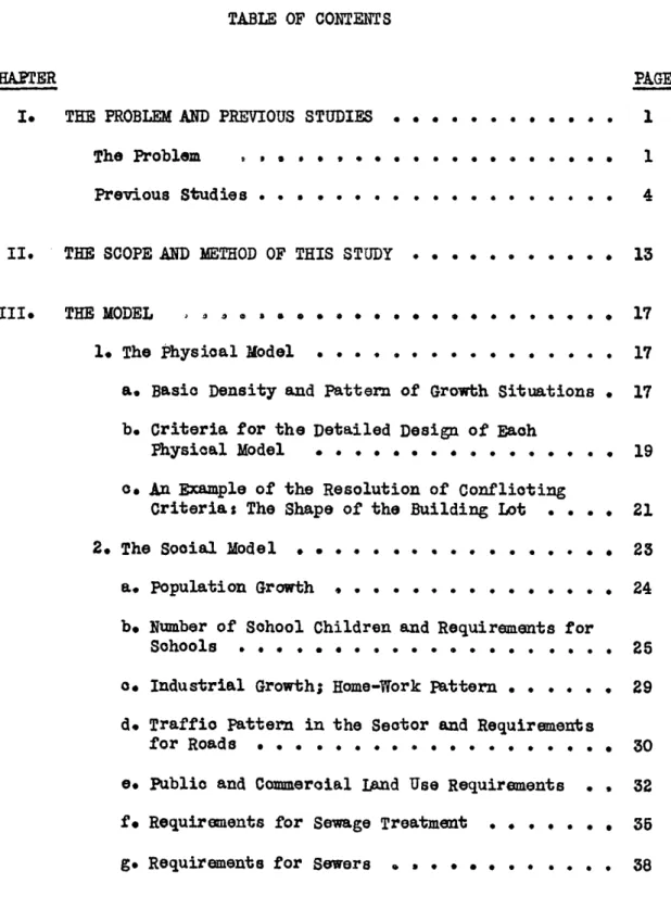
TABLE OF CONTENTS
CHASTER PAGE
I. THE PROBLEM AND PREVIOUS STUDIES ... 1 The Problem , .. . . .... . . ... . . . ... 1 Previous Studies . . . . . . . .* . . . 4 II. THE SCOPE AND METHOD OF THIS STUDY . . . . ... 13
III. THE MODEL 2 .. . . .. .... . .. . . . .. 17
l.
The Physical Model . . ... .. . . ... 17 a, Basic Density and Pattern of Growth Situations . 17 b. Criteria for the Detailed Design of EachPhysical Model . . . . .. . . . . . .. . . . 19 c. An Example of the Resolution of Conflicting
Criterias The Shape of the Building Lot . . . . 21
2.
The Sooial Model ... ... .. . .. . .. . 23a.
Population Growth * . . . . . . . . . . . . 24 b. Number of School Children and Requirements forSchools . . . . . . . . . . . . . . . . . . . . 25
c.
Industrial Growth; Home-Work Pattern . . . . . . 29 d. Traffio Pattern in the Sector and Requirementsfor Roads . . . .. . .. . . . . - . . . . . . 30 e. Public and Commercial Land Use Requirements . . 32 f. Requirements for Sewage Treatment . . . . . . . 35 g. Requirements for Sewers . .. ... . 38
PAGE
3.
Model Requirements Summary ..*
.. . . . .IV. THE COST DATA. . . . ... . . . .- - - . 1. General Considerations . . . . 2. Crudq Costs for Seiected Services: Public Welfare,
Police Protection, Health & Hospitals. General Government Control, Recreation, Libraries and General Public Buildings . . . . .
3.
Land Costs * ... *4.
Road Costs . e. . . . . a. Total Capital Costs . . . . .b.
Yearly Capital Costs . . . . o. Yearly Nonoapital Costs . . . . d. Roadway Costs Summary Chartse. Yearly Capital Costs for Curbs and 5. School Costs . . . . . . .
a. Total Capital Costs . . . .
Total Construction Cost . . . . Total Equipment Cost . .. . . . .
b. Yearly Capital Costs . . .. . .
. . . . * . - 0 e 0 0 . . . . .0 0 0 Sidewalks . . . .. 0.. .. .0 . .0 .0 .0 .0 .0 .0 .0 0 . 0 0 0 0 0
o. Yearly Nonoapital Costs for Secondary Schools. Expenditure and Quality of Education * * 0 0
d. Yearly Nonoapital Costs for Elementary Schools
e.
Size of School System and Efficiency . . . .f.
School Costs Summary . .* .. . .* . .0CHAPTER III. (Cont'd) 39 42 42 44 50 51 52 57 62 67 68 70 70 71 80 81 86 93 98 103 103
CHAPTER PAGE IV.
(Continued) 6. Sanitation Costs . . . . . . . . . . . . 105
a. Capital osts . . . . . . .. . . . .. . . .. * 105
Capital Cost of Sanitary Sewerage Treatment Plant . . . 105
Capital Cost of Sewer Lines. ... .. .. 107
b. Nonoapital Costs ... ... 109
7.Fire Proteotion Costs ... .. 111
V. THE COST ESTIMATES OF THE MODELS ... 114
1. Estimation of Total Yearly Costs . . . . . . 114
2. Cost Variation with Standard of Service.Provided . 115
3.
Cost Variation with Density . . . . . . . . . . . 1164.
CostVariation
with Pattern of Growth . . . . . . 1185. Cost per Dwelling Unit , . . .0 . . . 119
6. Community Costs When the Developer Bears the Primary Costs of Development *. . . . . . .. . . . 123
7. The Effect on Costs of Existing Unused Municipal Facilities . . . - . . . . . . . . 125
VI.
CONCLUSION . . . - . . . . . . .-. . . . . . . . . . . 128VII. APPENDIX I - Miscellaneous Tables .. . . . . . .. . . 132
HPTER PAGE III.
(Cont'd) APPENDIX III - Calculations of Yearly Costs for Medium Density Model, Continuous Development
Low Standard of Service. . . . . . . . . 142 APPENDIX IV - Detailed Summary of Yearly Costs of
Various Models ... . .. .. . 155 VIII. SELECTED BIBLIOGRAPMY .. ...
LIST OF TABLES
TABLE PAGE
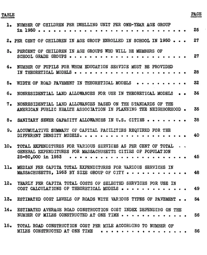
1. NUMBER OF CHILDREN PER DWELLING UNIT PER ONE-YEAR AGE GROUP
in 1950 . ... ... 25
2. PER CENT OF CHILDREN IN AGE GROUP ENROLLED IN SCHOOL IN 1950 . . . 27 3. PERCENT OF CHILDREN IN AGE GROUPS WHO WILL BE MEMBERS OF
SCHOOL GRADE GROUPS . . . . . *... . . . . . . .. . . . . 27
4. NUMBER OF PUPILS FOR WHOM EDUCATION SERVICE MUST BE PROVIDED
IN THEORETICAL MODELS . . . . . . . . . . . . . . . . . . . . . . 28
5. WIDTH OF ROAD PAVEMENT IN THEORETICAL MODELS . . ... e.. . . 32
6. NONRESIDENTIAL IAND ALLOWANCES FOR USE IN THEORETICAL MODELS . . 34 7. NONRESIDENTIAL LAND ALLOWANCES BASED ON THE STANDARDS OF THE
AMERICAN PUBLIC HEALTH ASSOCIATION IN PLANNING THE NEIGHBORHOOD . 35 8. SANITARY SEWER CAPACITY ALLOWANCES IN U.S. CITIES . . . . . . . . 38
9. ACCUMULATIVE SUMMARY OF CAPITAL FACILITIES REQUIRED FOR THE
DIFFERENT DENSITY MODELS ... 40
10. TOTAL EXPENDITURES FOR VARIOUS SERVICES AS PER CENT OF TOTAL GENERAL EXPENDITURES FOR MASSACHUSETTS CITIES OF POPUIAT ION
25-50,000 in 1953 . . . . . . . . . . . . . . . . . . . . . . . 45
11. MEDIAN PER CAPITA TOTAL EXPENDITURES FOR VARIOUS SERVICES IN
MASSACHUSETTS, 1953 BY SIZE GROUP OF CITY. . . . . . .. . . . . 48
12. YEARLY PER CAPITA TOTAL COSTS OF SELECTED SERVICES FOR USE IN
COST CALCULATIONS OF THEORETICAL MODELS . . . . . . . . . . . . . 49
13. ESTIMATED COST LEVELS OF ROADS WITH VARIOUS TYPES OF PAVEMENT . . 54 14. ESTIMATED AVERAGE ROAD CONSTRUCTION COST INDEX DEPENDING ON THE
NUMBER OF MILES CONSTRUCTED AT ONE TIME . . . . .. . . . . . . . 56
15. TOTAL ROAD CONSTRUCTION COST PER MILE ACCORDING TO NUMBER OF
LBLE PAGE 16. DEPRECIATION PER MILE OF ROADS HAVING VARIOUS TYPES OF
PAVEMENT . . . . . . . . . . . . . . . . . . . . 59
17. YEARLY DEPRECIATION PER MILE OF ROADS HAVING VARIOUS TYPES OF PAVEMENT ACCORDING TO THE NUMBER OF MILES CONSTRUCTED AT ONE
TIME .. . . . . .. .. . . . . .. . . . . .. . .. . 60 18. YEARLY .INTEREST COST PER MILE AT 2* PERCENT ACCORDING TO THE
NUMBER OF MILES CONSTRUCTED AT ONE TIME . . . 62 19. YEARLY ROAD MAINTENANCE COST PER MILE FOR VARIOUS TYPES OF
PAVEMENT . . . . . . . . . . . . . . . . . 63
20. ROAD MAINTENANCE COST INDEX ACCORDING TO NUMBER OF MILES TO
BE MAINTAINED . . . . . . . . . . . . . . . . . . . . . . .. 65
21. TOTAL YEARLY COSTS PER MILE FOR ROADS WITH VARIOUS TYPES OF
PAVEMENT
.
. * . . . * . . . . . . . . . 6722. YEARLY CAPITAL COSTS FOR CURBS AND SIDEWALKS.. . . . . .. . 69 23. TOTAL FLOOR AREA PER PUPIL FOR BUILDINGS OF VARIOUS LEVELS OF
SERVICE . . . 74 24. SCHOOL EQUIPMENT INDEX AREA INDEX AND CONSTRUCTION QUALITY
,INDEX ... .. ... ... ... 77 25. CAPITAL COSTS OF SCHOOLS PRESENTED BY SCHUSSHEIM IN
"RESIDENTIAL DEVELOPMENT AND MUNICIPAL COSTS" . . . . . . . . 78 26. COMPARISON OF PER PUPIL JUNIOR HIGH SCHOOL CAPITAL COSTS USED
IN SCHUSSHEIM'S STUDY WITH THOSE USED IN THIS STUDY . . . . . 79 27. CAPITAL COSTS PER SQUARE FOOT OF SECONDARY SCHOOLS ACCORDING
TO SIZE OF SCHOOL . . . . . . . . . . . . . . . . . . . . . .
84
28. CAPITAL COSTS PER SQUARE FOOT OF ELEMENTARY SCHOOLS ACCORDINGTO SIZE OF SCHOOL ... ... . . . ... . . * 85 29. ECONOMIES OF SCALE IN CURRENT COSTS OF SECONDARY SCHOOLS FROM
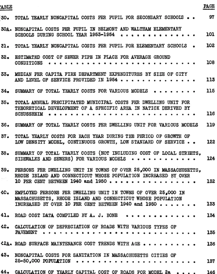
TABLE PAGE 30. TOTAL YEARLY NONCAPITAL COSTS PER PUPIL FOR SECONDARY SCHOOIS . . 97 30A. NONCAPITAL COSTS PER PUPIL IN BELMONT AND WALTHAM ELEMENTARY
SCHOOLS DURING SCHOOL YEAR 1953-1954 .. . . . . . . . 101 31. TOTAL YEARLY NONCAPITAL COSTS PER PUPIL FOR EIEMENTARY SCHOOLS . 102 32. ESTIMATED COST OF SEWER PIPE IN PLACE FOR AVERAGE GROUND
CONDITIONS # . . * s 8 * . . . . . . . . . . . . . . . . . .. 108
33. MEDIAN PER CAPITA FIRE DEPARTMENT EXPENDITURES BY SIZE OF CITY
AND LEVEL OF SERVICE PROVIDED IN 1954. *** . . . . 113
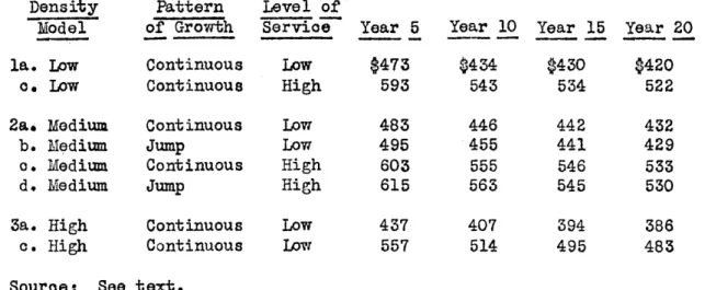
34. SUMMARY OF TOTAL YEARLY COSTS FOR VARIOUS MODELS . . . . . . . . 115 35. TOTAL ANNUAL PRECIPITATED MUNICIPAL COSTS PER DWELLING UNIT FOR
THEORETICAL DEVELOPMENT OF A SPECIFIC AREA IN NATICK DERIVED BY
SCHUSSBEIM . . . . . . . . . . . . . . . . - - . . . . . . . . . 116
36. SUMMARY OF TOTAL YEARLY COSTS PER DWELLING UNIT FOR VARIOUS MODELS 119 37. TOTAL YEARLY COSTS FOR EACH YEAR DURING THE PERIOD OF GROWTH OF
LOW DENSITY MODEL, CONTINUOUS GROWTH, LOW STANDARD OF SERVICE . . 122 38. SUMMARY OF TOTAL YEARLY COSTS (NOT INCLUDING COST OF LOCAL STREETS,
SIDEWALKS AND SEWERS) FOR VARIOUS MODELS . . ... . . . . 124 39. PERSONS PER DWELLING UNIT IN TOWNS OF OVER 25,000 IN MASSACHUSETTS,
RHODE ISLAND AND CONNECTICUT WHOSE POPUIATION INCREASED BY OVER
1OPER CENT BETWEEN 1940 and 1950. .. .. . . . .. . . . . .. 132
40. EMPLOYED PERSONS PER DWELLING UNIT IN TOWNS OF OVER 25,000 IN MASSACHUSETTS, RHODE ISLAND AND CONNECTICUT WHOSE POPULATION
INCREASED BY OVER 10 PER CENT BETWEEN 1940 and 1950 . . . . . . . 133 41. ROAD COST DATA COMPILED BY A. J. BONE . .. ... ... . 134
42. CALCULATION OF DEPRECIATION OF ROADS WITH VARIOUS TYPES OF
PAVEMENT . . .* . . . . . . . . . . . . . . . .. 135
42A. ROAD SURFACE MAINTENANCE COST TRENDS WITH AGE . . . . . . . . . . 136
43. NONCAPITAL COSTS FOR SANITATION IN MASSACHUSETTS CITIES OF
25-50,000
POPUIATION
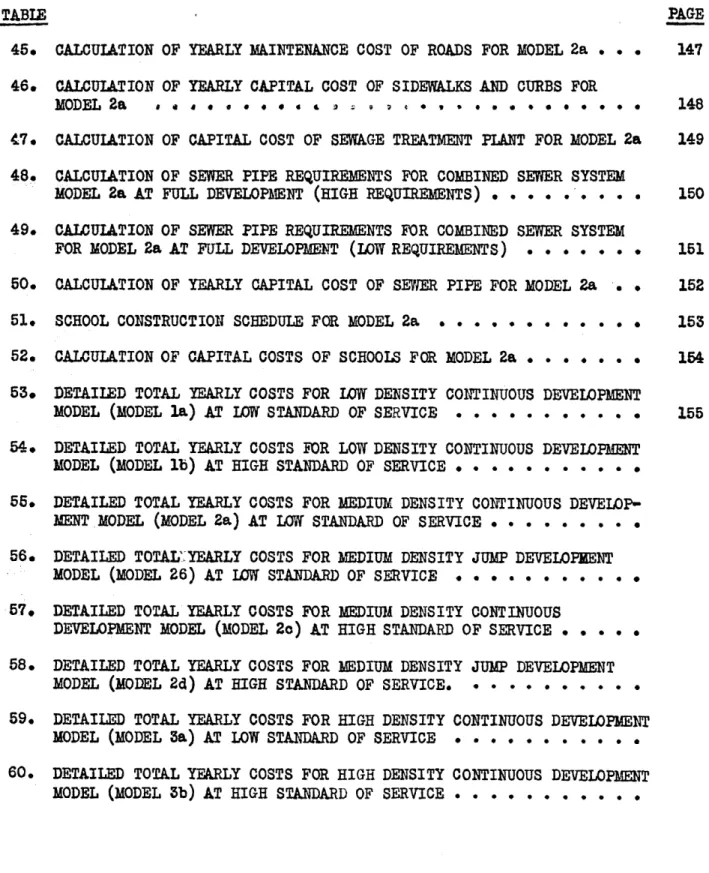
. . . . . . . . . . . . . . 137TABLE PAGE 45. CALCULATION OF YEARLY MAINTENANCE COST OF ROADS FOR MODEL 2a . . . 147 46. CALCULATION OF YEARLY CAPITAL COST OF SIDEWALKS AND CURBS FOR
MODEL 2a a t . * * . . . .. . * * . . . 148 47. CALCULATION OF CAPITAL COST OF SEWAGE TREATMENT PLANT FOR MODEL 2a 149 48. CALCULATION OF SEWER PIPE REQUIREMENTS FOR COMBINED SEWER SYSTEM
MODEL 2a AT FULL DEVELOPMENT (HIGH REQUIREMENTS) . . . . . . . . . 150
49. CALCUIATION OF SEWER PIPE REQUIREMENTS FOR COMBINED SEWER SYSTEM
FOR MODEL 2a AT FULL DEVELOPMENT (LOW REQUIREMENTS) . . . . . . . 151 50. CALCULATION OF YEARLY CAPITAL COST OF SENER PIPE FOR MODEL 2a . . 152 51. SCHOOL CONSTRUCTION SCHEDULE FOR MODEL 2a . . . . . . . . . . . . 153
52. CALCULATION OF CAPITAL COSTS OF SCHOOLS FOR MODEL 2a . . . . . . . 154 53. DETAILED TOTAL YEARLY COSTS FOR LOW DENSITY CONTINUOUS DEVELOPMENT
MODEL (MODEL la) AT LOW STANDARD OF SERVICE ... ... 155
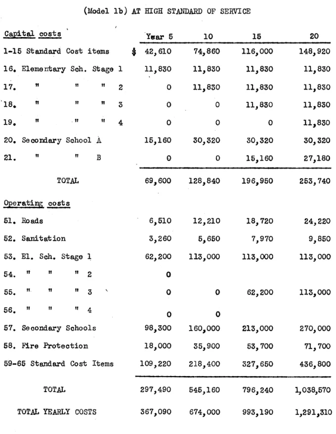
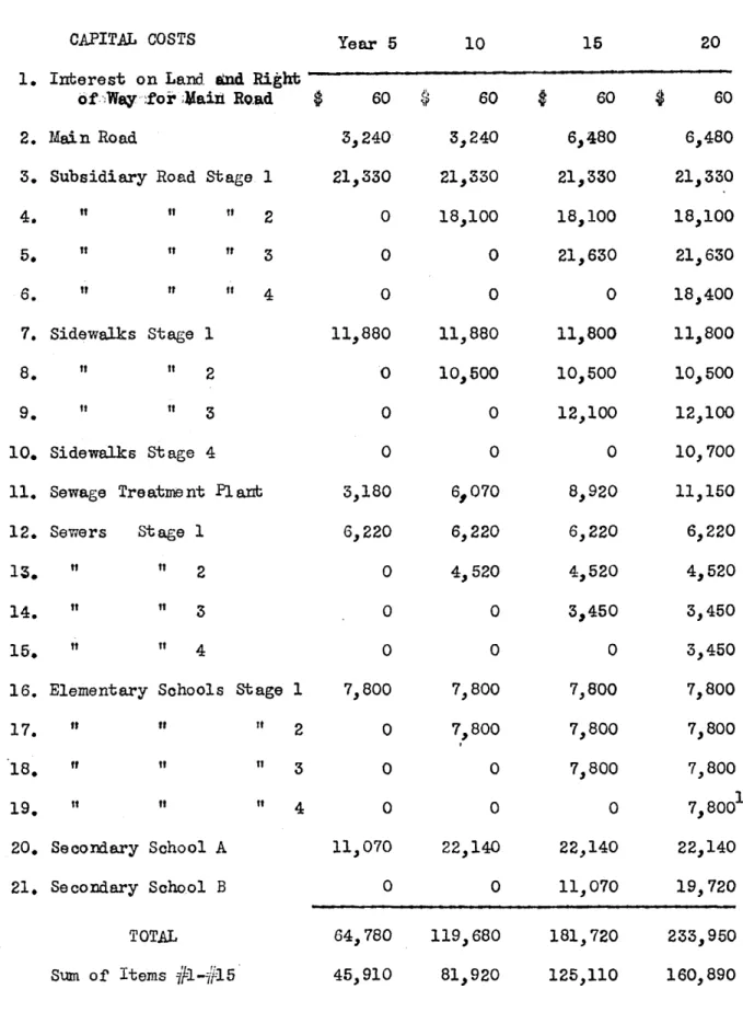
54. DETAILED TOTAL YEARLY COSTS FOR LOW DENSITY CONTINUOUS DEVELOPMENT MODEL (MODEL 1b) AT HIGH STANDARD OF SERVICE . . . . . . . . . . . 55. DETAILED TOTAL YEARLY COSTS FOR MEDIUM DENSITY CONTINUOUS
DEVELOP-MENT MODEL (MODEL 2a) AT LOW STANDARD OF SERVICE . . . . . . . . . 56. DETAILED TOTAL' YEARLY COSTS FOR MEDIUM DENSITY JUMP DEVELOPMENT
MODEL (MODEL 26) AT LOW STANDARD OF SERVICE ..
57. DETAILED TOTAL YEARLY COSTS FOR MEDIUM DENSITY CONTINUOUS
DEVELOPMENT MODEL (MODEL 2c) AT HIGH STANDARD OF SERVICE . . . . .
58. DETAILED TOTAL YEARLY COSTS FOR MEDIUM DENSITY JUMP DEVELOPMENT MODEL (MODEL 2d) AT HIGH STANDARD OF SERVICE. . .. . .. . . . . 59. DETAILED TOTAL YEARLY COSTS FOR HIGH DENSITY CONTINUOUS DEVELOPMENT
MODEL (MODEL 3a) AT LOW STANDARD OF SERVICE . . . . 60. DETAILED TOTAL YEARLY COSTS FOR HIGH DENSITY CONTINUOUS DEVELOPMENT
CHAPTER I
THE PROBLEM AND PREVIOUS STUDIES
The Problem
One continually hears municipal leaders make strongly voiced statements about the way in which a town can afford to grow. Some say, "Wfe cannot afford to spread out at low densities as some very rich sub-urbs do. It costs far more to provide roads, utilities and other munioi-pal services for low density developments than for high density developments." Others say, "We must have a large minimum lot size--one or two acres--for then houses will have a higher valuation and we will be able to collect enough taxes to pay for the education of the new children who come with the new houses. Our community will grow more slowly if we zone only for
large lot sizes because fewer people want to pay the extra money for large lots. Therefore, our needs for new capital outlay will be small." Some leaders have said, 'We don't want any industry in our town. It brings more expense than revenue. When industry comes, congestion increases. The town has to spend more for police and fire protection and utilities service for the industry. Along with industry come orkers who live in houses which cannot be valued highly enough to pay their way
in taxes. The rest of the town has to pay for the schooling of the workers' many children. Let some other tovm take the industry, we want a prosperous town of homes." Today more leaders are likely to say, "We must get industry in our town to strengthen its tax base. Tax revenue
2
from industry and commerce are necessary if we are to provide municipal services to our residents."
There is truth in each one of these statements, but no one of them tells the whole truth. For a particular town any one of these policies might be wisest. To decide which policy is best for a particular town,
one must consider the interrelations of many factors.
City planners, managers, and other officials can bring about many decisions that influence the type, location, amount and speed of growth. It is important that they understand the effect on community cost of the amount, density, location, and pattern of growth of new residential development. Is the difference in cost small enough that a certain type of development can be justified for noneconomic reasons even if the municipal costs associated with it are greater than for another less desirable type of development? What is the effect on community costs of the amount, location, and type of industry or other economic activity which develop within the town? How much do community costs change when various levels of service are provided by the municipality?
When growth of a community occurs, existing facilities and services are more intensively used in both the developing area and the older parts of the community. New capital outlays become necessary to serve the immediate needs of the new area and to serve the more intense activities in the old parts of town.
3
Some of the increased services can be provided by only small increases in the number of municipal employees. As the city grows it becomes less expensive to provide a unit of these services. In order to increase other services it becomes necessary to make sizeable capital outlays when growth overburdens existing facilities. New facilities cannot always be constructed to fit exactly the existing need. For example, a sewage treatment plant or a trunk sewer must be built all at once, not bit by bit each year. Often when they are first built, they are not fully utilized. As the community continues to grow, more and more people use the new facilities so the cost per unit of service
pro-vided decreases.
The community gets larger and the cost of a unit of service gen-erally becomes less, but at the same time more units of service per person may be needed. The increased concentration of activity in the community causes increased congestion. Better fire and police protection is needed, more elaborate roads are called for, increased recreation facilities are necessary, the general level of municipal service must be raised. To what extent increased economies of scale balance the
increased cost of higher levels of service is a complex and unresolved question.
Even if we could resolve all the intricacies of new costs pre-cipitated it would be premature to judge the economic feasibility of any development without studying the new revenues which also arise. With any
4
complex of urban costs due to growth there must be associated a complex of increased revenues. Increased tax revenue comes from the newly developed areas and also from commercial enterprises in the city which then operate more intensively and expand their plant to serve the new growth. Only when these new revenues as well as the new costs are estimated can we judge the effect of growth upon a city.1
Previous Studies
Few adequate sutdies have been made of urban costs and revenues. Most that have been made were not specifically concerned with the problems of growth, but with costs and revenues at some particular time. Little advance has been made from the case study level to a level of greater generality. As far as the author is aware, Schussheim's study of
municipal service costs precipitated by growth is by far the most incisive and complete study yet made. However, even it falls short of being a general study of the interrelations between costs, revenues, and growth. We lack a general framework within which analysis of the community costs
of growth can readily be carried out. This study is an attempt to develop a model which will recognize more of the interrelations than have been set
down previously.
1For an exploration of these new revenues and an analytic framework
which could be combined with that presented for new costs in this paper, see J. H. Larson, A Technique for Measuring the Effect of Industrial Growth on Municipal Revenue, unpublished Master's Thesis, M.I.T., 1955.
2
M. J. Schussheim, Residential Development and Municipal Service Costs: Case Studies in Three Communities in the Boston Metropolitan Area, unpublished Doctoral dissertation, Harvard University, 1952.
5
Perhaps one reason that good studies have been few is the difficulty of carrying out a valid cost analysis. Data exists on the expenditures of many towns, but an historical analysis of this data leads to many difficulties.
1. Over any period of time there have been significant changes in the prices of different types of goods and services. These price changes are bound to distort any analysis. Since these price changes vary
differently for different goods and services, they cannot adequately be compensated for by any cost index. A useful analysis must be based on present-day cost levels and relationships.
2. Change in the level of municipal service is almost inevitable over the history of any town, but it is extremely difficult to identify this variable in historical data.
3. In a town, many different types of growth in different areas are usually present. It is difficult to isolate the effects of one parti-cular growth. Since one cannot isolate the costs of a partiparti-cular growth
it is impossible to get the precipitated or marginal costs due to that growth. The analysis can only uncover average costs at any time.
It is not necessary to consider changes in prices and in level of service if costs and revenues of an area at any one time are analyzed. However, the resulting analysis throws light only on average costs and revenues, not on the specific costs and revenues which would arise from development of certain type and size in a particular location in the city.
6
One of the earliest cost-revenue studies was carried out by the Boston Planning Board in 1933 and 1934 /4/.1 It compared the cost of providing municipal services to particular residential sections, with the tax income from those areas. Costs were often apportioned arbitrarily. Varying percentages were allocated as general costs on the basis of assessed values, or as service rendered on basis of actual cases served, or by population. No notion can be gained of whether unit costs increase or decrease as the city grows. Capital costs for all purposes were
evidently all lumped together as City Debts; debts entered into by the city at many different times under many different price levels and for many different levels of. service are lumped together and simply allotted
to each tract by assessed value. There is no way to determine what new capital investments are required for the development of an area in a certain way. Municipal costs of new development are not likely to be the same as average costs of previous development. Both capital and current costs are treated as average costs; no light is thrown on marginal
costs.
Homer Hoyt has made several studies using this basic analysis
/8
and 9/. He treats only service costs, not capital costs for municipal plant. He has attempted more complex formulas for apportioning costs than were used in the Boston study. However, the simple approach of the Boston study often seems more acceptable than Hoyt's sophistication. For example, Hoyt states /t/ p. 24, "Apartment residents, having smaller1
A number enclosed in slant lines stands for the corresponding reference in the bibliography.
7
space for libraries at home, use library facilities much more intensively than single family residents." He therefore apportions library service costs; apartments, 60 per cent; single family homes, 35 per cent; other types, 5 per cent. When population in each type is considered, this shows that apartment dwellers use library facilities about 2.5 times as intensively as do single family home dwellers. In the same study /8/ p.34, in explaining how he allocated police service costs, Hoyt states,
"Because apartment areas occupy only one-seventh as much land area as single family home areas, and have six times as great a density, the cost of policing per dwelling unit is less for apartments than for single family homes. Instead of allocating the total cost to apartments on an area basis alone, an average of 14 per cent on area basis and 43 per cent on a proportion of total dwelling unit basis or 29 per cent (14 x 43
=
29)2 is used." These procedures have an element of logic behind than but that logic is not a rigorous basis for Hoyt's precise arithmetic.
Recently the Greenwich, Connecticut Planning and Zoning Commission /6/ has made a painstaking allocation of the costs of Greenwichts municipal government to classified property uses. Their procedure is more sensitive, but the scope of their study is similar to that of the Boston and Hoyt studies.
Had these studies even been unassailable in the logic of their cost apportioning they could not throw any light on the marginal costs of -new development or on the variation of these costs with density, pattern, and speed of growth.
8
A study of new capital costs caused by growth will throw light on these questions. New capital costs vary with the location, type, density,
size and pattern of new development. They also depend, to a large extent, on the unused capacity in existing municipal services and facilities.
In an outline of suggested research, William T. Ludlow /12/, p. 144, suggested that in order to understand how costs for newly developed areas vary with density and pattern of settlement, one should study the esti-mated public costs for various theoretical developments in various areas. Such theoretical developments should be similar in all respects except for variation in density and design. The estimated costs would be based on unit costs for various similar services and facilities in a specific city.
Such a study had been made of the cost of residential areas by Thomas Adams in 1934 /2/. This study indicated that in the low ranges of density much larger savings could be achieved by increasing density moderately than by increasing skill of design. By efficient design Adams could show only a 9.5 per cent reduction in the cost of public improvements for a development at a density of 6.5 dwelling units per gross acre. But when the density was increased to 10.25 dwelling units per gross acre, costs could be brought down by 54 per cent from the most expensive 6.5 acre development.
9
An important study carried out by F. Dodd McHugh /14/ in 1941 was
aimed at discovering the municipal costs of redeveloping urban areas. It considered the capital costs as well as the maintenance and operating costs of providing services for alternative types of developments of a 160-acre community. It then considered the effect on cost if the site were in different locations with respect to existing facilities which could be used by the new population. The study found that for one site total imporvement costs per capita declined as net density increased to 250 persons per net acre, then stayed constant until density reached 450 persons per acre, when it began to rise again. It would appear that for this very high density range characteristic of apartment areas of large central cities diseconomies are not encountered until extremely high densities are reached.
In the same study the public improvement cost per person of a development in Brooklyn, where no municipal facilities were available, was estimated by McHugh to be 340 per cent that of the same development in East Harlem, where many existing facilities could be used. In
McHughts study, capital cost data was taken directly from bids for similar work in New York. Current-costs data were taken directly from New York City operating agencies. The study made no attempt to discover any economies or diseconomies of scale, nor did it make explicit the yearly costs incurred due to amortization and interest on the capital cost of new facilities.
10
In a 1944 study for the Rye, New York Planning Commission, Frederick J. Adams /1/ estimated the cost of hypothetical residential development of varying type and density. However, the study did not consider the location of the development with respect to existing unused capacity in municipal facilities.
Ten years later, Morton Schussheim /18/ carried out a similar, but far more comprehensive study of hypothetical residential development in small and medium sized towns.1 This study specifically attacked the question of the municipal costs precipitated by growth. By case studies of three Massachusetts towns he showed the effect of density and size of development on capital costs and operating and maintenance costs.
1
Several other less exhaustive case studies have been made. The South East Pennsylvania Regional Planning Commission, in an unpublished study, has compared the municipal costs of the actual development of a specific area with what they might have been had the area been completely planned from the start.
An Analysis of the Probable Effects of the Extension of Levittown into MiMdletown TovishTp~ Bucks County, Pn~iEsyTvani /6/7con'siders new 'caita. and operating costs and concludes that the extension would cause Middletown residents little extra expense and the standard of several municipal services would improve.
The Institute of Public Service of the University of Connecticut 17/ has compared "the property tax yield of the small low cost home to its property tax cost."
/17/
p. 3. In this study (p.3) "the property tax costrofeassiall home . . .;is the net cost to the local property tax after deducting income from all other sources." The costs peculiar to a growing area are not considered.11
The study also considered the differentials of cost caused by the availa-bility of existing facilities in various locations. Three cases were considered:
1. A filling in of existing development.
2. Concentrated development in an area with some unused services. 3. Concentrated development in an area with few unused services. Schussheim separated public capital facilities into three groups and investigated the requirements of growth on each:
1. Primary facilities--capital inprovements that serve exclusively a new growth area (e.g. local streets and sewers).
2. Secondary direct facilities--facilities that have service districts wider than the growth area (e.g. trunk water and sewer mains, fire stations, elementary schools).
3. Secondary indirect facilities--town wide facilities used by old as well as new residents (e.g. junior and senior high school, water reservoir, central water pumping station, sewage disposal plant).
With his capital cost data organized this way he was able to show the effect on municipal costs of the current typical policy of requiring the developer to provide all primary facilities.
Unfortunately, it is difficult to generalize from Schussheim's results. He approached each town as a case study. Cost data for each town is different and was taken from the specific experience in each town. The availability of unused services is different for each location
12
of theoretical development. The level of service provided by each town is different. So many factors are different in his various theoretical developments that it is often most difficult to isolate the effect of a decision about density, pattern of growth, or level of service provided.1
Schussheim's framework could profitably be generalized to treat the impact of both residential and nonresidential development on a comnunity's cost structure.
1
The Di~sion of Planning of the Massachusetts Department of Commerce is now carrying out a promising study of "The Effect of Large Lots on Residential Development." They are studying in a general way the effect of lot size on (a) lot development costs, (b) municipal costs and income, and (c) metropolitan development.
CHAPTER II
THE SCOPE AND METHOD OF THIS STUDY
This study is an attempt to develop from Schuseheim's framework a more comprehensive method of analysing the community costs associated with new industrial development and population growth and to provide a
better understanding of the intricate interrelations of the various cost elements. The study treats theoretical models, but develops them with a large amount of cost deta from actual cities. Basic cost relations are
identified on a somewhat general basis so that they will be relevant for the study of a good number of communities. Several different general theoretical growth patterns are described. Then by the use of
theoretical knowledge, engineering computations, and sample data from a few actual developments, diverse community costs of new development are estimated. This is done for all direct costs and for as many indirect costs as are understood.
The analysis does not throw light on the cost of facilities in the center of town which must be enlarged to serve the intensified activity that will follow new growth. Neither does it treat explicitly the magnitude of cost advantage that will be enjoyed if development occurs
near existing facilities which can serve it. We consider the enlargeability of existing municipal plant and the availability of not completely utilized plant to be special conditions in any particular town which modify our
14
basic cost analysis. These conditions must be determined by a survey of the particular city in which growth is to be studied.
In the analysis undertaken, a first step is to identify some basic spatial dynamic growth patterns for towns under 100,000 population for a period of 10-20 years. We assume that residential values, behavior patterns, and technology (especially transport technology) will remain as we know them today and as they have been for the past five years. These patterns are intended to reflect rational behavior only. They are also typical patterns. These patterns relate to broad characteristics like the density of residential development and the extent of spatial continuity or discontinuity in growth. Other factors which influence the growth pattern are handled later in the analysis.
Theoretical physical models are designed for each of these patterns. Eaoh of these models provides for an increase of the same number of residences and the same number of acres of industry. The area and spatial distribution of the development differs in different density models. This is unlike the study of McHugh
/14/
which kept area constant. We conceive of the spatial extent and arrangement to be the result of an increase of residents and workers. We want to know what that growth costs; what are the low cost patterns, what are thehigh cost patterns and what variation there is in cost between the extremes. This approach makes it a bit more difficult to design the
15
physical models but leads to the simplification of many variables and makes it possible to relate cost to new population immediately.
Design of the physical layout is only one part of the design of the model. It is also necessary to construct a picture of the growing area's pattern of work places and how it is related to its town and
region. We must know the rate of residential and industrial development. We must know the special requirements of industry in the area and the
composition of the population. To the physical model is added the description of these relationships--the "social model." This complex model describes the physical facilities and services which the
community must provide for its development.
The study treats the growth of one spatial sector of a town only. An important future study would be to study the development of several
sectors at once or in sequence. Such a study would throw light on whether the costs of several sectors are simply additive or, because of the mutual interdependence of the various sectors, must be combined in some complex way. It could also investigate economies or diseconomies of operating at a much larger scale.
Cost of various municipal facilities and services are studied (roads, schools, police, fire, sanitation, etc.). Special attention is paid to distinguishing among levels of service and determining the extent of economies of scale in providing services. Cost data is derived from estimates of engin:ers, from theoretical analyses, and from actual costs
16
for comparable facilities and services. As much as possible, the resulting cost functions are presented as a set of charts.
The total yearly costs of public physical facilities and services called for by the model are computed for four key years spaced through the period of growth and the effects of variation in density, pattern of growth, and level of service are analyzed in turn.
CHAPTER III
THE MODEL
1. The Physical Model
a. The Basic Density and Pattern of Growth Situations
In order to study various possible general combinations of the density of residential development and the extent of spatial continuity or discontinuity in growth pattern, it was necessary to design several physical models.
All growth patterns can be thought of as a combination of three basic patterns of growth:
1. Spatially continuous concentrated growth outward from the existing town development.
2. Jump growth out from the town of a concen-trated development with a subsequent filling in
continuously back toward the original town. 3. Scattered grovith
a. Outside the existing developed area; b. Within the existing developed area.
It is very expensive to provide a given standard of municipal facilities and services to an area in which scattered growth occurs outside the existing developed area. Roads and utility lines must be extended long distances and are never fully utilized. Fire and police
17 P
protection must be spread thin. Either school busses or many small schools must be provided. By inspection, it appears that this pattern of growth will always be more expensive than any other. How much more expensive will depend on the degree of scatter. Since this pattern is inefficient from the point of view of municipal costs, we discount this pattern of development as irrational and inefficient and do not analyze
it further.
Scattered growth which fills in the existing developed area will probably be the least expensive pattern of growth because existing
facilities are likely to be available. Roads and sewer lines, fire stations and schools serve the existing population. Usually with only small
capital expansion these can serve the needs of the in-filling population. With this pattern of development, the unused capacity of existing facilities
and services is even more critical than usual. If large unused capacity exists, the public costs of development will be small indeed, but if roads must be widened, inadequate sewer lines replaced, and school sites
enlarged, costs will mount extremely rapidly. Under extreme circumstances the excessive cost of expanding such facilities could make the cost of this type of growth more expensive than any other. Since this study is not concerned with methods of estimating existing unused capacity or the
18
special costs of expanding and redeveloping public facilities, this pattern of development is not analyzed in detail.
If we eliminate analysis of scattered growth and consider the other two basic growth patterns and three densities, six possible basic physical models are theoretically necessary:
1. Continuous growth outward from the existing town development. a. Low density
b. Medium density c. High density.
2. Jump growth out from the town of a concentrated development with a subsequent filling-in back toward the original town.
a. Low density b. Medium density o. High density.
However, the physical model for jump growth is equivalent to that for continuous growth. The chief difference lies in the order in which different parts are developed. Therefore, we have but three basic physical models. These correspond to the three densities. We do not consider the high density-jump situation explicitly because due to the extremely short distances considered its physical development and resulting community costs are nearly equivalent to those of the high
density-continuous situation.
In order to examine all situations, jump-growth and continuous-growth models should be developed with respect to both industry and
19
residence. However, we are interested only in the more efficient spatial arrangements. It is believed most efficient to place all industry in one industrial estate. If this estate is placed as close as possible to the town, journey-to-work patterns, goods movement patterns and utility service lines are minimized, for by assumption our sector is on the
hinterland side of a town on the edge of a metropolitan sector. Therefore, in all models, we locate the industrial estate as close as possible to the already developed part of the town.
Diagrams of the three basic physical models are shown in figures
1-3. In our models low density refers to an average of one dwelling unit per not acre, medium density to four dwelling units per not acre, high
density to sixteen dwelling units per net acre. This range of densities is typical of present development in medium-sized towns.
b. Criteria for the Detailed Design of Each Physical Model. Several criteria were borne in mind for the design of the physical models:
1. The design should be as simple as possible in order that it may have as wide validity as possible and in order that it may permit the easiest calculations. Basic road patterns should change as little as possible in all models. (However, road spacing length and capacity does change with density.)
20
2. The same degree of design skill or ingenuity should be applied to each of the designs at different densities. Variations in cost due to the skill of the designer should be minimized.
3. A module or pattern should be created which can be repeated as
many times as the study requires.
4. The design should be rational and efficient, should provide all necessary facilities but no Iluxury" facilities. Cost should be minimized to the degree of best current practice. Cost savings are not to be
achieved at the expense of space standards commonly used by planners. 5. At the beginning of growth no excess capacity of any sort is available. At end of the growth considered no excess capacity should remain.
6. No unusual topographic or geological conditions are considered. We work with a "flat plain," uncomplicated by the random effects of
landscape. Only such variables as can be contolled by man (e.g. types and density of settlement, pattern of growth) are considered.
7. The design is conceived of as being executed in four stages--one every five years. Provision of special facilities should be apportistages--oned equally among the four stages, except when because of the logic of
development a facility must be built in the first stage or is definitely not needed until a certain later stage is reached. It is particularly important that the same facilities be assigned to the same stages in different density models unless the density of development definitely
dictates some different order of development. For example, a large playground around which roads and utilities must be extended should not be assigned to one stage, in one density model and to another stage in another density model.
To satisfy all these criteria is a difficult task. When, occasion-ally, demands conflicted it was necessary to work out compromises.
o. An Example of the Resolution of Conflicting Criteria: The Shape of the Building Lot.
The shape of building lot is a basic design element. Its choice required that two conflicting criteria be resolved. We want our design to be most efficient in its use of road and utilities. At the same time we must recognize planning standards for lot layout and shape.
It is well known that in a rectangular road system for any given acreage a square shape will minimize perimeter-road length. This indicates that the block should always be square, and, in fact, this is true as
long as one has access to the interior land of the block. To achieve access, there can be but two lots between roads in a rectangular road system. A square block of four square lots is the most efficient use of road if only four lots must be served. But if more than four lots are to be designed for, it is obviously a more efficient use of road to string lots together two lots deep and many lots long than to create several square blocks of four lots each. These long blocks of many lots become
22
more efficient users of road the more nearly square they are. They can be made to approach a square if the frontage of the individual lot is decreased and its depth increased. However, there is a minimum width which must be met to make a lot useful. One must choose between designing
the block which is the most efficient user of road and the lot which is of desirable shape. To compromise, we choose a lot of typical shape, with depth about twice its frontage.
In the low density (one dwelling unit per acre) model, we design a lot 150' x 290'. This means the local streets must be 580' apart.
I 5O
-
j I
I
In the medium density (four dwelling unit per acre) model, a lot is 75t x 145'. This means the local streets must be 290' apart.
23
In the high density (sixteen dwelling units per acre) model, individual lot size-loses meaning because most of the development will be in row houses or garden apartments. For simplicity, we develop our model with streets spaced 290' apart once more.
Diagrams of-the three basic physical models are shown in Figures 1-3. Their design could be undertaken only after we had posited the types, amounts and rates of growth expected. The next sections spell out this phase of our model building.
2. The Social Model
The requirements during the period of development for roads, schools, and sewerage cannot be determined until we have built up a "social model" which describes the amount and rate of residential and industrial growth, the expected number of children, and the expected traffic pattern.
In order to build up a model with which to work, we assume a set of "normal" requirements. These "normal" figures are simply estimates which fall within the range of experience and describe a norm. A
particular town could not be described entirely by this norm. To use our model to describe the cost of growth of a particular town it would be necessary to substitute the town's requirements which vary widely from our norm and which lead to major cost differences.
24
a. Population Growth
We conceive of a town of about 25,000 population on the edge of a metropolitan area. During the period of growth to be considered, it is
assumed that the town will approximately double in size. The theoretical sector in which growth is analyzed is conceived of as one of six radial sectors in the town. The population of this sector (sector X) will grow by nearly 8,000 people in 20 years.
We conceive of this twenty-year growth as the sector's ultimate growth. We neither plan for nor build facilities with capacity for any larger requirements. Implicit in our model building is the assumption that we foresee the complete development from the start. Therefore, we can
always plan, purchase, and build efficiently. We do not face the problem of replacing overburdened facilities ahd redeveloping areas to meet new conditions.
During the twenty years for which we analyze growth, we assume that: Sector X will increase by 2,480 dwelling units1 or by 7,940 people;
Sector A will increase by 2,480 dwelling units or by 7,940 people;
Sector B and C will increase by 1,650 dwelling units or by 5,280 people; Sector D and E will increase by 825 dwelLing units or by 2,640 people. Therefore, the total new population will be 23,800 people. We assume the central town remains at 25,000 people.
Hence in twenty years the total population will be 48,800. At the start sector X is undeveloped except for a poor secondary road which leads from the town through the area of sector X. We posit that sector X will develop at a constant rate as follows:
Year 5 Year 10 Year 15 Year 20 Barren except poor 620 DU 1240 DU 1860 DU 2480 DU secondary road 1980 persons 3970 persons 5950 persons 7940 pers
We assume 3.2 persons per dwelling unit. This is the median number of persons per dwelling unit in the seventeen towns of over 25,000 population in Massachusetts, Rhode Island, and Connecticut whose population increased by over 10 per cent between 1940 and 1950. See Table 39 in Appendix.
26
b. Number of School Children and the Requirements for Schools. For our purposes, the number of school children is the most important information concerning the composition of the population, for variation in the number of school children can cause significant
differences in public costs. In order to determine the characteristics of a growing population, we examined data on twenty-four cities in Massachusetts, New York, Connecticut, and Rhode Island whose population had grown by 10 per cent between 1940 and 1950. For each of these cities we calculated the number of children per dwelling unit in the elementary
school age group and the secondary school age group. We then calculated the average number of children per dwelling unit for each age by
dividing by the number of years in each school age group (see Table 1).
TABLE 1
NUMBER OF CHILDREN PER DWELLING UNIT
PER ONE-YEAR AGE GROUP IN 1950 Growth Cities Northeast
Average Average U.S. Average
7-13 Years old high .0550 median .0490 .0494 .0563 low .0435 14-17 Years Old high .0535 median .0430 .0440 .0494 low .0362
Source: Computed from statistics given in the County and City Data Book, 1952.
26
Little variation was noted between the average of "growth cities" and the Northeast average. (See Table 1.) The high U.S. Average may be partly because a larger percentage of rural families is found in the United States as a whole than in the Northeast or the growth cities.
The "7-13 years old" group shows more children per dwelling unit than does the older group. This reflects the recent rise in the nation's birth rate. Since we expect this birth rate to continue, we will make
our calculations of both grammar and high school population with the "7-13 years old" figures.
Not all children attend school. Some secondary school-age children especially are likely not to attend school. We examined the per cent of children in growth cities who were in school. It appears that compared with the Northeast and U. S. average a slightly higher per cent of the children in "growth" cities will be enrolled in school.
(See Table 2.) From the "growth" cities figures we interpolated the per cent attendance expected in each of the school-grade groups. (See Table 3.)
27
TABLE
a
PER CENT OF CHILDREN IN AGE GROUP ENROLLED IN SCHOOL IN 1950
Growth Cities 7-13 Years Old high median low 14-17 Years Old high median low 9705 96.5 90 95 88,3 80 Northeast Average 95.6 86.8 U.S. Average 95.7 83.7
Source: Computed from data given in the County and City Data Book, 1952.
TABLE 3
PER CENT OF CHILDREN IN AGE GROUPS WHO WILL BE MEMBERS OF SCHOOL-GRADE GROUPS
School Grade K 1 2 3 4 5 6 7 8 9 10 11 12 From "Growth Cities" Data 4---- 96.5- ---- 88.3
Estimate
Source: Interpolated from Growth Cities median 7-13 year.s old data of Table 2.
++--87----28
Our basic model shows an increase of 620 dwelling units every five years. We assume that public schools will provide all the service
required. If we assume a median number of children per dwelling unit, and apply our estimate of the per cent of children in each age group in
school (Table 3), then we find that school service must be provided for the following number of pupils:
TABLE 4
NUMBER OF PUPILS FOR WHOM EDUCATION SERVICE MUST BE PROVIDED IN THEORETICAL MODELS
Year 5 Year 10 Year 15 Year 20 Kindergarten and Elementary School 1 (K, Grades 1-6) 206 412 618 824 Secondary School (Grades 7-9) 86 172 258 342 (Grades 9-12) 79 158 237 316
Source: Computed from data of Tables 2 and 3 and population projection for model.
1
Examples of computations made to derive tablet;
We compute the number of children expected in grades 1-6: (620 D.U.) (0.0490 children per D.U. per one-year age group) (6) (98 per cent)
178 children.
We compute the number of children expected in kindergarten: (620 D.U.) (0.0490 children/DU/one-year age group) (1 year) (93 per cent)
=
28 children.29
The school requirements for these pupils are summarized in Table 9. In the high density model walking distances are short so only one large elementary school has been provided. In more spread-out models two elementary schools are provided.
a. Industrial Growth; Home-Work Patterns
In our model, industry is confined to a single industrial district. This minimizes goods transportation lines and is in line with the current recommendations of many town planners. If in our design we allow 17.61 workers per acre, the industrial district will cover 57 acres.
We assume that the industrial district will employs In 1960: 400 workers, of whom 100 will live in sector X In 1965: 600 " " " 180 " " t f " In 1970s 800 " " " 260 " t t " " In 1975: 1000 " " 35 " "t it
This allows for a slowly increasing percentage of total workers V& live in sector X. For each family living in sector X there are 1.4
workers,2 a total of 3,540 workers from sector X. We assume that those who do not work in the industrial district or in local shops find their
1
This figure is approximately the median number of employees per acre found in a survey of 220 plants made by the Urban Land Institute.
See Urban land Institute A4/, Table 20, p. 21).
2
This is the median number of workers per dwelling unit in the seventeen towns of over 25,000 population in Massachusetts, Rhode Island, and Connecticut whose population increased by over 10 per cent between
30
employment in the direction of the center of town. The metropolitan center can be reached from sector X only by going in the direction of the center of town.
Industry requires certain municipal facilities and services. Requirements for roads and sewage systems are the most important. They
are analyzed for both industrial and residential needs in sections d, f, and g following. Because of the limited time available we did not
analyze the need for police, fire protection, and other services which results from industrial growth. Instead, we make the crude assumption that these requirements can be projected on a constant per capita basis.
d. Traffic Pattern in the Sector and the Requirements for Roads. In order to be able to determine the highway needs of the sector, we must analyze the expected traffic pattern of the sector. How much traffic will sector X generate?
To answer this question, we have made several assumptions about the Journeys-to-work of the people who live in sector X. With these assumptions we have calculated the peak traffic expected on the main road. The assumptions and o&lcvlations are shown in Appendix II. Our calculations show that under the expected condition in year 20 at the intersection of the main road and the subsidiary road at the
industrial district, there will be a peak traffic load of 1,910 vehicles per hour.
31
Such a traffic load is too great for a two-lane highway but can be handled easily by a four-lane highway. In all models we have specified a main road with 44 foot pavement. This allows two ample lanes for traffic moving in each direction. Since the main road is a limited access parkway, no parking lanes have been provided. Traffic further out on the main road will be less, but rather than narrow the road to two lanes we have continued the 44 foot pavement.
If people living in the sector have a different pattern of work places than those outlined above, the resulting peak traffic pattern will be different. If we make different assumptions about where people work, will the amount of traffic vary widely enough to require different
highway capacity? The largest possible traffic load would occur if no one who lives in the sector works in the sector. Then all workers living in sector X would have to pass along the main road on their way to town. At the same time all the workers in the industrial district would have to pass along the same road as they come out from town. We analyzed this situation (see Appendix II, section 2) and found that the resulting maximum 2,500 vehicles per hour could be handled easily by the
same four-lane raod which was adequate for the "normal" home-work pattern.
1
The practical capacity of a 2-lane highway is 900 vehicles per hour under rural condition, 1,500 vehicles per hour under urban conditions. The practical capacity of a 4-lane road is 3,000 vehicles per hour under rural conditions and 4,500 vehicles per hour in urban areas. Three-lane roads are considered hazardous so we did not consider using one.
32
No traffic analysis was carried out for the subsidiary roads. We based their widths on current practice. (See Table 5.) In the low density models it is possible to provide narrower subsidiary roads than in the high density models. In low density residential areas parking as well as traffic is likely to be less intense per unit length of road. Note, for example,.that in the medium density model, local roads provide two-lanes for moving traffic and one lane for parking. In the high density model, it is necessary to provide an extra parking lane. In the low density model it is possible to eliminate the parking lane.
TABLE 5
WIDTH OF ROAD PAVEMENT IN THEORETICAL MODELS
Main Secondary Local
Road Road Road
Low Density 44' 24' 24'
Medium Density 44' 38' 30t
High Density 44' 44' 38'
e. Public and Commercial Land Use Requirements
The public and commercial land use allowances for our models are shown in Table 6. In positing nonresidential land requirements for our models we have allowed more land for these uses than do APHA /3/
minimum standards. Allowances based on APHA standards are presented in Table 7 in order that the reader may compare them with allowances for our model in Table 6.
We assume that commercial development will serve the primary needs of the residents and occasional needs of workers in the developing sector. More specialized needs will continue to be met by the existing shopping facilities in the center of town. We assume that one-half the ultimate required shopping facilities will be constructed during stage 2 of development; the other half will be constructed during stage 3 of development.
TABLE 6
NONRESIDENTIAL IAND ALLOWANCES FOR USE IN THEORETICAL MODELS
Low Density Model .l DU/A Medium Density Model 4 DU/A Number of High Density School
Model Children 16 DU/A (2480 DU) Elementary School
Junior High and High Schools Commercial Park Community Facili-ties Playground 1 4 0 4A 2@ 9A or 18A 1 @ 17A or 17A 2 Q 9A or 18A 1 @ 17A or 17A 7A 4A 46A 16A 62A 1 @ 18A or 18A 1 @ 17A or 17A 7A 10A 4A 56A 7A 6A 4A 52A
1In medium and high density models, it
is assumed that the school playgrounds are sufficent for sports which require large area like foot-ball and basefoot-ball. Four local p]aygrounds were provided in the low density model because with such spread-out development the distance from home to
elementary school playground is too great for the convenience of many children. The result is that the low density model, which already has the largest private areas, also ends up with the larges amount of land in public use. The low density model enjoys an inordinately high level of service in land use. However, since in our cost calculations we do not consider speoi-fically the development and maintenance of various public recreation lands, this high level of service is not reflected in our cost comparisons. We do not consider the purchase price of the land but assume that the subdivider deeds land to the community for public purposes. We see as a cost only the additional road and utility lines which must be constructed around the park.
824