COBRA IIIcMIT-2 : a digital computer program for steady state and transient thermal-hydraulic analysis of rod bundle nuclear fuel elements

TII

--

o:

EER.GY LBORATORY

JUL

)64

1981

MASSACHUSETTS INSTITUTE

OF

TECHNOLOGY

COBRA IIIc/MIT-2: A DIGITAL COMPUTER PROGRAM FOR STEADY STATE AND TRANSIENT THERMAL-HYDRAULIC

ANALYSIS OF ROD BUNDLE NUCLEAR FUEL ELEMENTS

by

J.W. Jackson and N.E. Todreas Energy Laboratory

and

Department of Nuclear Engineering

Massachusetts Institute of Technology Cambridge, Massachusetts 02139

Energy Laboratory Report No: MIT-EL 81-018 June, 1981

REPORTS IN REACTOR THERMAL HYDRAULICS RELATED TO THE MIT ENERGY LABORATORY ELECTRIC POWER PROGRAM

A. Topical Reports (For availability check Energy Laboratory Headquarters, Headquarters, Room E19-439, MIT, Cambridge,

Massacjhusetts, 02139)

A.1 General Applications

A.2 PWR Applications A.3 BWR Applications A.4 LMFBR Applications

A.1 J.E. Kelly, J. Loomis, L. Wolf, "LWR Core Thermal-Hydraulic

Analysis--Assessment and Comparison of the Range of Applicability of the Codes COBRA-IIIC/MIT and COBRA-IV-1," MIT Energy Laboratory Report MIT-EL 78-026, September 1978.

M.S. Kazimi and M. Massoud, "A Condensed Review of Nuclear Reactor Thermal-Hydraulic Computer Codes for Two-Phase Flow Analysis," MIT Energy Laboratory Report MIT-EL 79-018, February 1979.

J.E. Kelly and M.S. Kazimi, "Development and Testing of the Three Dimensional, Two-Fluid Code THERMIT for LWR Core and Subchannel Applications," MIT Energy Laboratory Report MIT-El 79-046.

J.N. Loomis and W.D. Hinkle, "Reactor Core Thermal-Hydraulic Analysis-Improvement and Application of the Code COBRA-IIIC/MIT," MIT Energy Laboratory Report No. MIT-EL 80-027, September 1980.

D.P. Griggs, A.F. Henry and M.S. Kazimi, "Development of a Three-Dimensional Two-Fluid Code with Transient Neutronic Feedback for LWR Applications," MIT-EL-81-013, April 1981.

J.E. Kelly, S.P. Kao and M.S. Kazimi, "THERMIT-2: A Two-Fluid Model for Light Water Reactor Subchannel Transient Analysis," MIT-EL-81-014 April 1981.

J.W. Jackson and N.E. Todreas, "COBRA IIIc/MIT-2: A Digital Computer Program for Steady State and Transient Thermal-Hydraulic Analysis of Rod Bundle Nuclear Fuel Elements," MIT-EL 81-018, June 1981.

A.2 P. Moreno, C. Chiu, R. Bowring, E. Khan, J. Liu, and N. Todre s,

"Methods for Steady-State Thermal/Hydraulic Analysis of PWR Cores," MIT Energy Laboratory Report No. MIT-EL 76-006, Rev. 1, July 19 7/J 27 1

(Orig. 3/77).

J. _{Liu, and N. Todreas, "Transient Thermal Analysis of PWR's aby a}

Single Pass Procedure Using a Simplified Model Layout," MIT Energy

Topical Reports (continued)

J. Liu, and N. Todreas, "The Comparison of Available Data on PWR

Assembly Thermal Behavior with Analytic Predictions," MIT Energy

Laboratory Report MIT-EL. 77-009, Final, February 1979, (Draft, June 1977).

A.3 L. Guillebaud, A. Levin, W. Boyd, A. Faya, and L. Wolf, "WOSUB-A

Subchannel Code for Steady-State and Transient Thermal-Hydraulic

Analysis of Boiling Water Reactor Fuel Bundles," Vol. II, Users Manual, MIT-EL 78-024, July 1977.

L. Wolf, A. Faya, A. Levin, W. Boyd. L. Guillebaud, "WOSUB-A Subchannel Code for Steady-State and Transient Thermal-Hydraulic Analysis of

Boiling Water Reactor Fuel Pin Bundles," Vol. III, Assessment and Comparison, MIT-EL-78-025, October 1977.

L. Wolf, A. Faya, A. Levin, L. Guillebaud, "WOSUB-A Subchannel Code for Steady-State Reactor Fuel Pin Bundles," Vol. I, Model Description, MIT-EL-78-023, September 1978.

A. Faya, L. Wolf and N. Todreas, "Development of a Method for BWR

Subchannel Analysis," MIT-EL-79-027, November 1979.

A. Faya, L. Wolf and N. Todreas, "CANAL User's Manual," MIT-EL-79-028,

November 1979.

A.4 W.D. Hinkle, "Water Tests for Determining Post-Voiding Behavior in the LMFBR," MIT Energy Laboratory Report MIT-EL-76-005, June 1976.

W.D. Hinkle, Ed., "LMFBR Safety and Sodium Boiling - A State of the Art Report," Draft DOE Report, June 1978.

M.R. Granziera, P. Griffith, W.D. Hinkle, M.S. Kazimi, A. Levin, M. Manahan, A. Schor, N. Todreas, G. Wilson, "Development of Computer Code for Multi-dimensional Analysis of Sodium Voiding in the LMFBR," Preliminary Draft Report, July 1979.

M. Granziera, P. Griffith, W. Hinkle (ed.), M. Kazimi, A. Levin, M. Manahan, A. Schor, N. Todreas, R. Vilim, G. Wilson, "Development of Computer Code Models for Analysis of Subassembly Voiding in the LMFBR," Interim Report of the MIT Sodium Boiling Project Covering Work

Through September 30, 1979, MIT-EL-80-005.

A. Levin and P. Griffith, "Development of a Model to Predict Flow Oscillations in Low-Flow Sodium Boiling," MIT-EL-80-006, April 1980.

M.R. Granziera and M. Kazimi, "A Two-Dimensional, Two-Fluid Model for Sodium Boiling in LMFBR Assemblies," MIT-EL-80-011, May 1980.

G. Wilson and M. Kazimi, "Development of Models for the Sodium Version

of the Two-Phase Three Dimensional Thermal Hydraulics Code THERMIT," MIT-EL-80-010, May 1980.

B. Papers

B.1 General Applications B.2 PWR Applications B.3 BWR Applications B.4 LMFBR Application

B.1 J.E. Kelly and M.S. Kazimi, "Development of the Two-Fluid Multi-Dimensional Code THERMIT.for LWR Analysis," Heat Transfer-Orlando 1980, AIChE Symposium Series 199, Vol. 76, August 1980.

J.E. Kelly and M.S. Kazimi, "THERMIT, A Three-Dimensional, Two-Fluid Code for LWR Transient Analysis," Transactions of American Nuclear Society, 34, p. 893, June 1980.

B.2 P. Moreno, J. Kiu, E. Khan, N. Todreas, "Steady State Thermal

A alysis of PWR's by a Single Pass Procedure Using a Simplified Method," American Nuclear Society Transactions, Vol. 26.

P. Moreno, J. Liu, E. Khan, N. Todreas, "Steady-State Thermal Analysis of PWR's by a Single Pass Procedure Using a Simplified Nodal Layout," Nuclear Engineering and Design, Vol. 47, 1978, pp. 35-48.

C. Chiu, P. Moreno, R. Bowring, N. Todreas, "Enthalpy Transfer between

PWR Fuel Assemblies in Analysis by the Lumped Subchannel Model," Nuclear Engineering and Design, Vol. 53, 1979, 165-186.

B.3 L. Wolf and A. Faya, "A BWR Subchannel Code with Drift Flux and Vapor Diffusion Transport," American Nuclear Society Transactions, Vol. 28, 1978, p. 553.

S.P. Kao and M.S. Kazimi, "CHF Predictions In Rod Bundles," Trans. ANS, 35, 766 June 1981.

B.4 W.D. Hinkle, (MIT), P.M. Tschamper (GE), M.H. Fontana (ORNL), R.E. Henry (ANL), and A. Padilla (HEDL), for U.S. Department of Energy,

"LMFBR Safety & Sodium Boiling," paper presented at the ENS/ANS

International Topical Meeting on Nuclear Reactor Safety, October 16-19, 1978, Brussels, Belgium.

M.I. Autruffe, G.J. Wilson, B. Stewart and M. Kazimi, "A Proposed

Momentum Exchange Coefficient for Two-Phase Modeling of Sodium Boiling," Proc. Int. Meeting Fast Reactor Safety Technology, Vol. 4, 2512-2521,

Seattle, Washington, August 1979.

M.R. Granziera and M.S. Kazimi, "NATOF-2D: A Two Dimensional Two-Fluid Model for Sodium Flow Transient Analysis," Trans. ANS, 33, 515,

TABLE OF CONTENTS

PAGE

INTRODUCTION ... ... 1

SUMMARY ... ... ... 2

I. FLUID TRANSPORT MATHEMATICAL MODEL ... 4

I.1 Basic Assumptions ... 4

1.2 Equations of the Mathematical Model. 5 I.3 Method of Solution ... 9

1.4 Discussion of Parameters ... 12

1.5 Transverse Momentum Equation Parameters ... 13

1.6 Three Approaches for COBRA IIIc/ MIT-2 Transverse Momentum Modeling . 15 I.6.a The COBRA IIIc/MIT-1 Approach. 15 I.6.b The Weisman Approach ... 16

I.6.c The Chiu Approach ... 18

I.6.d The Combined COBRA IIIc/MIT-2 Approach ... 19

1.7 Forced Cross Flow Mixing ... 20

1.8 Computation Procedure ... 22

II. COMPUTER PROGRAM DESCRIPTION ... 25

II.1 General Features ... 25

11.2 Computer Program Correlations and Models .. ... .... ... . 2... 26

II.2.a Friction Factor ... 26

II.2.b Two-Phase Friction Multiplier. 27 II.2.c Spacer Loss Coefficient ... 28

II.2.d Void Fraction ... 28

II.2.e Subcooled Void Fraction ... 31

II.2.f Single Phase Turbulent Mixing. 32 II.2.g Two-Phase Turbulent Mixing.... 33

II.2.g.l Beus Mixing Model ... 34

PAGE

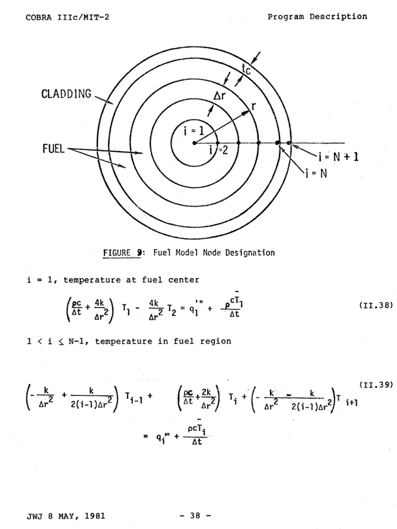
II.2.h Fuel Rod Heat Transport ... II.2.h.l The COBRA IIIc/MIT-1

II.2.h.2

Approach ...

The MATPRO Fuel Rod Model

II.2.h.2.1 Fuel and Cladding Material Properties II.2.h.2.2 Fuel-to-Clad Gap

Heat Transfer Coefficient ...

II.2.i BEEST Heat Transfer Model ....

II.2.j CHFR and CPR Correlations

II.2.j.l The W-3 and B&W2 CHFR

II.2.j II.2.j .2 Correlations ... CISE-4 CPR Correlation .. .3 Hench-Levy CHFR Correlation ... II.2.j.4 Biasi/Void-CHF Correlation ... II.3 Program Organization ... II.4 Subroutines ... 4.a 4.b 4.c 4.d 4.e 4.f 4.g 4.h 4.i 4.j 4.k Subroutine Subroutine Subroutine Subroutine Subroutine Subroutine Subroutine .Subroutine Subroutine Subroutine Subroutine AREA ... CHF ... ... DIFFER ... DIVERT ... FORCE ... HEAT ... ... MIX ... PROP ... SCHEME ... TEMP ... VOID ... 11.4.1 Other Subroutines ... 11.5 Functions ...

II.5.a Function HCOOL ... II.5.b Function S ...

11.6 Use of COBRA IIIc/MIT-2 ... 11.7 Nomenclature ... 37 37 39 39 40 40 42 42 45 46 46 49 51 51 51 51 52 52 52 53 56 56 56 58 58 58 58 58 59 60 iii II. II. II. II. II. II. II. II. II. IT. II.

III. INPUT DESCRIPTION ...

III.1 Introduction ... ...

111.2 Card Group 20 - The Recommended Input Method ... 111.3 Original Input Methods ... IV. SAMPLE PROBLEMS AND OUTPUT TABLES ...

IV.1 Lumped Channel Analysis

(IPILE = 0) Sample Problem...

IV.2 PWR Sample Problem

(IPILE = 1) ... _....

IV. 3 BWR Sample Problem

(IPILE = 2) ... ...

IV.4 Sample COBRA IIIc/MIT-2 Output

Tables ...

IV.5 Availability of the Actual Data Files and Calculation Results ... REFERENCES ... ... APPENDIX A: APPENDIX B: APPENDIX C: APPENDIX D: APPENDIX E: APPENDIX F: DERIVATION OF EQUATIONS

FOR FLUID TRANSPORT

MODEL ... 202

SUMMARY OF PRE-CHF CORRE-LATIONS USED IN OLD AND NEW

HEAT TRANSFER MODELS ... 209

SUMMARY OF CORRELATIONS PROVIDED FOR CALCULATION

OF DNBR, CHFR AND CPR .... 215 DERIVATION OF EQUATIONS

FOR THE OLD FUEL HEAT

TRANSFER MODEL ... 225 LISTING OF COBRA

IIIc/MIT-2 ... 229

SUGGESTIONS FOR POSSIBLE

IMPROVEMENTS TO COBRA IIIc/MIT-2 ... 408 iv PAGE 62 62 67 121 172 172 176 180 190 191 198

LIST OF FIGURES

FIGURE

NO. TITLE PAGE

1 METHOD OF SUBCHANNEL SELECTION ... 4

2 COBRA TRANSVERSE MOMENTUM CONTROL ... 15

VOLUME

3 TRANSVERSE MOMENTUM CONTROL, VOLUME .... 17 FOR WEISMAN APPROACH

4 TRANSVERSE MOMENTUM CONTROL VOLUME .... 18

FOR CHIU APPROACH

5 THE MATRIX [M] MODIFIED FOR FORCED .... 23 CROSS FLOW MIXING

6 THE 2 FACTOR IN THE BAROCZY TWO- .... 29

fo

PHASE FRICTION MULTIPLIER CORRELATION

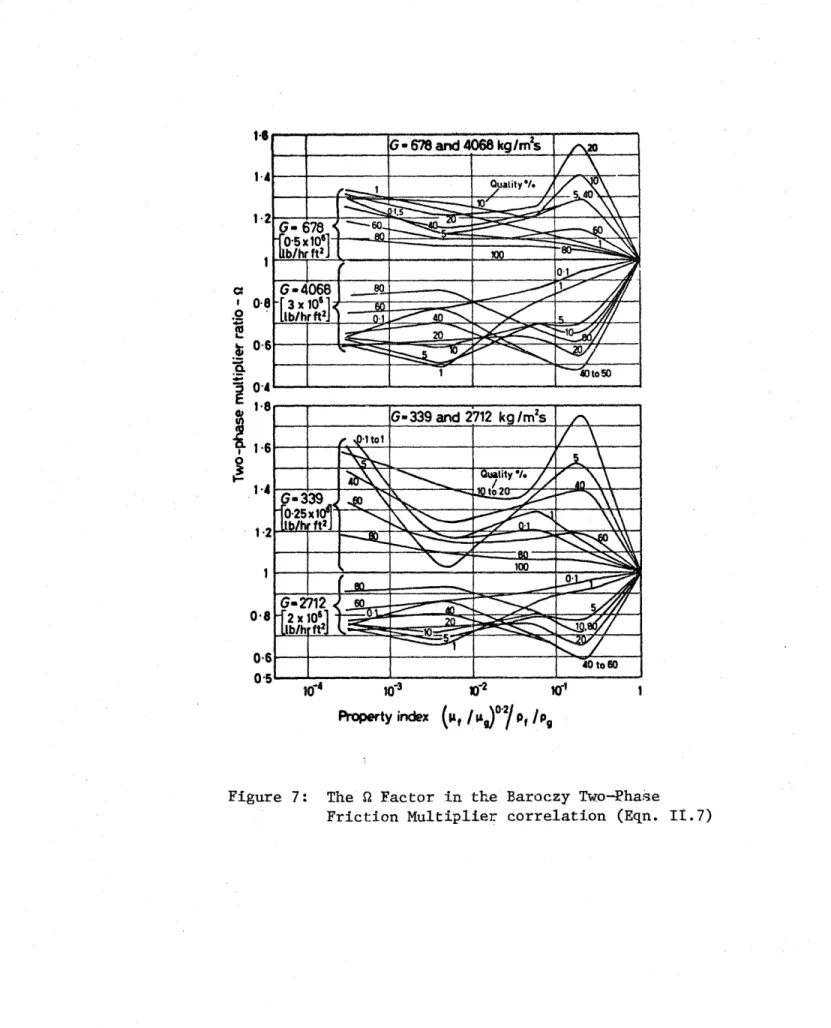
7 THE Q FACTOR IN THE BAROCZY TWO-PHASE .. 30

FRICTION MULTIPLIER CORRELATION

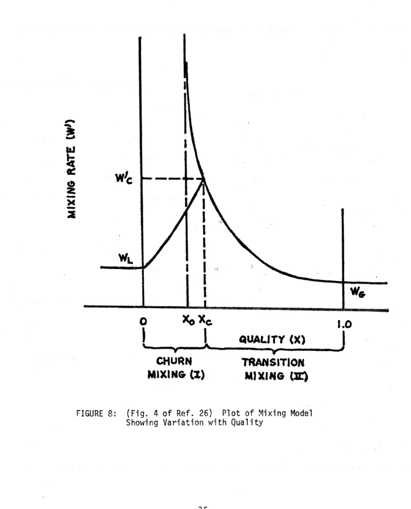
8 PLOT OF MIXING MODEL SHOWING VARIATION. 35 WITH QUALITY

9 FUEL MODEL NODE DESIGNATION ... 38

10 A TYPICAL BOILING CURVE OF BEEST ... 41 HEAT TRANSFER MODEL

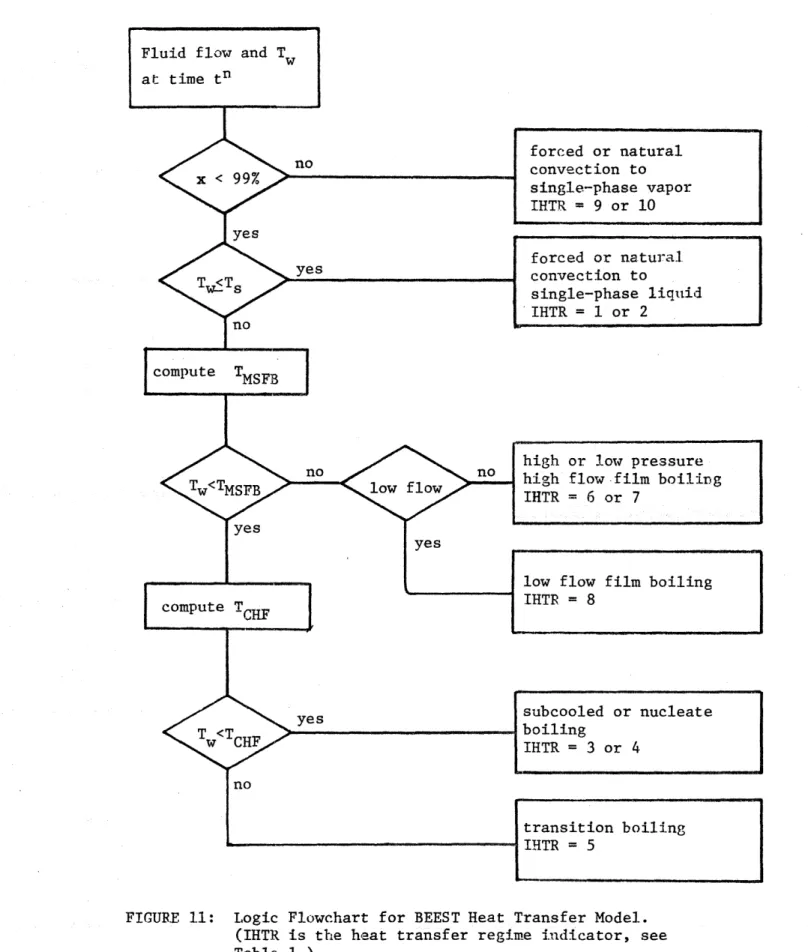
11 LOGIC FLOWCHART FOR BEEST HEAT ... 43 TRANSFER MODEL

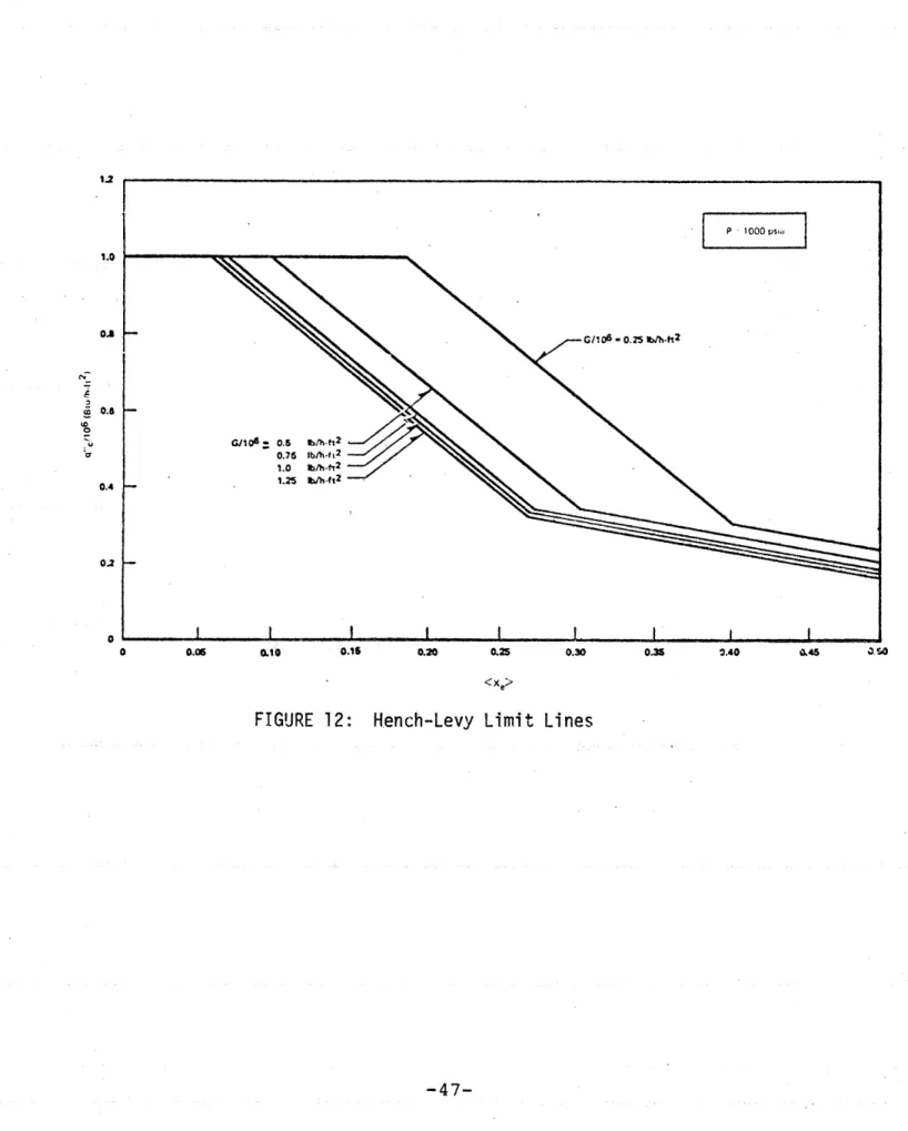
12 HENCH-LEVY LIMIT LINES ... 47

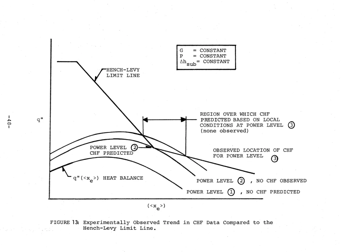
13 EXPERIMENTALLY OBSERVED TREND IN ... 48

CHF DATA COMPARED TO THE HENCH-LEVY LIMIT LINE

FIGURE

NO. TITLE PAGE

15 FLOW DIAGRAM OF LOGIC USED IN ... 54

SUBROUTINE "HEAT" WHEN A FUEL

ROD MODEL IS USED

16 FLOW CHART OF THE CALCULATION ... 57

PROCEDURE IN "SCHEME"

17 CHANNEL MAP AND REQUIRED CARDS ... 70

USING "IMAP" = 1

18 CHANNEL MAP AND REQUIRED CARDS ... 71

USING "IMAP" = 2

19 CARDS REQUIRED TO INPUT CHANNEL ... 73

MAP OF FIGURE 18 USING

"IMAP": = 3 INSTEAD OF 2

20 A) CHANNEL MAP FOR WHICH ONLY THE .... 74

"IMAP" = 3 OPTION WILL WORK

B) RESULTING INPUT DECK

21 CARDS OF TYPE 5-HF TO INPUT THE DATA . 76

OF TABLE 3 AND FIGURE 22

22 AXIAL HEAT FLUX PROFILE ... 77

23 CHANNEL MAP USING LUMPED CHANNEL ... 79

CONFIGURATION AND RELATIVE

ROD POWERS (RRP)

24 THE ARRANGEMENT OF CARDS 10-CD ... 85

THROUGH 12-CD TO INPUT CHANNEL DATA FOR THREE DIFFERENT

CHANNEL TYPES

25 CHANNEL MAP FROM WHICH THE COMBINA- .. 94

TIONS OF CHANNEL PAIRS AND BOUNDARY NUMBERS IN TABLE 4 WERE TAKEN

FIGURE

NO. TITLE PAGE

27 CHANNEL MAP FOR THE "IPILE" = 0 ... 173

SAMPLE PROBLEM

28 1/8 SECTION OF PWR CORE USED FOR ... 177

THE "IPILE" = 1 TEST CASE

29 CHANNEL AND ROD ARRANGEMENT USED ... 185

IN THE "IPILE" = 2 SAMPLE

PROBLEM

A-1 CONTROL VOLUME FOR THE CONTINUITY .... 202 EQUATION

A-2 CONTROL:VOLUME FOR THE ENERGY ... 203 EQUATION

A-3 CONTROL VOLUME FOR THE AXIAL ... 205 MOMENTUM EQUATION

A-4 CONTROL VOLUME FOR THE TRANSVERSE... 207 MOMENTUM EQUATION

D-1 ROD AND PLATE FUEL DIMENSION ... 228

EQUIVALENTS

LIST OF TABLES

TABLE

NO. TITLE PAGE

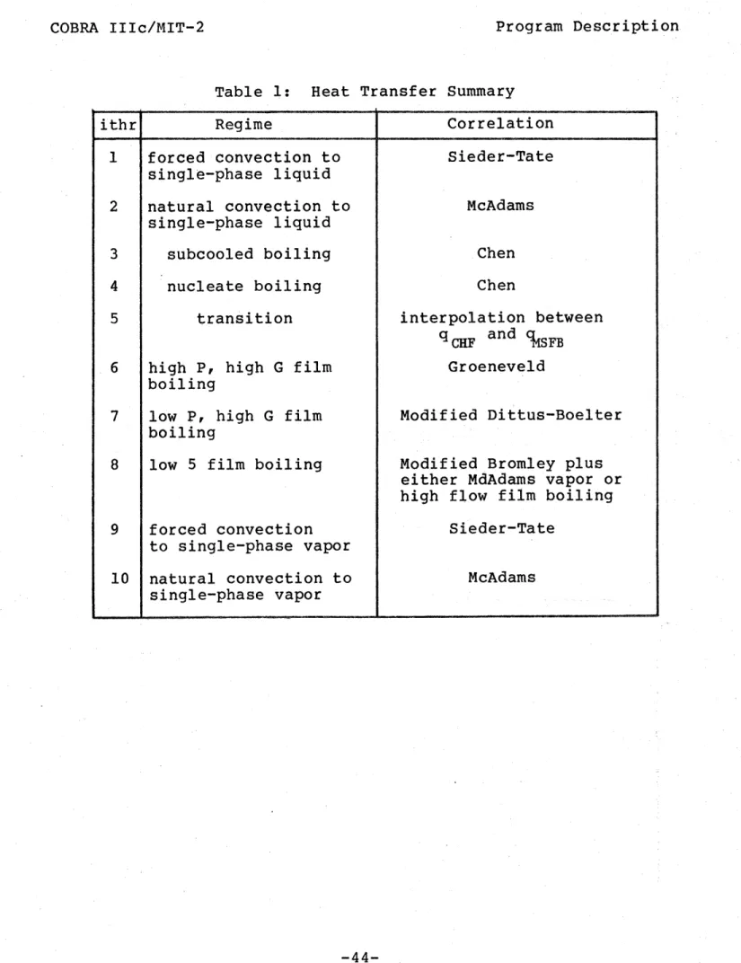
1 HEAT TRANSFER SUMMARY ... 44

2 AVAILABLE OPTIONS FOR CALCULATION ... 55

OF HEAT TRANSFER COEFFICIENT AND FUEL ROD TEMPERATURES

3 RELATIVE AXIAL HEAT FLUX DATA ... 77

4 THE CHANNEL PAIR - BOUNDARY NUMBER .. 94

COMBINATIONS RESULTING FROM THE CHANNEL MAP OF FIGURE 25

5 HEAT FLUX DISTRIBUTION FOR THE ... 174

"IPILE" = 0 TEST CASE

6 ROD INPUT DATA FOR THE "IPILE" = 0 .. 174

TEST CASE

7 THERMAL PROPERTIES FOR THE FUEL ... 175

MATERIAL IN THE "IPILE" = 0

TEST CASE

8 SPACER DATA FOR THE "IPILE" = 0 ... 175

TEST CASE

9 TRANSIENT FORCING FUNCTION DATA ... 175 POINTS FOR THE "IPILE" = 0

TEST CASE

10 THERMAL-HYDRAULIC MODEL OPTIONS .... 178 FOR THE "IPILE" = 0 TEST CASE

11 EXAMPLE PROBLEM INPUT DATA FOR ... 179 COBRA IIIc/MIT WITH "IPILE" = 0

12 AXIAL HEAT FLUX DISTRIBUTION FOR .... 180

THE "IPILE" = 1 TEST CASE

13 SPACER DATA FOR THE "IPILE" = 1 ... 181

TEST CASE

TABLE

NO. _TITLE

PAGE

14 _{THERMAL PROPERTIES FOR THE ... 181} FUEL MATERIAL IN THE "IPILE = 1

TEST CASE

15 _{THERMAL-HYDRAULIC MODEL OPTIONS ... 182} FOR THE "IPILE" = 1 TEST CASE

16 _{THE RADIAL POWER FACTORS FOR THE ... 182} RODS IN THE "IPILE" = 1 TEST CASE

17 _{SUBCHANNEL INPUT DATA FOR THE ... 183} "IPILE" = 1 TEST CASE

18 _{EXAMPLE PROBLEM INPUT DATA FOR ... 184} COBRA IIIc/MIT WITH "IPILE" = 1

19 _{AXIAL HEAT FLUX DISTRIBUTION FOR .... 186} THE "IPILE" = 2 TEST CASE

20 _{THE RADIAL POWER FACTORS FOR THE .... 186} RODS IN THE "IPILE" = 2

TEST CASE

21 _{SUBCHANNEL GEOMETRY DATA ... 187} 22 _{SPACER DATA FOR THE "IPILE" = 2 ... 187}

TEST CASE

23 _{THERMAL PROPERTIES FOR THE FUEL ... 187} MATERIAL IN THE "IPILE" = 2

TEST CASE

24 _{THERMAL-HYDRAULIC MODEL OPTIONS FOR .188} THE "IPILE" = 2 TEST CASE

25 _{EXAMPLE PROBLEM INPUT DATA FOR ... 189}

COBRA IIIc/MIT WITH "IPILE" = 2

26 _{COBRA IIIc/MIT-3 OUTPUT TABLE ... 192} SHOWING THE LENGTHS AND LOCATIONS

OF DATA ARRAYS STORED IN THE CON-SOLIDATED DATA ARRAY NAMED "DATA"

ix

. -.. :..

TABLE

NO. TITLE PAGE

27 COBRA IIIc/MIT-2 OUTPUT TABLE ... 193 OF CHANNEL EXIT SUMMARY RESULTS

28 COBRA IIIc/MIT-2 OUTPUT TABLE ... 193

GIVING BUNDLE AVERAGED RESULTS

29 COBRA IIIc/MIT-2 OUTPUT TABLE ... 194 GIVING INDIVIDUAL CHANNEL RESULTS

30 COBRA IIIc/MIT-2 OUTPUT TABLE ... 195

GIVING THE DIVERSION CROSSFLOWS BETWEEN ADJACENT CHANNELS

31 COBRA IIIc/MIT-2 OUTPUT TABLE GIVING . 196

FUEL ROD THERMAL RESULTS

32 COBRA IIIc/MIT-2 OUTPUT TABLE ... 197 SUMMARIZING THE CHF RESULTS

COBRA IIIc/MIT-2

PREFACE

This publication has been produced to reflect changes made to COBRA IIIc/MIT-1 since the manual was last updated (Ref. 1). The suffix "-1" is used to designate the original version of the code as reported in reference 1. The current version is denoted

by the suffix "-2". When the generic nature of both versions is

being referred to, the designation "COBRA IIIc/MIT" is used without any version number suffix. The major references in the

production of _{this updated manual were the COBRA IIIc/MIT-1}

manual, the original COBRA IIIc manual (BNWL-1695), and the various reports of modifications made over the years. The publications mentioned above are references 1 through 5 of the reference list. Many sections of this manual have been copied in full or in part from these sources, and the interested reader is refered to them for more detailed information concerning the origin, modifications, and testing of COBRA IIIc and COBRA IIIc/MIT. The reference from which the major portion of each section of was taken is indicated in the section heading.

The primary objective of this manual is to provide sufficient information to enable any student or engineer in the field of Thermal-Hydraulics to use COBRA IIIc/MIT-2 competently, and with

confidence. _{Recognizing that errors are always possible in a}

publication of this size, the entire text of this manual has been

stored on magnetic tape to facilitate correction. It is also

hoped that this manual will be updated to include any future modifications to COBRA IIIc/MIT.

A source listing of the code, the data files used for the

sample problems, and the printout results from the executions of the sample problems have also been stored on the same tape as the text of the manual. All corespondence concerning the contents of this tape, including corrections to the manual and requests for copies of the code should be addressed to:

Computer Code Librarian Nuclear Engineering Department Massachusetts Institute of Technology

Building NW-12 Room 230

138 Albany Street

Cambridge, Ma 02139

ATTN: Rachel Morton

JWJ 8 MAY 1981

Preface

COBRA IIIc/MIT-2

COBRA IIIc/MIT-2: A DIGITAL COMPUTER PROGRAM FOR STEADY

STATE AND TRANSIENT THERMAL-HYDRAULIC

ANALYSIS OF ROD BUNDLE NUCLEAR FUEL ELEMENTS

INTRODUCTION

This report presents the COBRA IIIc/MIT-2 computer program for performing both steady-state and transient subchannel analysis of

rod bundle nuclear fuel elements. COBRA IIIc/MIT-2 computes the flow and enthalpy in the subchannels of rod bundles during both boiling and nonboiling conditions by including the effects of crossflow mixing.

The subchannel analysis approach has become recognized as the standard method to analyze the steady-state thermal-hydraulic performance of nuclear fuel bundles. As a result, there has been considerable interest in using a similar analysis method for

transients. Much of the safety analysis of nuclear reactors is

related to the transient response of the reactor core and fuel following normal operating transients and potential accident

situations. The analysis of these transients with

one-dimensional analysis methods is not entirely complete. More sophisticated multi- dimensional analysis techniques provide a more detailed understanding of the thermal-hydraulic performance of nuclear fuel bundles during transients.

JWJ 8 MAY, 1981

Introduction

-COBRA IIIc/MIT-2

SUMMARY

The COBRA IIIc/MIT-2 computer program computes the flow and enthalpy in rod-bundle nuclear fuel element subchannels during both steady state and transient conditions. It uses a mathematical model which considers both turbulent and diversion crossflow mixing between adjacent subchannels. Each subchannel is assumed to contain one-dimensional, two-phase, separated, slip-flow. The two-phase flow structure is assumed to be fine enough to define the void fraction as a function of enthalpy, flow-rate, heat-flux, pressure, position and time. At the present time, steady-state two-phase flow correlations are assumed to apply to transients. The mathematical model neglects sonic velocity propagation; therefore, it is limited to transients where the transient times are greater than the time for a sonic wave to pass through the channel. The equations of the mathematical model are solved by using a semi-explicit finite difference scheme. This scheme also gives a boundary-value flow solution for both steady state and transients where the boundary conditions are the inlet enthalpy, inlet mass velocity, and exit pressure.

The features of COBRA IIIc/MIT-2 can be summarized as follows:

- It can consider transients of fast-to-intermediate speed. No sonic velocity propagation effects are considered.

- The numerical scheme performs a boundary value solution where the boundary conditions are the inlet flow, inlet crossflow, inlet enthalpy and exit pressure.

- The numerical solution has no stability limitation on space or time steps.

- The transverse momentum equation includes temporal and spatial acceleration of the diversion crossflow.

- Fuel pin model options allow calculation of fuel and cladding temperatures during transients by specifying power density.

- Forced flow mixing due to diverter vanes or wire wraps is included.

- The numerical procedures allow more complete analysis of bundles with partial flow blockages.

The inclusion of the temporal and spatial acceleration of the diversion crossflow provides a more complete physical model with only a small increase in the complexity of the numerical solution. The importance of these additional phenomena are governed by the parameters u*, C, and (s/l). These have only a small-to-moderate effect on subchannel flow solutions for most rod bundle analyses. The effect of these parameters should be evaluated and justified experimentally if they have important influence on the flow solutions.

JWJ 8 MAY, 1981

Summary

-COBRA IIIc/MIT-2

The use of fuel rod heat transfer models coupled with the subchannel analysis method provides a more complete way of performing transient thermal-hydraulic analysis of rod bundle

nuclear fuel elements. By selecting appropriate heat transfer

correlations the fuel temperature response to selected transients can now be analyzed in much greater detail.

While the use of an inlet flow boundary condition may be

entirely satisfactory for a wide range of problems, there are

many analyses where the pressure at each end of the bundle could be defined with greater ease. Cases involving transient flow reversal, coolant expulsion or countercurrent subchannel flow would require the use of other computer codes.

JWJ 8 MAY, 1981

Summary

-Mathematical Models

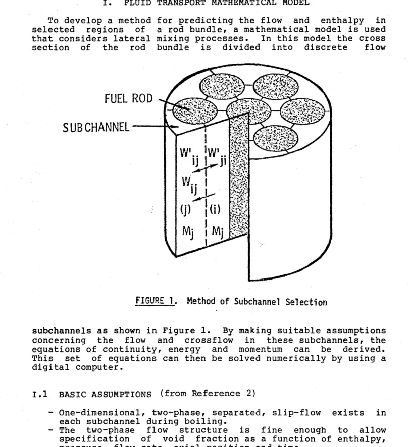
I. FLUID TRANSPORT MATHEMATICAL MODEL

To develop a method selected regions of that considers lateral

section of the rod

FUEL ROD

SUBCHANNEL

for predicting the flow and enthalpy in a rod bundle, a mathematical model is used mixing processes. In this model the cross

bundle is divided into discrete flow

FIGURE 1. Method of Subchannel Selection

subchannels as shown in Figure 1. By making suitable assumptions concerning the flow and crossflow in these subchannels, the equations of continuity, energy and momentum can be derived. This set of equations can then be solved numerically by using a digital computer.

I.1 BASIC ASSUMPTIONS (from Reference 2)

- One-dimensional, two-phase, separated, slip-flow exists in each subchannel during boiling.

- The two-phase flow structure is fine enough to allow specification of void fraction as a function of enthalpy, pressure, flow rate, axial position and time.

- A turbulent crossflow exists between adjacent subchannels that causes no net flow redistribution.

JWJ 8 MAY, 1981

COBRA IIIc/MIT-2

-Mathematical Models

- The turbulent crossflow may be superimposed upon a diversion

crossflow between subchannels that results from flow

redist-ribution. This may occur artificially from devices that

force diversion crossflow.

- Sonic velocity propagation effects are ignored.

- The diversion crossflow velocity is small compared to the

axial velocity within a subchannel.

The first four assumptions are those used in Meyer's (Ref. 8)

two-phase flow model which is assumed to apply to rod bundle

subchannels. The separated slip flow assumption is valid

provided that in the regions they occupy the separated phases have uniform properties and mass fluxs. This is not always the case, especially for annular flow (Ref. 9) where the liquid at the wall is at significantly lower velocity than the entrained

liquid drops. Although the separated flow assumption allows

considerable simplification of the momentum and energy equations, the limitations of the assumption should be realized by users of the COBRA IIIc/MIT programs. The last two assumptions greatly simplify the mathematical model and the numerical solution. Neglecting sonic velocity propagation is justified for moderate speed transients. Meyer justifies this assumption for transients with times that are longer than the sonic propagation time

through the channel.

The last assumption allows a transverse momentum equation to be derived by only preserving the vector direction between adjacent pairs of subchannels. In other words, the crossflow

loses its sense of direction when it enters a subchannel. This

assumption also allows the difference between transverse momentum

fluxes normal to the gap to be neglected. This assumption is

justified even for severe flow diversions.

1.2 EQUATIONS OF THE MATHEMATICAL MODEL (from Reference 2)

The equations of the mathematical model may be derived by using the previous assumptions and by applying the general equations of continuity, energy and momentum to a segment of an arbitrary subchannel, as shown in Appendix A. The derivations

are similar to those presented earlier (Ref. 5,6,7) and are

included here for completeness. For simplicity the equations are presented for an arbitrary Subchannel (i) which is connected to

another Subchannel (j). The equations are generalized later to

account for an arbitrary subchannel layout. The right side of the continuity equation

3p _Pi m._mi

A + = -ij (I.l)

JWJ 8 MAY, 1981 5

COBRA IIIc/MIT-2

gives the net rate of change of subchannel flow in terms of the diversion crossflow per unit length. By choice, the diversion crossflow is positive when flow is diverted out of Subchannel (i). The turbulent crossflow does not appear because it does not cause a net _{flow change. The time derivative of density gives} the component of flow change caused by the fluid expansion or contraction.

The right side of the energy equation Sah.

ah. q'. w'.. c. w..

1

_-t)

₎₃

U x mt m mi m -1 m i- mi (1.2)

contains three terms for thermal energy transport in a rod bundle fuel element. The first term is the power-to-flow ration of a subchannel and gives the rate of enthalpy change if no thermal mixing occurs. The _{second term accounts for the turbulent} enthalpy transport between all interconnected subchannels. The turbulent thermal mixing w' is analogous to eddy diffusion and is defined through empirical correlations.(Ref. 6) The third term accounts for the thermal conduction mixing. The fourth term accounts for thermal energy carried by the diversion crossflow. This is a convective term that requires a selection of the enthalpy h* to be carried by the diversion crossflow. The first term on the left side of Equation (1.2) gives the transient contribution to the spatial rate of enthalpy change. These are convective terms with a transport velocity u". Since u" represents the effective velocity for energy transport, the time duration of a transient is related to this velocity. Note that sonic velocity propagation effects are ignored by the absence of

a ap/at term.

The right side of the axial momentum equation

am. ap p _{2 v f k v'./A.} 1 1 1 1A 2u. +

=

-I-(u _{A. 1} - u ) w' + _A. i (2u. -_i u*)

w.

contains _{several terms that govern the axial pressure gradient} in a subchannel. _{Without the crossflow terms, these are the} frictional, spatial acceleration and elevation components of pressure gradient. _{The turbulent crossflow term tends to} equalize _{the velocities of adjacent subchannels. This is} analogous to turbulent stresses in turbulent flow. The factor fT is included to help account for the imperfect analogy between the turbulent transport of enthalpy and momentum. The diversion

JWJ 8 MAY, 1981

Mathematical Models

-Mathematical Models

COBRA IIIc/MIT-2

crossflow term accounts for the momentum changes due to changes in subchannel velocity. The first two terms on the left side of Equation (1.3) are the transient components of the axial pressure gradient.

Appendix A presents a derivation of a more complete transverse momentum equation that more properly accounts for the crossflow

momentum coupling. For two adjacent subchannels this equation

can be written as

w. u*..w..

aw

.c

w

"

;t +x 1-C w =J (P i- pj) (1.4)

The first two terms represent the temporal and spatial

acceleration (1) of the crossflow. The remaining two terms are

the friction and pressure terms used in an earlier transverse momentum equation. (Ref. 5,6,7) The new parameter (s/l) represents the importance of friction and pressure terms versus the inertial terms. These inertial terms also represent the transport of the

crossflow at axial velocity u*- . These terms cause the

crossflows to persist as they move town the channel. This is the "axial inertia" effect often included in crossflow resistence

correlations. (Ref. 6,10) The friction term is a linearized

representation of fluid friction; however, COBRA IIIc/MIT

presently considers C** to be a nonlinear function that depends on the absolute value o the diversion crossflow.

The primary assumption used to derive Equation (1.4) is that the crossflow through a rod gap loses its sense of direction upon enering or leaving a subchannel and that the difference in lateral momentum flux is small. The direction of the crossflow

is only considered between the two interconnecting subchannels of

interest. This assmption is valid if the crossflow velocities

are small compared to the axial velocities. This is usually the case for most computations in nuclear rod bundles.

An equation of state of the form

Pi = p(h p*,mi x,t) _(1.5)

is used to define the two-phase fluid density. This equation can

be obtained by using an appropriate correlation for void

fraction. Selection of the appropriate correlation for the case

being analyzed is left to the user. Several void fraction

correlations are provided as options in the code.

(1) A term analogous to a(pv2 )/ay has been ignored in relation to a term analogous to3(Puv)/ax by the assumption of small crossflow

velocity. This can be justified by an order of magnitude

analysis

-Mathematical Models

For a large rod bundle the previous equations become unwieldy; therefore, a more compact form is very desirable. Reference 7 presents a vector form of the equations by using a matrix transformation IS] and its transpose [S]T. Using the IS]

transformation the previous equations may be written as follows: Continuity

S

-] {w}

(1.6)

_}

. - 2 u + = {a'} + [A]-1 2u] [S]T - [sIT[u* {w} (1.8)

Transverse Momentum

t + u (){cw} + ()[S]{p} (1.9)

where

{a'} = )( + x (v/A(I.10)

- fT[A]-1 [S]T [Au]{w'}

The elements of the matrix IS] are defined through two column vectors i(k) and j(k) where, for each pair of connected subchannels (i,j), a unique connection (or gap) number k is assigned. The connection numbers are assigned in ascending order

by considering Subchannel (i) and then assigning a unique connection number for each successively connected Subchannel (j) where j is greater than i. By using this identification

procedure the crossflows can be written as wk where k implies the subchannel pair i(k), j(k). For w > 0 the crossflow is chosen to be from Subchannel (i) to Subchannel (j) where i is less than

JWJ 8 MAY, 1981 COBRA IIIc/MIT-2

-Mathematical Models

j. The elements of the matrix IS] are defined as: S ki=0;

except, Ski=1

, if i=i(k); and Ski=-l, if i=j(k). 1.3 METHOD OF SOLUTION

The previous equations are solved as a boundary-value problem by using a semiexplicit finite difference scheme. The boundary conditions selected for the problem are the inlet enthalpy, inlet flow, inlet crossflow, and exit pressure. Initial conditions for enthalpy, flow, and crossflow distribution are established from

an initial steady-state calculation. _{No inlet condition for}

pressure is required as it is determined from the other boundary conditions and resulting solution. Solving the problem this way is an improvement over the initial-value solutions that are used in many subchannel analysis computer programs. While the use of the initial value solution can be justified as an approximation to the boundary-value solution if the crossflow resistance is small, it restricts the solutions to a limited class of problems.

Equations (I.6) through (1.9) are solved by using a finite

difference procedure. _{Finite difference node interfaces are}

numbered starting at the inlet end of each node. The location at the end of the last node is N+l where N is the number of nodes. Enthalpy, flow, pressure and crossflow are defined at the node interfaces. Boundary conditions for enthalpy, flow and crossflow are set at the channel inlet (J=l) and the exit pressure boundary

condition set at the channel outlet (J=N+1). _{The distance x=O}

corresponds to J=l and x=L corresponds to J=N+1. The finite

difference scheme is written for an interval J-1 to J

corresponding to xj_-1 and x. respectively.

The finite difference analogs to Equations (1.6) through (1.9) are: (1)

Continuity

i _J

1+

f

JWJ 8 MAY, 1981

(1) _{The overscore bar (i) indicates previous time.}

COBRA IIIc/MIT-2

-COBRA IIIc/MIT-2 Energy

I

h

r--

.[s)T

[h

mi

at

a

At

3

aJ+[Aj] 1 2u S] -S] [u* .JiWi

Transverse Momentum (1.13) r k *W. - U At

J

.w

Equations (I.11), (1.13) and (1.14) can be combined to eliminate

{P ) and {m)}. Let {a'j in equation (1.13) be written as

j-1 3 i

a' j = {Kmj2- fj} (I.15)

where Kjrepresents coefficient of the flow-squared terms and {fg) are the remaining terms of {a'j ). Now let

mi

=

=

mj-1

(1.17) where Am = -[S]Tfwj Ax - Aj (pj - p )Ax/At

Squaring mj gives

tj 2j

j-1

2 _{+ (2mj-1+Am) +Am (I.18)}

JWJ 8 MAY, 1981

(I.12)

- 10

-Mathematical Models

COBRA IIIc/MIT-2

Normally Am2 would be discarded as being small, however, for flow

blockage analysis Am can be as large as m. It can be retained by using the following form for Equation (I.18)

m2 2 + (2 + Am) A(I.18a)

and upon substituting Equation (1.16) it becomes

{2J; 2'. + (m _{I +}

_)}

j J rI Y M (I.19)

The value of m_i on the right side is unknown but it can be

initially estimated and updated through iteration. By using Equations (1.13), (1.15), and (1.19) the pressure at J-1 can be written as {-1 {p - F}Ax - [Rj

Wj}

JR

-

_{] [s}

[Es)T

(m,

{K

m2

{}

{

(

The pressure difference between subchannels can now be written as

IS] [S] - [S) {Fj} Ax - [S] [R1 j Ax (1.23)

Substituting this result into Equation (1.14) to eliminate

[S]{Pj-1 ) gives a set of simultaneous equations of the form

l {w4d=fbMj (1.24)

JWJ 8 MAY, 1981 - 11

Mathematical Models

where

[MJ

I1

]

+

(})

[cx

+([R]

_x

₍₂₅₎

and

(u*w)J +

()

[

The first three items on the right side of Equation (1.25) are

diagonal matrices. _{The first two of these come from the added}

temporal and spatial acceleration terms in the transverse

momentum equation. They are also very important as they provide additional numerical stability. Reducing Ax and At adds more diagonal dominance and thus more stability to the numerical solution. However, beyond a certain value reducing the mesh size may begin to increase the number of iterations required to

achieve convergence due to the marching solution proceedure. As in earlier difference schemes (Ref. 5,6,7) the last term on the right side of Equation (1.25) includes a matrix which is singular for any rod bundle problem with a lateral transverse flow loop. The additional terms in Equation (I.25) remove the singularity

and thus allow a unique solution for the crossflow. Two

additional terms are included in Equation (1.21), one is a term

to account for the axial friction pressure loss at xj. This is a

very important term for flow blockage analysis because it allows the calculation to look downstream and account for a sudden large change in the friction pressure gradient. The other term Ax/At

in Equation (1.21) accounts for rapid changes in the flow m..

The matrix [M] _{controls the distribution of crossflow;}

however, the vector _{(b) contains the crossflow forcing terms.}

The first two terms on the right side of Equation (1.26) try to maintain the crossflow that existed at previous time or space.

If other forces did not exist, crossflow would tend to persist.

The third _{term is the pressure difference affecting the}

crossflow. _{This is also the term that feeds downstream}

information _{into the crossflow solution. The fourth term}

provides the basic driving force for crossflow. If the pressure

gradients due to _{friction, acceleration and gravity are}

unbalanced, crossflows occur in an attempt to equalize them.

1.4 DISCUSSION OF PARAMETERS _{(from Reference 2)}

Solutions to the previous set of equations require a certain

amount of empirical information. _{Because of the incomplete}

knowledge of steady state and transient two-phase flow in bundles

some of this information must be supplied by assumption. For

JWJ 8 MAY, 1981 COBRA IIIc/MIT-2

-Mathematical Models

COBRA IIIc/MIT-2

example, h* and u* are commonly assumed to be their respective values from the donor subchannels. Other selections of u* and h*

may be made(Ref. 11) to account for the nonuniform enthalpy

distribution in a subchannel. This usually requires information

about the liquid-and-vapor-phase distribution. The factor fT

used to account for the _{imperfect analogy between eddy}

diffusivity of heat and momentum is also unknown but its effect

is weak. For many problems fT can be safely set equal to

zero.(Ref. 5) The correlations required for calculating the pressure gradient are of major importance. This includes the correlations for friction factor, subcooled void fraction, bulk void fraction and two-phase friction multiplier. Fortunately, correlations of these effects developed for simple channels (Ref. 12-15) may be applied to rod bundle subchannels for steady

state with reasonably good results (Ref. 16-18). Since their

accuracy is questionable for high speed.transients, additional experimental work is needed in this area. Turbulent mixing must also be specified from empirical correlations or data. At the present time a definitive correlation for mixing does not exist for all bundle geometries and all flow conditions. Some progress has been made to describe mixing for single (Ref. 19,20,21) and two-phase (Ref. 11,17,18) flow; however, very little is known about two-phase mixing processes during transients.

The transverse momentum equation and fuel heat transfer model add still more parameters to the subchannel analysis method.

These parameters and their effect on typical rod bundle

calculations are discussed in the succeeding sections.

1.5 TRANSVERSE MOMENTUM EQUATION PARAMETERS (from Reference 2) The transverse momentum equation introduces the parameter

(s/l) and also underscores importance of the terms u* and C.

Some insight concerning the importance of these parameters can be found by inspecting the finite difference form of the combined transverse momentum equation, Equation (1.24). For discussion

purposes, consider the matrix [M] for two interconnected

subchannels of equal area. (1) The matrix has only one element given by

m + + C +- Ax (1.27)

-- m=-1-- _-

---(1) _{A similar equation for unequal areas shows that a sign change}

leading to instabilities can occur depending upon the subchannel

velocities and flow areas. This is a source of computation

failure of COBRA IIIc/MIT when subchannel areas are highly nonuniform.

-Mathematical Models

where u* is the average of the two subchannel velocities. The

relative importance of the terms can be controlled by arbitrarily selecting Ax. The second and fourth terms can be made comparable

magnitude by selecting s/1 = 1/2 and Ax2 _{=A which usually}

requires Ax < 0.5 inch for typical nuclear reactor rod bundle

problems. _{A larger value of AX is normally used as it reduces}

computation time for long bundles. In those cases the last term is the largest one. The smallest term is usually the transverse

friction term, C. It contains the friction coefficient K which

could be expected to be on the order of unity or less. This

friction coefficient does not include an "axial inertia" term contained in some previous crossflow resistance correlations. (Ref. 19,10) It is improper to use those correlations here because the "axial inertia" effect is contained in the transverse momentum term u*/Ax. This can be seen by writing the pressure

difference Pi-P. = u*dw/dx. If dw is approximated by w and if dx

is approximate by an appropriate length, then, P.-P. (u*/v)v2

and the resistance coefficient due to axiali Inertia is

proportional to u*/v. _{This ratio is large for small crossflow}

velocity. The same result is reported in a combined momentum and friction crossflow correlation by Khan (Ref. 10) at large values

of u*/v. _{At small values of u*/v Khan's correlation reduces to}

Ki z 0.25 which would presumably be an estimate of the friction

coefficient for pure crossflow. This discussion points out the

usual dominance of u*/Ax over (s/l)C. The values of C are

therefore relatively _{unimportant for most problems. This}

conclusion may not be true, however, for very closely spaced rod bundles since C is believed to be nearly inversely proportional to the square of the gap spacing.

The (s/l) parameter appears in all but the transverse momentum terms; therefore, as long as u*/Ax and l/At are small components

of [MI, (s/l) is a weak parameter. Since this is usually the

case for the value of Ax used in rod bundle analysis (s/l) need

not be specified to high accuracy. For core-wide analysis of pressurized water reactors this conclusion may not be valid because Ax2 may be small compared to A.

The velocity u* appears in the transverse and axial momentum

terms. Since these are usually the the largest components of

[M], u* could have a stronger effect on crossflow solutions than

the previously discussed parameters. The choice of u* must

presently be made by assumption because of insuficient data to define it accurately. Fortunately, a variety of assumptions can be made that give comparable values of u*. This is because most bundles have rather uniform subchannel velocity distributions. The most serious errors in u* could ocur where large subchannel velocity differences occur. In those cases the effect of the u* assumption should be checked.

The previous comments concerning the usually small magnitude of u*/Ax and C does not mean that they can be dropped from the

JWJ 8 MAY, 1981 - 14

COBRA IIIc/MIT-2

calculations. They play a vital role in the numerical stability.

As discussed previously, part of the matrix tM] is a singular

matrix for any problem where one or more transverse flow loops exist such as around a fuel rod. In those cases the crossflow

around the loop is not unique. Including u*Ax and C removes the

singularity by imposing the friction and momentum constraint that the sum of the pressure drop around a transverse loop is equal to

zero. Mathematically these terms add diagonal dominance to [M],

thus, improve the condition of [M]. The diagonal dominance can

be improved by decreasing Ax.

1.6 THREE APPROACHES FOR COBRA IIIC/MIT-2 (from Reference 3)

TRANSVERSE MOMENTUM MODELING

Weisman (Ref. 22) has suggested that the transverse momentum paramaters used in COBRA IIIc/MIT, s/l and K_i , should be modified when the code is used for analysis cases involving interconnected regions of different size. This suggestion has also been made by Chiu (Ref. 23). COBRA IIIc/MIT-2 provides the option of using the Weisman and Chiu approaches in addition to the old COBRA approach for transverse momentum modeling.

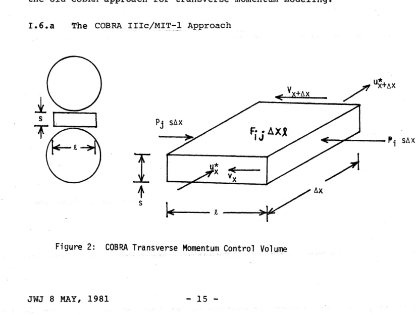
I.6.a The COBRA IIIc/MIT-1 Approach

V X AX

P. SAX

vx

Figure 2: _{COBRA Transverse Momentum Control Volume}

JWJ 8 MAY, 1981 - 15

Mathematical Models

The old COBRA approach (Ref. 2) is based on conserving transverse momentum in a control volume for the gap between two subchannels as shown in Figure 2. By conservation of momentum, the following equation is obtained:

a

at [Wij] + Pxi . Fij

where

2Sij) P * (I.29)

and

Wij = diversion crossflow between subchannels i and j (lbm/hr ft)

u* = effective velocity carried by diversion crossflow (ft/sec)

x= axial distance (ft)

s = width of gap between rods (ft)

1 = effective length of connection between subchannels (ft)

P. = pressure in channel i (lbf/ft2) 1

P = pressure in channel j (Ibf/ft 2 )

K = crossflow coefficient (dimensionless)

S.. = total gap width connecting channels i and

j

sulchannel analysis) [ft]

p* = density of the diversion crossflow (ibm/ft3 )

I.6.b The Weisman Approach (from Reference 3)

The Weisman approach (Ref. 22) casts the transverse momentum

equation in a more general form, allowing interconnection of different-sized channels.

a

xat

Mathematical Models COBRA IIIc/MIT-2 where S.

-j

=

j

gaps through which flow between channels i

(Nr) = number of rods between centers of channels i and j.

For subchannel or bundle-to-bundle analysis, N = N for all

flow region interconnections. Thus, the Weisman ipproich reduces to the old COBRA approach for such analyses. Figure 3 shows two interconnected regions of different size, a situation where the Weisman anproach applies.

Region i

p---Reqion

Figure 3: Transverse Momentum Control Volume for Weisman Approach

JWJ 8 MAY, 1981 where

(1.32) (1.33)

-COBRA IIIc/MIT-2

I.6.c _{The Chiu Approach (from Reference 3)}

The Chiu approach (Ref. 23) differs from the Weisman approach in the _{control volume used. Chiu uses the interaction of the} adjacent rows of subchannels of two regions to represent the interaction between two regions, as shown in Figure 4. This

Region i

Figure 4:

S

J

Transverse Momentum Control Volume for Chiu Approach

approach uses the following transverse momentum equation.

D(u*W ) S.. (P - P.) t x (NP) ij - F. where KIW ijlWij S.. S ijT 2 2 (S._.) p* (I.34) (I.35) and (P P.) (Np) i = -P3 (Pi P-) JWJ 8 MAY, 1981 (I.36) Mathematical Models - 18

-Mathematical Models

where

(Np)i = the pressure transport coefficient for subchannels

adjacent to the boundary between subchannels i and j.

Pi = pressure in interacting subchannel(s) of channel i

adjacent to gap interconnection ij (Ibf/ft2).

P = pressure in interacting subchannel(s) of channel j adja ent to gap interconnection if (lbf/ft2).

During the development of the single-pass method (Ref. 24), use of the pressure transport coefficient was found to have

little effect upon COBRA IIIc/MIT enthalpy predictions,

especially in comparision to changes resulting from use of an

enthalpy transport coefficient in COBRA's energy equation. Both

pressure and enthalpy transport coefficients were found to be

unnecessary for single-pass MDNBR analysis under conditions

without strong crossflow.

I.6.d The Combined COBRA IIIc/MIT-2 Approach (new)

By noting the similarities between the three approaches, a combined set of equations was derived.

j

a(u*wL)

(1.37)

[Wj] + I (fs) a - P (1.37)

E ij S(P - ) ij

L2(Sj) p, " s)k ij (I.38)

By proper selection of the constants, (f ),j and (f ) any

of the three models can be used, s 2 sk ij

For the Weisman approach,

N

(fs)ij

()i

(I.39a)

(f sk)j (N )ij _(I.39b)

JWJ 8 MAY, 1981 - 19

Mathematical Models

For the Chiu approach,

(N )

(ff ) (Ni : (I.40a)

(fa ij (N)ij

(I.40b)

When a user does not select the new transverse momentum

option, the fs₈ and factors are set to unity and the old COBRA approach will be used.

1.7 FORCED CROSS FLOW MIXING (from Reference 2)

The previous finite difference scheme allows forced diversion cross- flows to be specified. This feature allows the effects of forced flow diverter vanes and forced crossflow mixing from wire wrapped bundles to be considered.

COBRA IIIc/MIT includes a forced crossflow mixing model which was originally developed for the COBRA II program(Ref. 6) but not published. Initial calculations with COBRA II were not entirely satisfactory because the numerical solution was not a boundary-value flow solution. The absence of the boundary-value solution allowed crossflows to increase fictitiously around the periphery of a bundle as the bundle size was increased. The method of solution did not allow the forced flow diversions to

redistribute flow axialy. The boundary-value solution used in COBRA IIIc/MIT allows these calculations to be included on a more realistic basis. The following model is the one contained in COBRA IIIc/MIT-2.

P/2

Consider the wire wrap as it passes from one subchannel to another as shown in the sketch. Where the wrap crosses the minimum part of the gap the slope of the wrap imposes a

transverse velocity given by

D+t

uij

=

JWJ 8 MAY, 1981 - 20

Mathematical Models

If this is multiplied by the fluid density and gap spacing the crossflow per unit length becomes

w = PSU = T _(1.42)

ij Pis juij *1

This equation applied at the gap only. When the wrap is

sufficiently far away from the gap it probably has little or no

effect on forcing flow through the gap in question. It is now

postulated that there is some function f(x/P) that periodically defines the importance of Equation (1.42) for defining the forced crossflow through a chosen gap. This function may look something

like the one in the following sketch.

1

f(/P)

0,

x/P

The rise in the function represents the approach of the wire

toward the gap. The function peaks at 1.0 according to Equation

(1.42) and then decays as the wrap moves away from the gap. The

area under the curve represents the fraction of flow diverted through the gap as compared to the total possible flow that could

be carried by a wrap over an entire pitch length. Since the

shape of this function is not known, the pulse is assumed to be a rectangular pulse with width a. The forcing function is then f(x/p) = 0, except for

f(x/p) =1 ; (x /P -6/2) < x.< (xc P + 6/2) (1.43)

For computations in COBRA IIIc/MIT it is presently assumed that the flow carried through a gap by a wrap occurs over one node length, Ax. The total flow diverted is; therefore,

wDividing gives the crossflow 6P this by Ax (1.4)

Dividing this by Ax gives the crossflow per unit length over one

JWJ 8 MAY, 1981 - 21

Mathematical Models

node length

Wforced =x Ai ; x-Ax .45)

This equation shows that a fraction of the subchannel flow m is

diverted from one subchannel to another when a wrap crosses a gap at axial position x when x-Ax < x < x.

C -- C

The calculations also correct the subchannel flow area and wetted perimeter for the number of wraps in a subchannel at each axial position.

The specified value of forced crossflow is included by simply modifying Equation (1.24). Suppose the crossflow in gap k is to

be specified. First the right side (b) must be modified. For

each k = £

bk

bkmod =forted

and for k = 1

mod forced (1.47)

The matrix [M] is modified by setting row k and column k equal to

zero except MU = 1. As an example if P = 3 the matrix

modification would be that shown in Figure 5. The same procedure applies if more than one crossflow is being forced.

Forced crossflow mixing due to diverter vanes is considered in

much the same way. _{When subchannel grid spacer losses are}

specified for input to COBRA IIIc/MIT, a flow diversion fraction

is specified where the fraction is defined by the ratio w..Ax/mi.

if wj > 0 and wj Ax/m if w < 0.

The previous method of considering forced crossflow should be considered tentative until experimental data are available to check the validity.

1.8 COMPUTATION PROCEDURE

Steady-state computations are performed first to obtain

initial conditions for the transient. Since the previously

presented finite difference equations are stable for large time steps, those same equations are used for the steady state calculations by setting At equal to some arbitrarily large value.

JWJ 8 MAY, 1981 - 22

Mathematical Models M l M12 0 M1 4 Mn W _{bl-M 3 w3}

forced

FIGURE 5: The Matrix [M] Modified for Forced Cross Flow Mixing with k = 3

An iteration is performed until convergence of the flow solution

is obtained. _{Convergence is achieved when the change in any}

subchannel flow is less than a user selected fraction of the flow from the previous iteration.

For each iteration the computation sweeps from the inlet to

the exit of the channel. _{With inlet boundary information on}

flow, crossflow and enthalpy given, the enthalpy can be advanced one space step by using Equation (I.11). For the first iteration the flow {m.} is set equal to (mi- 1 } otherwise the value from the

previous iteration is used. The crossflow solution is performed by solving Equation (1.24) with the previous iterate value of the

subchannel difference _{[S]{p _ After the crossflow {w I is}

calculated, _{{mj ) is calculAted using equation (I.11), and SI]{p}}

is calculated from Equation (1.23) and saved for use during the

next iteration. Note that [S]{p I is downstream of [S]{p 1 );

therefore, iteration allows the downstream pressure diffe nces to be felt at upstream locations. At the end of the channel the boundary condition is that the pressure difference between the

channels is zero (i.e. [S]{p) = 0). _{In this way a boundary}

value solution is obtained. Only a few iterations are sufficient for convergence because the pressure difference IS]{p) only propagates a few nodes for most problems.

The above equations do not require actual pressure since pressure difference is only used in the combined momentum

JWJ 8 MAY, 1981 - 23

Mathematical Models

equation. The calculation of pressure is, therefore, only a back calculation. It is calculated from Equation (1.13) in a forward

direction. _{When the exit is reached the pressures are set equal}

to the exit pressure.

Transient calculations are performed in the same way but for a

selected time step At. Boundary conditions and other forcing

functions are set to their desired values at the new time; then, the calculation sweeps through the channel for the number of iterations required to achieve convergence on the crossflow. The converged solution is used for the new initial condition and the procedure continues for all time steps.

JWJ 8 MAY, 1981 - 24

Program Description II. COMPUTER PROGRAM DESCRIPTION

COBRA IIIc/MIT -2 should be thought of as an automated solution

to _{the basic set of differential equations of the mathematical}

model. To actually perform this solution, the user must provide input. This input not only includes the geometric parameters and operating conditions, but also the various required empirical or semiempirical correlations. Any set of correlations can give a solution, but some correlations will give better solutions. At the present time, guidelines have not been established for complete selection of these correlations; therefore, the COBRA

IIIc/MIT-2

program does not contain a pre-selected set of input

correlations. _{Several correlations are provided for examples,}

but the final selection must be made by the user. Considerable

work is required to define correlations and flow modeling applicable to rod bundle transients. The applicability of the two-phase flow model should always be evaluated by the user. Users should also justify use of COBRA for any analysis outside

the range of experimental verification. _{Experiments may be}

required in some cases to verify application of COBRA.

The following sections present the general features of the COBRA IIIc/MIT-2 program, an illustrated description of the

pro-gram organization and a description of the propro-gram's subroutines.

II.1 GENERAL FEATURES _{(from Reference 2)}

The significant features of COBRA IIIc/MIT include the following: - It considers both steady-state and transient flow in rod

bundle fuel elements.

- It performs a boundary-value flow solution that permits the

influence _{of downstream flow disturbances to be felt}

upstream.

- _{It can consider both single- and two-phase flow.}

- _{It considers the effects of turbulent and thermal conduction}

mixing throughout the bundle by using empirically determined mixing coefficients.

- It includes mixing which results from the convective

transport of enthalpy by diversion crossflow.

- It includes the momentum transport between adjacent

subchannels which results from both turbulent and diversion crossflow.

- _{It includes the effect of temporal and spatial acceleration}

in the transverse momentum equation.

- _{It includes the effect of transverse resistance to diversion}

crossflow.

- _{It can consider an arbitrary layout of fuel rods and flow}

subchannels for analysis of most any rod bundle

JWJ 8 MAY, 1981 - 25