HAL Id: insu-02987271
https://hal-insu.archives-ouvertes.fr/insu-02987271
Submitted on 3 Nov 2020
HAL is a multi-disciplinary open access
archive for the deposit and dissemination of
sci-entific research documents, whether they are
pub-lished or not. The documents may come from
teaching and research institutions in France or
abroad, or from public or private research centers.
L’archive ouverte pluridisciplinaire HAL, est
destinée au dépôt et à la diffusion de documents
scientifiques de niveau recherche, publiés ou non,
émanant des établissements d’enseignement et de
recherche français ou étrangers, des laboratoires
publics ou privés.
Distributed under a Creative Commons Attribution - NoDerivatives| 4.0 International
License
Regional modelling of tracer transport by tropical
convection – Part 1: Sensitivity to convection
parameterization
Joaquim Arteta, V Marécal, E.D. Rivière
To cite this version:
Joaquim Arteta, V Marécal, E.D. Rivière. Regional modelling of tracer transport by tropical
con-vection – Part 1: Sensitivity to concon-vection parameterization. Atmospheric Chemistry and Physics,
European Geosciences Union, 2009, 9 (18), pp.7081-7100. �10.5194/acp-9-7081-2009�. �insu-02987271�
www.atmos-chem-phys.net/9/7081/2009/ © Author(s) 2009. This work is distributed under the Creative Commons Attribution 3.0 License.
Chemistry
and Physics
Regional modelling of tracer transport by tropical convection –
Part 1: Sensitivity to convection parameterization
J. Arteta1, V. Mar´ecal1, and E. D. Rivi`ere2
1Laboratoire de Physique et Chimie de l’Environnement et de l’Espace, CNRS and Universit´e d’Orl´eans, 3A avenue de la
recherche scientifique, 45071 Orl´eans cedex 2, France
2Groupe de Spectroscopie Mol´eculaire et Atmosph´erique, Universit´e de Reims Champagne-Ardenne and CNRS, Facult´e des
sciences, Moulin de la Housse, B.P. 1039, 51687 Reims Cedex, France
Received: 29 December 2008 – Published in Atmos. Chem. Phys. Discuss.: 4 March 2009 Revised: 21 July 2009 – Accepted: 19 August 2009 – Published: 24 September 2009
Abstract. The general objective of this series of papers is
to evaluate long duration limited area simulations with ide-alised tracers as a tool to assess tracer transport in chemistry-transport models (CTMs). In this first paper, we analyse the results of six simulations using different convection clo-sures and parameterizations. The simulations are using the Grell and D´ev´enyi (2002) mass-flux framework for the con-vection parameterization with different closures (Grell = GR, Arakawa-Shubert = AS, Kain-Fritch = KF, Low omega = LO, Moisture convergence = MC) and an ensemble parameteriza-tion (EN) based on the other five closures. The simulaparameteriza-tions are run for one month during the SCOUT-O3 field campaign lead from Darwin (Australia). They have a 60 km horizontal resolution and a fine vertical resolution in the upper tropo-sphere/lower stratosphere. Meteorological results are com-pared with satellite products, radiosoundings and SCOUT-O3 aircraft campaign data. They show that the model is gen-erally in good agreement with the measurements with less variability in the model. Except for the precipitation field, the differences between the six simulations are small on average with respect to the differences with the meteorological obser-vations. The comparison with TRMM rainrates shows that the six parameterizations or closures have similar behaviour concerning convection triggering times and locations. How-ever, the 6 simulations provide two different behaviours for rainfall values, with the EN, AS and KF parameterizations (Group 1) modelling better rain fields than LO, MC and GR (Group 2). The vertical distribution of tropospheric tracers is very different for the two groups showing significantly more transport into the TTL for Group 1 related to the larger
av-Correspondence to: J. Arteta
erage values of the upward velocities. Nevertheless the low values for the Group 1 fluxes at and above the cold point level indicate that the model does not simulate significant over-shooting. For stratospheric tracers, the differences between the two groups are small indicating that the downward trans-port from the stratosphere is more related to the turbulent mixing parameterization than to the convection parameteri-zation.
1 Introduction
It has long been recognized that air mainly enters the lower stratosphere in the tropics from where it is then distributed at the global scale through the Brewer-Dobson circulation. Although many studies of the troposphere-to-stratosphere transport (TST) have already been published (e.g. reviews by Holton et al., 1995 and Stohl et al., 2003 or e.g. recent work by Ricaud et al., 2007 and Duncan et al., 2007), the detailed processes leading to TST and their quantification are still debated. The Tropical Tropopause Layer (Sherwood and Dessler, 2000), called TTL hereafter, can be defined as the transitional layer between air with typical tropospheric characteristics and air with typical stratospheric characteris-tics. The TTL is therefore a key layer for TST studies. Air masses reaching a height above the zero radiative heating level within the TTL will slowly rise into the lower strato-sphere while horizontally advected (Folkins et al., 1999; Sherwood and Dessler, 2001; Fueglistaler et al., 2004). In practice, several definitions of the TTL have been proposed in the literature (Highwood and Hoskins, 1998; Folkins et al., 1999; Gettelman and Forster, 2002; Fueglistaler, 2009). In the present paper, we use the recent definition proposed
by Fueglistaler (2009). The TTL bottom is set above the top of the main cumulus outflow layer (z≈14 km-2≈355 K). Above this level air is radiatively heated under all sky con-ditions. The top of the TTL is at z≈18.5 km (2≈425 K) where the most energetic and intense cumulonimbus can reach (overshooting convection). The chemical composition of the TTL is closely linked to tropical convection which can transport vertically and rapidly the lower tropospheric emis-sions into the TTL altitude range (e.g. Wang et al., 1995; Pickering et al., 1996; Mar´ecal et al., 2006). Convective transport may also have an impact on Stratophere to Tropo-sphere Transport (STT) from convection induced downdrafts (e.g. Baray et al., 1999; Leclair de Bellevue et al., 2006) and breaking of convectively driven gravity waves (e.g. Rivi`ere et al., 2006).
To study the transport of tracers, the local convection as well as the large scale advection and the radiative transport processes have to be taken into account. The large scale pro-cesses are generally well handled by global chemistry trans-port models (CTMs) which are forced by dynamical fields from state-of-art weather forecast models. In most current CTMs the subgrid-scale convection is parameterized and the associated tracer transport is taken into account in a consis-tent manner. Convection is known to be one of the major sources of uncertainty in CTMs. It is linked to the uncer-tainty on the convection parameterizations themselves and on the fact that they are applied on off-line dynamical fields. To study TST in the tropics using a CTM it is therefore required to assess the quality of the tracer transport by its convection parameterization. One possibility is to compare with measurements gathered in the TTL or with validated cloud resolving model simulations of observed tropical con-vection case studies. But the number of case studies available from field campaigns or from cloud scale simulations is too small to allow a general evaluation of CTMs. The alterna-tive approach proposed here is to use long duration (∼one month) regional (typically 6000 km×4000 km) simulations with a limited-area model using finer vertical (a few hundred meters in the TTL) and horizontal (∼20–100 km) resolutions than typical CTM resolutions (≥1◦). Such simulations aim at bridging the gap between the small spatial and temporal scales associated with convection and the CTM global and long time scales. On one hand, the comparison of regional simulation results with campaign data or cloud scale simu-lations is meaningful thanks to the resolution chosen in re-gional runs. On the other hand, statistical comparisons with global CTM results are possible since the regional simula-tions are long enough and over a domain sufficiently large. In this context, the objective of this series of two papers is to evaluate long-duration regional simulations with a limited-area model as a tool to produce realistic tracer transport by tropical convection. These simulations could then be used for the assessment of CTMs.
In the framework of tracer transport, several comparative studies of convection parameterizations have been published
with different types of models. Using the convection param-eterizations proposed by Hack (1994) and Zhang and Mc-Farlane (1995) in a global climate model, Gilliland and Hart-ley (1998) concluded that the two convection schemes have significantly different effects on the tropical circulation and the subsequent interhemispheric tracer transport. Zhang et al. (2008) conducted recently a comparative study on tracer transport of222Radon in a global climate model. They found large differences in the vertical distribution of the tracer be-tween the cumulus parameterizations from Tiedke (1989) modified by Nordeng (1994) and from Zhang and McFarlane (1995) combined with Hack (1994). Lawrence and Rasch (2005) compared convective mass fluxes based on the plume ensemble formulation (e.g. Arakawa and Schubert, 1974; Grell, 1993) and on the bulk formulation (e.g. Tiedke, 1989; Zhang and McFarlane, 1995) in the MATCH CTM. They showed that the bulk formulation is an adequate approxi-mation for most tracers with lifetimes of a week or longer but not efficient enough for the tracer transport of short-lived species. Folkins et al. (2006) tested four cumulus param-eterizations implanted in different global forecast models. The intercomparison was inconclusive since the differences between the model results could be related not only to the convection parameterizations but also to other differences in the model setups. Simulations with the NCAR/MM5 limited area model of a tropical convective system were performed by Wang et al. (1996). They found similar average transport profiles using the Kain and Fritsch (1993) or the Grell (1993) convection schemes. All these studies show that the choice of the convection parameterization is important for tracer trans-port in models. This issue is the subject of the present paper (Part 1) that is devoted to the study of the sensitivity of the regional modelling approach to the subgrid scale deep con-vection parameterization. The second paper (Part 2) of this series of papers is focused on the sensitivity to the model ver-tical and horizontal resolutions that are known to have a sig-nificant effect on the convective tracer transport (e.g. Deng et al., 2004, Wild and Prather 2006).
The present work makes use of the operational limited area CATT-BRAMS (Coupled Aerosol Tracer Transport model to the Brazilian Regional Atmospheric Modeling System) model (Freitas et al., 2009). It is based on the Brazilian version of the RAMS model, tailored to the tropics. The BRAMS includes a deep cumulus parameterization based on the mass-flux approach proposed by Grell and D´ev´enyi (2002) with several possible closures. The CATT-BRAMS has an on-line tracer transport model fully consistent with the simulated atmospheric dynamics including transport by convection. The simulated area is in the Maritime conti-nent known to be a very active region of convection. The simulation period chosen ranges from mid-November 2005 to mid-December 2005 and corresponds to the SCOUT-O3 field campaign period (Vaughan et al., 2008). During this campaign, convection was very intense and evidence of overshooting events was shown (Corti et al., 2008). The
meteorological data from this experiment are used to validate the model transport by convection, as well as satellite-derived products and radiosoundings. Simulation experiments were run with idealized tracers. This type of tracer cannot be compared to measurements for evaluation but they are useful for understanding the dynamical processes linked to tropical convection driving the tracer spatial distribution. Moreover simulation of real tracers is difficult to analyse due to uncer-tainties in the intensity, location and time of the emissions and in the background distribution.
In the present paper, the CATT-BRAMS model and the setup of the simulation experiments are described in Sect. 2. The model evaluation of the meteorological fields is pre-sented in Sect. 3. Section 4 is devoted to the analysis and discussion of the model results for the tracers. Concluding remarks are given in Sect. 5.
2 Numerical model
2.1 Model description
The CATT-BRAMS model (Freitas et al., 2009) used in the present study is an on-line transport model fully consistent with the simulated atmospheric dynamics. The atmospheric model BRAMS (Brazilian RAMS, http://brams.cptec.inpe. br/) is based on the Regional Atmospheric Modeling System (RAMS, Cotton et al., 2003). It is tailored to the tropics with several improvements such as the cumulus convection para-materization, soil moisture initialization and surface scheme. CATT is a numerical system designed to simulate and to study the transport processes associated with the emission of tracers. This is an Eulerian transport model coupled to BRAMS. The tracer transport is run simultaneously (“on-line”) with the atmospheric state evolution using the same time-step. It is consistent with the BRAMS dynamical and physical parameterizations. The tracer mass mixing ratio, which is a prognostic variable, includes the effects of sub-grid scale turbulence in the planetary boundary layer, con-vective transport by shallow and deep moist convection in addition to the grid scale advection transport.
2.2 General set-up of the simulations
The series of simulations discussed in the present paper has the same set-up except for the deep-convection parameteri-zations or closures used. Simulations include one grid cover-ing a domain rangcover-ing from 100◦E to 160◦E and from 20◦N
to 20◦S. Horizontal grid spacing is 60 km. The geography of the domain and the associated model topography are il-lustrated in Fig. 1. It includes 56 vertical levels from sur-face to 31 km altitude, with a high resolution (300 m depth) between 14.5 km and 19 km, in order to accurately model the upper troposphere and lower stratosphere (UTLS) region. The simulation lasts 30 days from the 15 November 2005 to
Figure 1. Model topography of simulated domain. The main islands constituting the Indonesian archipelago are Sumatra, Java, the South part of Borneo, Sulawesi and the West part of the New Guinea.
- 31 -
Fig. 1. Model topography of simulated domain. The main
is-lands constituting the Indonesian archipelago are Sumatra, Java, the South part of Borneo, Sulawesi and the West part of the New Guinea.
the 15 December 2005. We use a one-moment bulk micro-physics parameterization which includes cloud water, rain, pristine ice, snow, aggregates, graupel and hail (Walko et al., 1995). It includes prognostic equations for the mixing ra-tios of rain, of each ice categories and of total water and for the concentration of pristine ice. Water vapour mixing ratio is diagnosed from the prognostic variables using the satura-tion mixing ratio with respect to liquid water. Shallow con-vection is parameterized as described in Grell and Devenyi (2002). Parameterizations used for deep convection are pre-sented in Sect. 2.3. All radiative calculations were done with the Harrington (1997) scheme. It is a two-stream scheme which treats the interaction of three solar and five infrared bands with the model gases and with liquid and ice hydrom-eteors. Therefore, it is sensitive to changes in water vapour and hydrometeor spatial distributions linked to the behaviour of shallow and deep convection parameterizations.
3D-fields at the initial date/time for pressure, temperature, water vapour and horizontal wind come from ECMWF op-erational analysis. At the lateral boundaries of the domain a zero gradient condition is used for inflow and outflow. On top of this, a nudging procedure is applied to constraint the model towards ECMWF 6-hourly operational analyses with a relaxation timescale of 1 h. At the top of domain, we used a rigid lid with a high viscosity layer above 25 km altitude to damp gravity waves. Soil moisture initialisation is obtained by providing satellite TRMM precipitation estimates to a simple hydrological model (Gevaerd and Freitas, 2006). Sea surface temperatures (SSTs) are constrained using weekly SST analyses derived from satellite data on a 1◦×1◦grid.
The transport of tracers is activated in all the simulations. We chose a set of four idealized tracers to characterize the different pathways of exchange between the troposphere and
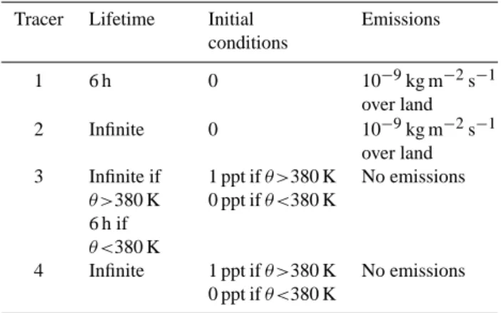
Table 1. Characteristics of the idealized tracers used in the
simula-tions.
Tracer Lifetime Initial conditions Emissions 1 6 h 0 10−9kg m−2s−1 over land 2 Infinite 0 10−9kg m−2s−1 over land 3 Infinite if θ >380 K 6 h if θ <380 K 1 ppt if θ >380 K 0 ppt if θ <380 K No emissions 4 Infinite 1 ppt if θ >380 K 0 ppt if θ <380 K No emissions
the stratosphere (see Table 1). The first one is a short-lived tracer designed to focus only on the effect of individ-ual convective events. Its lifetime of 6 h is long enough to be transported by convection but not to be significantly af-fected by large scale advection and diffusion. It is emitted only above land with an arbitrary constant emission rate of 10−9kg m−2s−1. It is initialized to 0. The second tracer has the same initial condition and same emission rate but an infinite lifetime in order to analyse TST at the regional scale. Finally, we used two stratospheric tracers to study the effect of convection on Stratosphere to Troposphere Trans-port (STT). The first one is initialized with a constant mixing ratio of 1 ppt for potential temperatures greater than 380 K (which corresponds approximately to the tropopause level in the tropics and is well into the TTL) and 0 below. Its life-time is infinite for potential temperatures greater than 380 K and 6 h below 380 K. The second has the same setup but its lifetime is infinite over the whole atmospheric column.
2.3 Convection closures and parameterizations
In the present paper, we test five convection closures plus one different convection parameterization and we analyse their impact on the troposphere-stratosphere transport (TST and STT) of tracers. Convection parameterization schemes are procedures that attempt to account for the collective effect of sub-grid scale convective processes on large-scale model variables. These effects (latent heating, evaporative cooling, generation of cirrus clouds associated with the anvil, etc.) have to be determined from the available model variables. Different cumulus parameterizations were developed during the last decades in order to improve model results in con-vective areas. The mass-flux approach is generally used in mesoscale models. It attempts to explicitly account for con-vective processes at each grid point by combining a cloud model with the assumption that convection acts to restore the stratified grid column based on moist parcel stability. The
cloud model estimates the properties of the convection. The closure assumption specifies the amount of convection that occurs in order to achieve the desired rate of stabilization.
Parameterizations used are based on the formulation pro-posed by Grell (1993) and Grell et al. (1994) and modi-fied by Grell and D´ev´enyi (2002) to allow the use of five different closure assumptions: Grell (called GR hereafter) (Grell, 1993), Arakawa Schubert (AS) (Arakawa and Schu-bert, 1974), Kain-Fritsh (KF) (Kain and Fritsch, 1992), moisture convergence (MC) (Kuo, 1974; Krishnamuti et al., 1983), and Low-Omega (LO) (Frank and Cohen, 1987). For each closure the same conceptual model is used; namely, the cloud consists of two steady state circulations caused by an updraft and a downdraft. There is no direct mixing between cloud air and environmental air except at the top and the bot-tom of the circulation. The additional convection parameter-ization used is based on an ensemble approach (EN) (Grell and D´ev´enyi, 2002).
The AS closure uses the quasi-equilibrium assumption which states that the stabilisation of the atmosphere by con-vection is in quasi-equilibrium with the destabilization by large scale processes. The GR closure is a modified AS clo-sure including moist convective-scale downdrafts. The KF closure also uses the stability closure but without any depen-dence with large scale motions leading to a pure instanta-neous stability closure. It assumes that a cloud can rise and then can instantly decay. Thus after subsidence calculations, the convection is supposed to build and to decay without a steady-state stage. The cloud properties are mixed horizon-tally with the subsided environment. The MC closure as-sumes that the convective activity is closely related to the total moisture convergence at the base of clouds. LO uses the same idea as MC, but introduces a downdraft forcing. This downdraft will cause additional mass-flux convergence, creating subsequent forcing of more convection. EN pro-vides the most probable solution based on statistical methods (Stephenson and Doblas-Reyes 2000) applied to a set of sen-sitivity calculations using perturbed values in GR, AS, KF, MC and LO parameters. The six simulations run using these parameterizations will be referred hereafter as GR, AS, KF, MC, LO and EN experiments.
3 Evaluation of the model meteorological fields
In the present study we cannot validate idealised tracers di-rectly using tracer measurements. Rather we evaluate the atmospheric dynamics by comparing meteorological fields provided by the six simulations against observations. For this purpose we used satellite rainfall estimates from TRMM (Tropical rainfall Measuring Mission), radisoundings and SCOUT-O3 aircraft measurements. In the Maritime con-tinent area, very few radiosoundings from the operational network provide reliable data. Therefore we only used radiosoundings launched in the frame of the SCOUT-O3
campaign from Darwin in Australia and those launched from Manus (see Fig. 1). Manus station operates in the frame of the ARM project (Atmospheric Radiation Measurement, http://www.arm.gov/). The comparison with the SCOUT-O3 aircraft measurements allows us to make a detailed analysis of the model behaviour on a case study.
3.1 Comparison with TRMM surface rainfall estimates
We compared the surface accumulated rainfall obtained with the six convection schemes to those estimated by TRMM. The dataset used is 3-hourly and 0.25◦×0.25◦resolution and
was produced by the 3B42 algorithm (Huffman et al., 2007, http://trmm.gsfc.nasa.gov). Figure 3a shows the daily mean surface rain rates (in mm day−1)estimated by TRMM during the one-month simulation period.
Almost all the domain experienced significant precipita-tion (over 0.1 mm day−1) except in three areas located South of 15◦S and North of 15◦N. We can also identify four ma-jor areas with high precipitation rates (above 10 mm day−1)
located
– over the New Guinea island (around 140◦E; 5◦S), with values reaching 10 to 20 mm day−1in the Southern part of the island.
– from the Eastern coast of the Malaysian peninsula
(around 100◦E; 10◦N) to the Eastern coast of Thai-land (110◦E; 12◦N), with very high values above 20 mm day−1
– over all the Indonesian Islands (from 100◦E to 115◦E; 0◦S to 30◦S)
– on the Eastern coast of Philippines (from 110◦E to 115◦E; 10◦N to 15◦N) with values reaching up to 20 mm day−1.
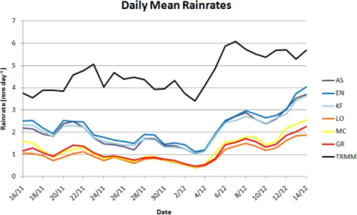
The TRMM 3B42 product is based on different satellite measurements mainly from passive remote sensing instru-ments. It leads to uncertainties on the surface rainrate esti-mates mainly over land and for very low rainrates. To assess the quality of this product for the chosen area and time pe-riod it was compared to the rainrate estimates provided by the Global Precipitation Climatology Project “One-Degree Daily Precipitation DataSet” product (GPCP, Huffman et al., 2001). The TRMM 3B42 product showed a very good agree-ment for both the precipitation location and intensity (not shown) giving confidence in the TRMM estimates used here. The simulation period takes place during the monsoon es-tablishment in the Maritime Continent region. Convective activity progressively grows from October to January. A complete description of the meteorological situation during the SCOUT-O3 period is provided in Brunner et al. (2009). Figure 2 displays the time evolution of daily mean rainrates averaged over the whole domain between the 16 November and the 14 December for TRMM measurements and for the
Fig. 2. Time evolution of the daily mean rainrate averaged over the
simulation domain in mm day−1.
six simulations. It shows the progressive enhancement of the precipitation from 3.8 mm day−1to 5.6 mm day−1, with a
large increase at the beginning of December. The 6 parame-terizations well represent the variability of precipitation with time but underestimate the rainrate values. Comparing the six model experiments we can class the convection closures into two groups providing similar results: AS, KF and EN in Group 1, and GR, MC and LO in Group 2. Group 1 provides results generally closer to TRMM measurements than Group 2.
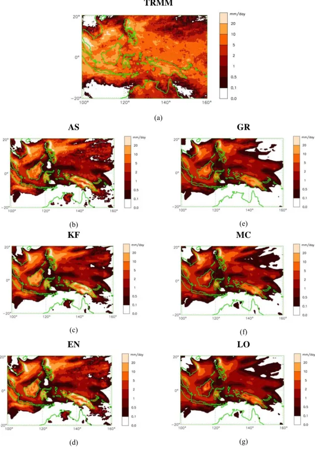
This result is consistent with the mean surface rainrates av-eraged over the whole simulation period (Fig. 3b to g). The six model experiments well locate the areas of high and low precipitation rates compared with the TRMM-based obser-vations. The very convective areas are well simulated by all six model simulations. Group 1 simulates more extended ar-eas of light precipitation in better agreement with TRMM. For high rainrates Group 1 is closer to the observations over Malaysia and Indonesian Islands around 20 mm day−1. On the other hand, the lower rates obtained with Group 2 are in better agreement with the measurements over New Guinea where TRMM estimates give values around 10 mm day−1 for the South of the island and 5 mm day−1 for the North. Group 1 tends to slightly overestimate the values from 1 to 5 mm day−1in this area. Group 1 simulations are also able to capture some of the convection occurring in the North of Australia around Darwin which is missed by Group 2. In other areas TRMM shows more precipitation than all the simulations especially in the centre and in the South over ocean. This could be partly related to a large uncertainty on light precipitation in 3B42 that possibly leads to an overes-timation of surface precipitation. But it is also likely due to an uncertainty in light precipitation prediction in the model in all simulations. This is confirmed by the distribution of the model surface rainrates versus TRMM displayed in Fig. 4. Both Group 1 and Group 2 show a tendency to un-derestimate low rainrates under 10 mm day−1 that are as-sociated to stratiform precipitation and to low convective
TRMM
(a)AS
(b)GR
(e)KF
(c)MC
(f)EN
(d)LO
(g)Figure 3. Mean surface rainrate in mm day
-1from 15 November 2005 to 15 December 2005
for (a) TRMM and the model simulations using (b) Arakawa-Schubert, (c) Kain-Fritsch, (d)
Ensemble, (e) Grell, (f) Moisture Convergence, (g) Low Omega.
- 33 -
Fig. 3. Mean surface rainrate in mm day−1from 15 November 2005 to 15 December 2005 for (a) TRMM and the model simulations using
(b) Arakawa-Schubert, (c) Kain-Fritsch, (d) Ensemble, (e) Grell, (f) Moisture Convergence, (g) Low Omega.
Figure 4. Distribution of model surface rainrate versus TRMM averaged over the whole
period for (a) Arakawa-Schubert, (b) Kain-Fritsch, (c) Ensemble, (d) Grell, (e) Moisture
Convergence, (f) Low Omega.
- 34 -
Figure 4. Distribution of model surface rainrate versus TRMM averaged over the whole
period for (a) Arakawa-Schubert, (b) Kain-Fritsch, (c) Ensemble, (d) Grell, (e) Moisture
Convergence, (f) Low Omega.
- 34 -
Figure 4. Distribution of model surface rainrate versus TRMM averaged over the whole
period for (a) Arakawa-Schubert, (b) Kain-Fritsch, (c) Ensemble, (d) Grell, (e) Moisture
Convergence, (f) Low Omega.
- 34 -
Figure 4. Distribution of model surface rainrate versus TRMM averaged over the whole
period for (a) Arakawa-Schubert, (b) Kain-Fritsch, (c) Ensemble, (d) Grell, (e) Moisture
Convergence, (f) Low Omega.
- 34 -
Figure 4. Distribution of model surface rainrate versus TRMM averaged over the whole
period for (a) Arakawa-Schubert, (b) Kain-Fritsch, (c) Ensemble, (d) Grell, (e) Moisture
Convergence, (f) Low Omega.
- 34 -
Figure 4. Distribution of model surface rainrate versus TRMM averaged over the whole
period for (a) Arakawa-Schubert, (b) Kain-Fritsch, (c) Ensemble, (d) Grell, (e) Moisture
Convergence, (f) Low Omega.
- 34 -
Fig. 4. Distribution of model surface rainrate versus TRMM averaged over the whole period for (a) Arakawa-Schubert, (b) Kain-Fritsch, (c)
Ensemble, (d) Grell, (e) Moisture Convergence, (f) Low Omega. precipitation (5–10 mm h−1). Nevertheless Group 1 performs slightly better. Group 1 also provides a distribution between 10 mm day−1and 20 mm day−1(convectively generated pre-cipitation) in better agreement with TRMM estimates than Group 2.
In order to analyse more objectively the simulation perfor-mances we calculated precipitation scores: Equitable Threat Score, Probability of detection and False alarm ratio. Eq-uitable Threat Score evaluates how well modelled raining events correspond to observed raining events, according for hits due to chance. Probability Of Detection tells us what fraction of the observed raining events is correctly
elled. False Alarm Ratio highlights the fraction of the mod-elled events that do not occur. Calculation methods and minimum/maximum values for these scores are displayed in Fig. 5a while results can be seen in Fig. 5b to d. Equitable Threat Score ranges from 0.45 to 0.65 showing the generally good behaviour of the model to forecast precipitation. This is related to the high Probability Of Detection (0.57 to 0.95) meaning that the model is able to trigger precipitation at the right place and time. It also provides fairly often precipi-tation where not observed (False Alarm Ratio∼0.3). Both Equitable Threat Score and Probability Of Detection evolves towards an improvement during the simulation period. This
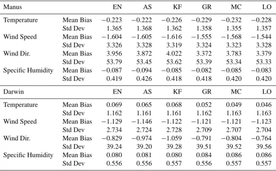
Table 2. Mean bias and standard deviation of bias for temperature (K), wind speed (m s−1) and direction (◦) and specific humidity (g kg−1) based on 12-hourly radiosounding done at Manus and Darwin during the whole simulation period.
Manus EN AS KF GR MC LO
Temperature Mean Bias −0.223 −0.222 −0.226 −0.229 −0.232 −0.228 Std Dev 1.365 1.368 1.362 1.358 1.355 1.357 Wind Speed Mean Bias −1.604 −1.605 −1.616 −1.555 −1.568 −1.544 Std Dev 3.326 3.328 3.319 3.324 3.323 3.328 Wind Dir. Mean Bias 3.956 3.872 4.022 3.372 3.783 3.379 Std Dev 53.79 53.45 53.62 53.39 53.34 53.33 Specific Humidity Mean Bias −0.087 −0.094 −0.085 −0.082 −0.085 −0.083 Std Dev 0.419 0.426 0.418 0.418 0.420 0.420
Darwin EN AS KF GR MC LO
Temperature Mean Bias 0.069 0.065 0.068 0.052 0.049 0.046 Std Dev 1.162 1.161 1.161 1.162 1.163 1.163 Wind Speed Mean Bias −1.129 −1.146 −1.122 −1.121 −1.121 −1.123 Std Dev 2.734 2.724 2.728 2.709 2.707 2.704 Wind Dir. Mean Bias −0.829 −0.974 −1.059 −0.791 −0.804 −0.764 Std Dev 39.24 39.20 39.28 39.51 39.52 39.56 Specific Humidity Mean Bias 0.080 0.081 0.080 0.084 0.086 0.086 Std Dev 0.556 0.556 0.557 0.556 0.557 0.557
shows that the model predicts better the precipitation loca-tion and triggering time in periods of more active convec-tion. The six parameterizations provide significant differ-ences only during the first two weeks when convection is relatively weak. This indicates that in a less convectively un-stable environment the behaviour of the 6 parameterizations differs more than in a more convective environment.
All these results show that the simulations are mainly dif-ferent by the amount of precipitation produced and can be sorted using this criteria in two groups. Group 1 (EN, AS, KF) gives results closer to observations than Group 2 (LO, MC, GR).
3.2 Comparison with radiosounding data
Comparisons were done with the 12-hourly radiosoundings launched from Darwin (130◦E; 12◦) during the field cam-paign of the SCOUT-O3 project and from Manus Island (147◦E; 2◦S) in the North of New-Guinea in the frame of the ARM program. Note that Manus location is interesting since this island is in an area where strong convective events are frequent as shown by the TRMM mean rainrate estimates which are above 5 mm day−1(see Fig. 3a).
Table 2 shows the mean bias (mean of model – mean of measurement) and the standard deviation of the bias for the six simulations for temperature, wind direction, wind speed and specific humidity. To calculate these statistics the ra-diosounding data were averaged over the model vertical lev-els. The 6 runs provide similar results for all parameters and a generally good agreement with the measurements. The
dif-ference in mean bias from one closure to another is not sig-nificant from a statistical point of view.
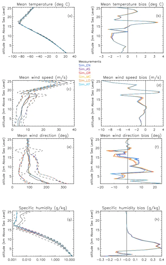
Figure 6 shows vertical profiles for the parameters listed in Table 1 only at the Manus station, since results for Dar-win station provide similar conclusions. The model re-sults for the 6 experiments are generally close and in good agreement with the radiosonde data for temperature and winds. Tropospheric temperatures show a mean warm bias of 1.5◦C. A larger positive bias is found around the cold point tropopause reaching 3◦C in the model simulations. The very
low tropopause temperatures observed in the Western Pacific are related to the intense convective activity in this area char-acterized by high-reaching cumulo-nimbus. Figures 6a and 6 show that the model is not able to cool enough around the cold point tropopause in the Manus area. This can be partly related to an underestimation of the convective activity in the model at Manus location (see Fig. 3) and partly to the model horizontal resolution (60 km) that cannot simulate the small scale impact of convection on temperature. The differences between the six simulations are negligible for most altitudes except in the 8–11.5 km range. In this range Group 1 results are slightly better compared to observations by about 0.3 K.
Both the simulated wind speed (Fig. 6c) and direction (fig 6e) are in good agreement with the measurements ex-cept above 23 km where the strong stratospheric winds are underestimated by the model. The mean bias for the wind speed is around 1 m s−1 below 16 km. In the 16–19.5 km range the model shows variations in the easterly wind inten-sity similar to the measurements but much less pronounced with a bias ranging between −5 to +4 m s−1. The wind
- 35 -
Fig. 5. Definition and minimum/maximum values of Equitable Threat Score, Probability Of Detection and False Alarm Ratio (a) and daily
evolution of (b) ETS, (c) POD and (d) FAR during the simulation period for the six closures.
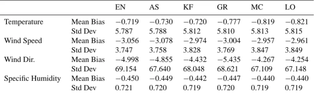
Table 3. Mean bias and standard deviation of the bias for the 6 aircraft flights (23rd, 25th and 29th of November, Falcon and Geophysica)
for temperature (K), wind speed (m s−1) and direction (◦) and specific humidity (g kg−1).
EN AS KF GR MC LO
Temperature Mean Bias −0.719 −0.730 −0.720 −0.777 −0.819 −0.821 Std Dev 5.787 5.788 5.812 5.810 5.813 5.815 Wind Speed Mean Bias −3.056 −3.078 −2.974 −3.004 −2.957 −2.961
Std Dev 3.747 3.758 3.828 3.769 3.847 3.849 Wind Dir. Mean Bias −4.998 −4.855 −4.432 −5.435 −4.267 −4.254
Std Dev 69.154 67.640 68.048 68.621 67.109 67.148 Specific Humidity Mean Bias −0.450 −0.449 −0.442 −0.447 −0.440 −0.440
Std Dev 0.721 0.720 0.719 0.720 0.719 0.719
direction presents a mean bias less than 20◦over the entire
atmospheric column. The radiosoundings data show that the tropopause region over Manus is marked by very strong gra-dients with a high vertical variability in both the dynamic
and the thermodynamical fields. These gradients are pro-duced by all six model simulations thanks to the fine vertical resolution used but smoothed. When comparing model sim-ulations to radiosounding data one has to keep in mind the
- 37 -
Figure 6. Com
parison between the Manus radios
ounding data and the six m
odel simulations:
(a and b) for tem
perature, (c and d) f
or horiz
ontal wind speed and (e a
nd f
) wind direction, (g
and h) for specific hum
idity. Left panels display
the m
ean (s
olid line
)
and standard deviation
- 38 -
Fig. 6. Comparison between the Manus radiosounding data and the six model simulations: (a, b) for temperature, (c, d) for horizontal wind
speed and (e, f) wind direction, (g, h) for specific humidity. Left panels display the mean (solid line) and standard deviation (dashed line) and right panels the mean bias (model minus observation). Black lines are for the radiosounding data and colored lines for the model simulations. The radiosounding data are averaged over the model vertical levels.
representativeness issue. Part of the observed gradients and variability may be linked to local effects (Manus Island being
∼100km long and ∼30 km wide) that cannot be captured by the model that uses a 60 km horizontal resolution. The com-parison between the six simulations shows differences on the wind speed and direction. For the wind speed (Fig. 6d) they are significant between 10 and 17 km altitude with a reduced bias for the Group 2 up to 0.5 m s−1. For the wind direction there are differences at nearly all the levels with a average mean bias of 8◦. As for the temperature and the wind speed, the six simulations can be sorted into the same two groups as defined in Sect. 3.1. Depending on the altitude range Group 1 is either better or worse than Group 2 compared to mea-surements.
The results for the specific humidity are displayed in Fig. 6g and h. Note that the humidity measurements in the upper troposphere and lower stratosphere should not be considered since they are expected to be not very reliable at very low temperatures and water vapor con-tents. In Fig. 3g the six model simulations overesti-mate the specific humidity above 4 km altitude. This can only partly be related to the known remaining small dry bias of the Vaisala RS92 data (Balloon-Borne Sounding System Handbook, http://www.arm.gov/publications/tech reports/handbooks/sonde handbook.pdf). The model simu-lations do not convert enough tropospheric moisture into pre-cipitation leading an overestimation of the water vapour mix-ing. This is consistent with the model underestimation of the low rainrates (see Sect. 3.1 and Fig. 3).
3.3 Comparisons with meteorological data from Falcon
and Geophysica flights
During the simulation period several DLR-Falcon and Geo-physica (M55) flights (9 for each aircraft) were done around Darwin (Australia), in the framework of the SCOUT-O3 field campaign (Vaughan et al., 2008; Brunner et al., 2009). Most of the flights were done around the Hector convective events regularly occurring over the Tiwi Islands. Some of them were extended flights planned for study of the surround-ing regions: survey flights on the 23rd, 25th, and the 29th November, remote sensing flight on the 5th December. Since the model simulations cover a large area, a comparison with the extended flights was preferred for the model evaluation. On the 5th December, aircrafts flew southward and a long part of the flight was done outside or close to the limits of our domain. Therefore this flight has not been used. The same remark applies for the beginning of the 29th November flight for which only legs done after 08:30 LT have been consid-ered. A statistical comparison of all the selected flights was done (Table 3). It shows higher differences between model and measurements than for the radiosounding comparison. This is due to the small number of selected fights and the fact that measurements were mainly done around the TTL alti-tude. Manus radiosounding results have highlighted that this
is the altitude where bias is the greatest. However, similar results were obtained for all six simulations with differences less than 15% (except for wind direction were difference is
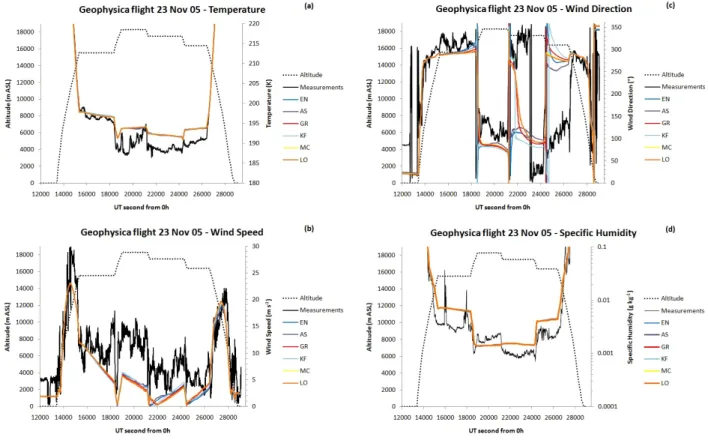
∼20%). To illustrate in more details the results we have chosen Falcon and Geophysica flights that took place on the 23rd November due to their large extents both in space and time. On this date the Geophysica aircraft and the Falcon performed coordinated flights whose objective was the de-tailed probing of the TTL over the Arafura Sea (see Fig. 1). Both Geophysica and Falcon flew long north-east oriented legs perpendicular to the mean flow expected to be north-westerly in the TTL. Flying back and forth along the same line twice, the Geophysica sampled around the cold point tropopause at four different levels: one significantly below the cold point level at ∼15.6 km (leg 1), two close to the cold point tropopause at ∼17.5 km (leg 3) and ∼16.4 km (leg 4), and one level well above at ∼18.3 km (leg 2). The flight paths are displayed in Fig. 14 in Brunner et al. (2009).
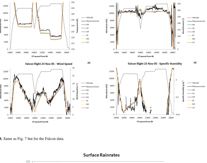
Figures 7 and 8 show the comparison between the results of the six simulations and the measurements collected re-spectively by the Geophysica and the Falcon instruments. Model temperatures are in good agreement with the mea-surements during the Geophysica ascent, leg 1 and the de-scent and to a lesser extend leg 2. For the two aircraft legs performed around the cold point tropopause level there is an overestimation of the temperature by the model of about 5◦C. The comparison with the Falcon temperature measure-ments shows that modeled temperatures around 12 km alti-tude are about 2◦C degrees lower than the aircraft measure-ments. This is consistent with the radiosounding compari-son showing that the model provides too warm temperatures around the cold point tropopause and too cold temperatures in the troposphere up to 14 km. There are no significant dif-ferences between the six simulations for the temperature for both Geophysica and Falcon flights.
The horizontal wind speed and wind direction simulated by the six runs along the aircraft trajectories are generally in good agreement with both the Geophysica (Fig. 7b and c) and the Falcon (Fig. 8b and c) measurements. In the cold point tropopause region (around 17 m altitude) the vari-ations of the wind velocity are well captured by the model compared to the Geophysica measurements but are under-estimated. This is consistent with the Manus radiosound-ing showradiosound-ing a strong increase of the wind speed near the tropopause that is underestimated by the model. The six model runs give very close results for the wind speed and the wind direction with differences of 2 m s−1and 6 degrees
at maximum which are much smaller than the differences be-tween each model simulation and the aircraft observations.
Specific humidity measurements aboard the Falcon air-craft are well simulated by the six model runs with a slight model overestimation for the aircraft leg at 12 km altitude (see Fig. 8d). This overestimation is much lower than that obtained in the comparison with the Manus radiosondes in-dicating that the Manus sondes likely underwent a significant
Fig. 7. Comparison between the Geophysica meteorological data and the six model simulations. (a) Temperature (K), (b) horizontal wind
speed (m s−1), (c) wind direction (◦) and (d) specific humidity (g kg−1). The black lines are for the aircraft measurements and the coloured lines for the model results. The dashed line is the model altitude in m.
dry bias in the upper troposphere. Modeled values are also in a fairly good agreement with the Geophysica measurements (Fig. 7d) but with an overestimation for all legs except leg 2 which was performed significantly above the cold point tropopause. This illustrates the fact that any of the convection parameterizations/closures used are able to modify signifi-cantly the specific humidity above the cold point tropopause from its initial smooth state provided by ECMWF analysis. Both the Falcon and the Geophysica measurements exhibit strong peaks over short time periods (e.g. around 16 000 and 18 000 s in the Geophyisica flight). CO measurements were also gathered on board the Geophysica aircraft during the flight. A comparison shows that the humidity peaks are cor-related with CO peaks indicating their link with deep convec-tion events. The six simulaconvec-tions use a horizontal resoluconvec-tion too coarse to capture these peaks that are very localized in space and time.
3.4 Conclusion and discussion on the meteorological
comparison
The simulations give results that are generally consistent with the radiosounding and aircraft meteorological data but
exhibit small differences between them. From these differ-ences it is not possible to get guidance on which convec-tion parameterizaconvec-tion is best. The surface rainrates given by Group 1 (EN, AS, KF) are significantly better than Group 2 (LO, MC and GR) for both low and heavy precipitation. This indicates that the AS, KF and EN parameterizations perform better than the other three closures.
In this study we use the Grell’s simple mass flux frame-work with different closure assumptions based on mass-flux parameterizations commonly used in mesoscale models. The five closure assumptions (GR, AS, KF, LO, MC) drive the modulation of convection by environment (noted dynamic control in Grell 1993). The Ensemble (EN) also takes into account statistically a variability of the modulation of the en-vironment by the convection and of the cloud model. The similarity of the EN to the AS and KF simulations means that dynamic control dominates the parameterization behaviour in the EN simulation. The model results clearly show that all closures or parameterizations tend to trigger convection at the same times and locations. The main difference between the 6 simulations is on the rainfall rate prediction which ex-hibits significant differences. Figure 9 shows the total and the convective rainfall rates from the 6 simulations averaged
Fig. 8. Same as Fig. 7 but for the Falcon data.
Figure 9. Total surface rainrate and convective surface rainrate provided by the convective scheme averaged over the simulation domain and period for the six closures. The number gives the ratio convective versus total in %.
- 44 -
Fig. 9. Total surface rainrate and convective surface rainrate provided by the convective scheme averaged over the simulation domain and
period for the six closures. The number gives the ratio convective versus total in %.
Fig. 10. Tracer volumic mixing ratio profiles (in ppbv) averaged
over the model domain and over the one month simulation period using 3-hourly model outputs for (a) Tracer 1 and (b) Tracer 2. The blue lines correspond to the EN simulation and the red lines to the GR simulation.
spatially and temporally and their ratio. Group 1 provides more precipitation, mainly through the convection parame-terization with almost ∼77% of the total precipitation. For Group 2 this is only ∼45%. For GR, LO and MC (Group 2), the lower convective precipitation is partially compensated by the production of rain by the microphysical parameteriza-tion but leading to lower total precipitaparameteriza-tion. Group 2 is less efficient at producing precipitation than Group1.
The effects of the different closures and parameterisations on the temperature, horizontal wind and specific humidity are significant locally but remain small on average since convec-tion parameterizaconvec-tion is not triggered at all grid points and for each timesteps. In convectively active areas such as Manus Island, there are differences in the meteorological parameters in the upper troposphere and in the TTL. This corresponds to the top of the deep convection circulation in the Grell’s framework where there is direct mixing between cloud air and environment air.
Fig. 11. Mean temperature (top panel) and potential temperature
(bottom panel) as a function of altitude for the EN simulation. The mean values are calculated as in Fig. 10. The green, brown and purple lines correspond respectively to the altitudes of the mean TTL bottom and cold point.
4 Analysis of the tracer transport
The analysis of the results showed that the EN, AS and KF simulations (Group 1) provide results for the tracer transport that are very close. GR, LO and MC runs (Group 2) give very similar tracer results that are different from Group 1. This is why the simulations shown and discussed hereafter are only EN and GR since they illustrate the Group 1 and Group 2 results, respectively.
4.1 Tropospheric tracers
Figure 10 shows the tracer mixing ratio profiles averaged over the model domain and over the one month simulation period using 3-hourly model outputs for Tracer 1 (6 h life-time) and Tracer 2 (infinite lifelife-time). We only focus on monthly means due to the fact that similar results are found at shorter timescales. To interpret these profiles we have
displayed the mean temperature and potential temperature profiles in Fig. 11. Note that in Fig. 11 only the profiles for the EN simulations are plotted since the GR results are very close to EN. The mean cold point tropopause (−82◦C) and the mean 380 K level are close and located at 17.3 km and 17.1 km altitude respectively. To locate the TTL we use here the definition proposed by Fueglistaler et al. (2009): TTL top is at the 70 hPa level (425 K) and TTL bottom is located above the levels of main convection outflow at the zero radia-tive level under all sky conditions (∼150 hPa, 355 K). This gives for the model simulations the TTL top at 18.9 km alti-tude and the TTL bottom at 14 km.
In Fig. 10 the shape of the mean mixing ratio profiles for both tracers is typical of convective areas. There are large values in the low troposphere, decreasing in the mid-troposphere and increasing in the upper mid-troposphere with a maximum value reached around 15 km altitude. Above there is a rapid decrease reaching very low values around 18 km. The EN parameterization provides for both tracers lower mean mixing ratios in the lower and mid troposphere and larger above ∼10 km than GR with a ratio of ∼2 for the maximum values around 15 km altitude. The GR closure gives more frequent convection outflows below 10 km than EN and significantly less transport above. Having a 6-hour lifetime Tracer 1 shows the local effect of convection and is only weakly affected by the model diffusion. This means that the EN convection parameterization is able to drive sig-nificant amount of surface tracers into the TTL with a ra-tio between the TTL bottom and the surface values of 2.2%. The GR closure is much less efficient with a ratio of 0.8% and with at least a factor of three less above the cold point tropopause. The Tracer 2 mean profile shows a maximum around 15 km as for Tracer 1. This means that the tracers lifted by convection in the TTL are not largely transported down during the following days while they travel into the model domain whatever closure or parameterization is used. Moreover since there are only very small differences in the large scale convergence between the EN and GR experiments the large differences in the tropospheric tracer transport can be attributed mainly to the convection parameterization used. Figure 12 displays for EN and GR simulations the merid-ian mean over the one month period for both tracers and the corresponding vertical velocity. The meridian mean is the average over the model latitudes (between 20◦S and 20◦N). The tracer with a 6 h lifetime (Tracer 1) indicates where the convective transport occurs since it is rapidly removed af-ter uplifting due to its lifetime. In the EN and GR simula-tions the vertical transport by convection of Tracer 1 occurs at the same longitudes, mainly around 112◦E and 143◦E. They correspond to emission areas (only islands in the simulation setup) with high vertical velocities where an intense convec-tive activity is modelled as well as observed (mainly Borneo around 112◦E and New Guinea around 143◦E). For Tracer 2 the maxima in the TTL for both EN and GR simulations are shifted westward compared to Tracer 1 and located in the
Table 4. Mean tracer fluxes at different levels averaged over the
model domain and over the one month simulation period using 3-hourly model outputs.
Altitude (km) Tracer 1 flux Tracer 2 flux (10−12kg m−2s−1) (10−12kg m−2s−1) EN GR EN GR 12 (below TTL) 3.92 0.82 97.27 57.86 14 (TTL bot-tom) 4.04 0.59 65.33 22.88
100◦E–120◦E longitude range. This indicates that a signifi-cant part of Tracer 2 mixing ratio that is firstly transported vertically from the low levels to the TTL around 143◦E (New Guinea) is then horizontally advected. It reaches west-ern longitudes where it adds to the high TTL mixing ratios lifted by local convection (mainly Borneo) and spread in lati-tudes (Fig. 13a and b) by anticyclonic circulation, both in the northern and southern hemisphere. The comparison between Fig. 13a and b with Fig. 13c and d also shows that the tracer meridian distribution in the mid troposphere is also different between Tracer 1 and 2. Therefore the geographical distri-bution of a long lifetime tropospheric tracer depends on both the locations where the main convection occurs and the large scale dynamics. This last process transports horizontally as well as mixes the tracer with its environment.
The major effect of the closure assumptions is on the vertical distribution since they drive the convective updraft and downdraft characteristics. Grell’s formulation gives en-hanced tracer amounts at the top of convection outflow. It is on average lower in GR than in EN. To quantify the trans-port the mean fluxes are calculated from the vertical wind and the tracer mixing ratio at two altitudes in the upper tro-posphere: below the TTL at the level of frequent couvec-tive outflow (12km) and at the TTL bottom level (14 km). The mean values are calculated averaging tracer fluxes from the 3-hourly outputs over the model horizontal domain at a given altitude. Results are reported in Table 4. The mean surface flux for the two tropospheric tracers that are only emitted over land is 0.182×10⁻⁹kg m−2s−1. At 12 km alti-tude and at the TTL bottom level, they are similar and around 4×10⁻¹²g m−2s−1, representing around 2.2% of the emis-sion flux above land. This flux is decreasing rapidly with altitude reaching negligible values at the cold point level and above. Tracer 1 having a very short lifetime, this means that the EN simulation predicts upward transport in the TTL by overshooting convection but mainly below the cold point dy-namical barrier. With the horizontal resolution used the EN simulation is not able to simulate small scale overshooting transport at very high altitude. It favours the slow radiative ascent as pathway for the tracers to reach the stratosphere from the TTL. For the GR simulations Tracer 1 fluxes are
Fig. 12. Meridian mean from EN simulation of (a) Tracer 1, (b) Tracer 2 and (c) vertical velocity. (d), (e) and (f) are respectively the same
plots but for the GR simulation. The mean is calculated from the one month period using the 3-hourly outputs.
Fig. 13. 15 km height mean of Tracer 2 from EN simulation (a) and GR simulation (b). Wind vector are over plotted. The mean is calculated
from the one month period using the 3-hourly outputs.
Fig. 14. Same as Fig. 10 but for Tracer 3 and 4 (stratospheric
trac-ers). The dark line is the mean vertical profile at the initial time of the simulation.
∼5–6 times lower at 12 and 14 km altitude than for the EN simulation. At the cold point level and above the fluxes are negligible as in EN simulation. This shows that the GR sim-ulation provides dynamical fields that are different from EN simulation when convection occurs. This has a large impact on the tracer distribution. Variations of the fluxes for Tracer 2 are similar with altitude to Tracer 1 but with higher absolute values. This means that the large scale radiative transport underwent above the cold point level by Tracer 2 in the EN simulation reinforces the upward tracer fluxes.
4.2 Stratospheric tracers
Figure 14 shows the mean mixing ratio profiles for Tracer 3 and 4 (idealised stratospheric tracer) averaged similarly to Tracers 1 and 2 in Fig. 10. The EN and GR parameterizations provide a similar shape with values close to 1 down to the top of the TTL layer (∼19 km altitude). There is a sharp decrease of the tracer mixing ratio below down to 17 km followed by a smoother decrease down to 15 km where it reaches zero. The comparison with the initial mean profile indicates that strato-spheric tracers are partly mixed with the TTL air. More than 0.4 ppt are found for Tracer 4 at the cold point tropopause level (17.3 km) showing that the model is able to transport significant amounts of stratospheric tracers below the dy-namical barrier of the cold point level. But the very low differences between the EN and GR results suggest that this mixing is likely driven by the subgrid-scale diffusion in the model rather than by the direct effect of the convection pa-rameterization. This is also consistent with the results on the tropospheric tracers showing that convection, even using the EN parameterization, hardly reach the cold point tropopause level.
5 Conclusion
Tracer transport by tropical deep convection can be well sim-ulated by cloud resolving models running with fine vertical and horizontal resolutions. Global CTMs use coarse hori-zontal and vertical resolution and the tracer transport by con-vection is known to be a large source of uncertainty in the spatial distribution of chemical species. We propose to use regional long-term simulations with a limited area model to fill the gap between the global CTMs and the cloud resolv-ing models. Simulations are done in tropical regions where deep convection plays a major role in the upward transport of tracers towards the lower stratosphere. The objective if these two papers is to evaluate long-duration regional simu-lations with the mesoscale model CATT-BRAMS with ideal-ized tracers as a tool to produce realistic tracer transport by tropical convection. In this paper, we analyse the impact of different deep convection parametrizations on the transport of idealised tracer in the TTL. For this purpose a simulation over a 60◦longitude x 40◦latitude domain in the Maritime Continent was run for one month during the period of the SCOUT-O3 aircraft campaign. It uses a 60 km horizontal grid spacing and a 300 m vertical grid spacing in the TTL. The Grell (1993) convection parameterization framework ex-tended by Grell and D´ev´enyi (2002) is used. It allowed us to test the impact on deep convection tracer transport of 5 differ-ent closures commonly used in the literature and an ensemble parameterization based on these 5 closures.
Since it is not possible to compare the idealised tracers with measurements there is no direct validation of the tracer fields from the model simulations. The choice of idealised tracers is justified by two reasons: (i) if we had used real instead of idealised tracers the comparison would depend largely in this case on the emissions that are poorly quan-tified in time and space and (ii) idealised tracers facilitate the analysis and understanding of the impact of convection pa-rameterizations or closures on tracer transport. We used an indirect evaluation of the tracer transport through the assess-ment of the meteorological fields. Comparisons were done with a series of radiosoundings launched from Manus Island and Darwin during the simulation period and with SCOUT-O3 aircraft data (mainly gathered around 12 and 15–18 km altitude). The model shows a good agreement with the mea-surements for temperature and wind speed/direction but un-derestimate the large variability observed within the TTL. The simulations show generally small differences compared one to another on average. They have a similar mean impact on the large-scale environment although significant effect is found locally. The comparison with the TRMM surface rain-rate estimates shows that the 6 parameterizations or closures trigger convection generally at the same locations and times but provides different surface rainrates. The six experiments exhibit two types of behaviours with AS, KF and EN closures giving significantly better results. They reproduce well rain-rates in deep convective areas and tend to underestimate less
light precipitation than the other 3 closures. From this, we conclude that the use of AS, KF and EN gives better results than the 3 other closures, because they reproduce better the observed rainrates.
The tracer transport is analysed using four idealised trac-ers (6 h lifetime and infinite lifetime tropospheric tractrac-ers and a infinite lifetime stratospheric tracer) for the EN and GR parameterizations that represent respectively the EN/AS/KF and GR/MC/LO behaviour. For both parameterizations the general shape of the mean profile for both tropospheric trac-ers is similar. There are large values near the surface, a general decrease up to 10-11km altitude, a relative maxi-mum around 15 km and a sharp decrease above. But the EN parameterization transport much larger amounts of tropo-spheric tracers than GR from the surface into the TTL (14 km to 18.9 km altitude). This clearly shows that although there are small changes on average on the meteorological variables between the two groups the tropospheric tracer transport is very different. The EN and GR simulations provide differ-ent intensity of the upward convective flux leading to a more efficient uplift of tracers in EN simulation. This is consis-tent with the analysis of the rainrate results showing a more efficient production if precipitation in EN linked to stronger convective ascents.
Even with the EN parameterization the transport above the cold point tropopause is low. This indicates that none of the parameterization or closure used in this study are able to sim-ulate significant overshooting convection at and above these altitudes in the model. Once the tracer emissions are lifted in the TTL above the emission areas by deep convection, they are redistributed horizontally by large scale circulation if they have a sufficient lifetime. In the EN simulation the major part of the infinite tracer amount is not transported down af-ter a few days below the TTL thanks to large scale slow as-cending motions. In the GR simulation, less tracers remain in the TTL. The stratospheric tracer is on average signifi-cantly mixed with the TTL air but does not reach the mid-troposphere. This mixing is probably linked to the model diffusion rather than to the convection parameterization.
The detailed comparison of the model results with the air-craft data from the Falcon and the Geophysica shows that the model is not able to simulate the local variations of the mete-orological variables that are likely linked to convective activ-ity. This is due to the 60 km horizontal resolution used in the simulations which does not allow the model to provide the small scale effects of convection that can be of importance in the tracer transport. The important issue of the model hori-zontal and vertical resolutions is the subject of part 2 of this series of two papers.
In this study, we only used the Grell’s formalism which provides, even with different closures, similar response to convective instability with modulations in the flux inten-sity. A complementary work could be done using mass-flux parameterizations based on a more detailed cloud model. Moreover, to go further in the analysis of the type of
simulations done in the present study, the use of real tracers such as carbon monoxide could be considered.
Acknowledgements. This work was supported by the European
integrated project SCOUT-O3 (GOCE-CT-2004-505390) and by the program LEFE/INSU in France (projects UTLS-tropicale and Tropopause 2009). This work was granted access to the HPC resources of CINES under the allocation 2008- c2008012536 made by GENCI (Grand Equipement National de Calcul Intensif). The TRMM data were provided by GSFC/DAAC, NASA and the Manus radiosounding data by the ARM program funded by the US Department of Energy. The Falcon meteorological data were provided by the DRL (Deutsches Zentrum f¨ur Luft- und Raumfahrt, Germany) and the Geophysica meteorological data by the CAO (Central Aerological Observatory, Russia) and MDB (Myasishchev Design Bureau, Russia). We acknowledge A. Protat and P. May from the BMRC (Bureau of Meteorology Research Center). CATT-BRAMS is a free software provided by CPTEC/INPI and distributed under the CC-GNU-GPL license.
Edited by: N. Harris
The publication of this article is financed by CNRS-INSU.
References
Arakawa, A. and Schubert, W. H.: Interaction of a cumulus cloud ensemble with the large-scale environment, Part I., J. Atmos. Sci., 31, 674–701, 1974.
Baray, J. L., Ancellet, G., Randriambelo, T., and Baldy, S.: Trop-ical cyclone Marlene and stratosphere-troposphere exchange, J. Geophys. Res., 104, 13953–13970, 1999.
Brunner, D., Siegmund, P., May, P. T., Chappel, L., Schiller, C., M¨uller, R., Peter, T., Fueglistaler, S., MacKenzie, A. R., Fix, A., Schlager, H., Allen, G., Fjaeraa, A. M., Streibel, M., and Harris, N. R. P., The SCOUT-O3 Darwin aircraft campaign: rationale and meteorology, Atmos. Chem. Phys., 9, 93–117, 2009, http://www.atmos-chem-phys.net/9/93/2009/.
Corti, T., Luo, B. P., de Reus, M., Brunner, D., Cairo, F., Ma-honey, M. J., Martucci, G., Matthey, R., Mitev, V., dos Santos, F. H., Schiller, C., Shur, G., Sitnikov, N. M., Spelten, N., Voss-ing, H. J., Borrmann, S., and Peter, T.: Unprecedented evidence for overshooting convection hydrating the tropical stratosphere, Geophys. Res. Lett., 35, L10810, doi:10.1029/2008GL033641, 2008.
Cotton, W. R., Pielke Sr., R. A., Walko, R. L., Liston, G. E., Tremback, C. J., Jiang, H., McAnelly, R. L., Harrington, J.-Y., Nicholls, M. E., Carrio, G. G., and McFadden, J. P.: RAMS 2001: Current status and future directions, Meteorol. Atmos. Phys., 82, 5–29, doi:10.1007/s00703-001-0584-9, 2003.
Deng, A., Seaman, N., L., Hunter, G. K., and Satuffer, D. R.: Eval-uation of interregional transport using the MM5-SCIPUFF sys-tem, J. App. Meteor. 43, 1864–1886, 2004.
Duncan, B. N., Strahan, S. E., Yoshida, Y., Steenrod, S. D., and Livesey, N.: Model study of the cross-tropopause transport of biomass burning pollution, Atmos. Chem. Phys., 7, 3713–3736, 2007, http://www.atmos-chem-phys.net/7/3713/2007/.
Folkins, I., Loewenstein, M. Podolske, J., Oltmans, S. J., and Prof-fitt, M.: A barrier to vertical mixing at 14 km in the tropics: Evi-dence from ozonesondes and aircraft measurements, J. Geophys. Res., 104(D18), 22095–22102, 1999.
Folkins, I., Bernath, P., Boone, C., Donner, L. J., Eldering, A., Lesins, G., Martin, R. V., Sinnhuber, B.-M., and Walker, K.: Testing convective parameterizations with tropical mea-surements of HNO3, CO, H2O, and O3: Implications for
the water vapour budget, J. Geophys. Res., 111, D23304, doi:10.1029/2006JD007325, 2006.
Franck, W. M. and Cohen, C.: Simulation of tropical convective systems. Part 1: A cumulus parameterization, J. Atmos. Sci., 44, 3787–3799, 1987.
Freitas, S. R., Longo, K. M., Silva Dias, M. A. F., Chatfield, R., Silva Dias, P., Artaxo, P., Andreae, M. O., Grell, G., Rodrigues, L. F., Fazenda, A., and Panetta, J.: The Coupled Aerosol and Tracer Transport model to the Brazilian developments of the Re-gional Atmospheric Modeling System (CATT-BRAMS). Part 1: model description and evaluation, Atmos. Chem. Phys., 9, 2843– 2861, 2009, http://www.atmos-chem-phys.net/9/2843/2009/. Fueglistaler, S., Wernli, H., and Peter, T.: Tropical
troposphere-to-stratosphere transport inferred from trajectory calculations, J. Goephys. Res., 109, D03108, doi:10.1029/2003JD004069, 2004. Fueglistaler, S., Dessler, A., Dunkerton, T. J., Folkins, I., Fu, Q., and Mote, P. W.: The tropical tropopause layer, Rev. Geophys., 47, RG1004, doi:10.1029/2008RG000267, 2009.
Gevaerd, R. and Freitas, S.: Estimativa operacional da umidade do solo para iniciao de modelos de previso numrica da atmosfera. Parte 1: descrio da metodologia e validao, Brazilian Journal of Meteorology, LBA Special Issue, 21, 1–15, 2006.
Gettelman, A. E. and de F. Forster, P. M.: A climatology of the trop-ical tropopause layer, J. Meteor. Soc. Jpn., 80, 911–942, 2002. Gilliland, A. B. and Hartley, D. E.: Interhemispheric transport
and the role of convective parameterizations, J. Geophys. Res., 103(D17), 22039–22045, 1998.
Grell, G. A.: Prognostic evaluation of assumptions used by cumulus parameterizations, Mon. Weather Rev., 121, 764–787, 1993. Grell, G. A. and D´ev´enyi, D.: A generalized approach to
parame-terizing convection combining ensemble and data assimilation, Geophys. Res. Lett., 29, 1693, doi:10.1029/2002GL015311, 2002.
Grell, G. A., Dudhia, J., and Stauffer, D. R.: A description of the fifth-generation Penn State /NCAR mesoscale model, Tech. Note, NCAR/TN-398+STR, Natl. Cent. Atmos. Res., 138 pp., 1994.
Hack, J. J.: Parameterization of moist convection in the National Center for Atmospheric Research community climate model (CCM2), J. Geophys. Res., 99, 5551–5568, 1994.
Harrington, J. Y.: The effects of radiative and microphysical pro-cesses on simulated warm and transition season Arctic stratus, PhD Diss., Atmospheric Science Paper No. 637, Colorado State University, Department of Atmospheric Science, Fort Collins,