Structure of mass and momentum fields over a model aggregation of benthic filter feeders

(1)

HAL Id: hal-00297872

https://hal.archives-ouvertes.fr/hal-00297872

Submitted on 9 Feb 2007

HAL is a multi-disciplinary open access

archive for the deposit and dissemination of sci-entific research documents, whether they are pub-lished or not. The documents may come from teaching and research institutions in France or abroad, or from public or private research centers.

L’archive ouverte pluridisciplinaire HAL, est destinée au dépôt et à la diffusion de documents scientifiques de niveau recherche, publiés ou non, émanant des établissements d’enseignement et de recherche français ou étrangers, des laboratoires publics ou privés.

Structure of mass and momentum fields over a model

aggregation of benthic filter feeders

J. P. Crimaldi, J. R. Koseff, S. G. Monismith

To cite this version:

J. P. Crimaldi, J. R. Koseff, S. G. Monismith. Structure of mass and momentum fields over a model aggregation of benthic filter feeders. Biogeosciences Discussions, European Geosciences Union, 2007, 4 (1), pp.493-532. �hal-00297872�

(2)

BGD

4, 493–532, 2007

Mass and momentum fields over filter

feeders J. P. Crimaldi et al. Title Page Abstract Introduction Conclusions References Tables Figures ◭ ◮ ◭ ◮ Back Close

Full Screen / Esc

Printer-friendly Version Interactive Discussion

EGU Biogeosciences Discuss., 4, 493–532, 2007

www.biogeosciences-discuss.net/4/493/2007/ © Author(s) 2007. This work is licensed under a Creative Commons License.

Biogeosciences Discussions

Biogeosciences Discussions is the access reviewed discussion forum of Biogeosciences

Structure of mass and momentum fields

over a model aggregation of benthic filter

feeders

J. P. Crimaldi1, J. R. Koseff2, and S. G. Monismith2

1

Department of Civil and Environmental Engineering, University of Colorado, Boulder, CO, 80309-0428, USA

2

Department of Civil and Environmental Engineering, Stanford University, Stanford, CA, 94305-4020, USA

Received: 18 January 2007 – Accepted: 19 January 2007 – Published: 9 February 2007 Correspondence to: J. P. Crimaldi (crimaldi@colorado.edu)

(3)

BGD

4, 493–532, 2007

Full Screen / Esc

EGU Abstract

The structure of momentum and concentration boundary layers developing over a bed of Potamocorbula amurensis clam mimics was studied. Laser Doppler velocimetry (LDV) and laser-induced fluorescence (LIF) probes were used to quantify velocity and concentration profiles in a laboratory flume containing 3969 model clams. The model

5

clams incorporated passive roughness, active siphon pumping, and the ability to filter a phytoplankton surrogate from the flow. Measurements were made for two crossflow velocities, four clam pumping rates, and two siphon heights. The simultaneous use of the LDV and LIF probes permits direct calculation of scalar flux of phytoplankton to the bed. The results show that clam pumping rates have a pronounced effect on a range

10

of turbulent quantities in the boundary layer. In particular, the vertical turbulent flux of scalar mass to the bed was approximately proportional to the rate of clam pumping.

1 Introduction

Shallow estuaries are commonly inhabited by benthic communities of suspension feed-ers that filter phytoplankton and other particles from the overlaying flow. The extent to

15

which these feeders can effectively filter the bulk phytoplankton biomass depends on the vertical distribution and flux of phytoplankton in the water column. Phytoplankton generally reproduce near the surface where there are higher levels of incident light. Density stratification or low levels of vertical mixing can isolate phytoplankton in the up-per layers of the water column (Koseff et al.,1993). On the other hand, turbulent mixing

20

processes can distribute phytoplankton throughout the water column, where they be-come accessible to benthic grazers. But grazing acts as a near-bed sink of phytoplank-ton, and, in the absence of sufficient phytoplankton replenishment from above through mixing, can produce a phytoplankton-depleted near-bed region called a concentration boundary layer (O’Riordan et al.,1993). The severity of this concentration boundary

25

(4)

BGD

4, 493–532, 2007

Full Screen / Esc

EGU and the rate at which phytoplankton is fluxed to the bed by turbulent mixing processes.

The nature of the turbulence, and hence of the vertical mixing, depends on tidal en-ergy, waves, bed geometry, and the presence of the benthic feeders themselves, whose roughness and siphonal currents can alter the flow.

In the present study, we investigate how aggregations of benthic suspension feeders

5

can alter the structure of both the overlaying momentum and concentration fields. The physical roughness associated with benthic communities alters the turbulent velocity field above them (Butman et al.,1994;van Duren et al.,2006), significantly enhancing both turbulence intensities and Reynolds stresses. Active siphonal currents associ-ated with filter feeding also impact the overlaying flow structure (Ertman and Jumars,

10

1988;Larsen and Riisgard,1997), and have been shown to enhance turbulence inten-sities (Monismith et al.,1990;van Duren et al., 2006). The presence of suspension feeders also changes the structure of the concentration field above them through two mechanisms. First, near-bed concentrations are reduced by the filtering action of the community. Second, the alteration of the momentum field by both physical roughness

15

and siphonal pumping changes the rates at which phytoplankton and other particles are mixed by turbulence.

We use model aggregations of the Asian clam Potamocorbula amurensis for this study. San Francisco Bay in California, USA is abundantly populated by this invasive species (Carlton et al., 1990), and it has become clear that the grazing pressure

ex-20

erted by these clams alters the dynamics of phytoplankton blooms in the San Francisco Estuary. The goal of the study is to quantify changes to the momentum and concentra-tion fields produced by the passive siphon roughness and active siphonal pumping of the clam aggregations.

(5)

BGD

4, 493–532, 2007

Full Screen / Esc

EGU 2 Methods

2.1 Flume

The experiments were performed in an open channel recirculating flume in the Envi-ronmental Fluid Mechanics Laboratory at Stanford University. The flume is constructed of stainless steel and Plexiglas, with glass sidewalls in the test section to minimize

5

laser refraction at the glass/water interface. The flume capacity in normal operation is approximately 8000 liters. A centrifugal pump commanded by a digital frequency controller draws water from a downstream reservoir and charges a constant-head tank upstream of the flume (an overspill pipe returns excess water from the constant-head tank back to the downstream reservoir). Water from the constant-head tank enters the

10

flume through a full-width diffuser and then passes through three stilling screens with decreasing coarseness to remove any large-scale structure in the flow and homogenize the turbulence. The flow then passes through a 6.25:1 two-dimensional contraction and enters a rectangular channel. A 3 mm rod spanning the flume floor at the beginning of the channel section trips the boundary layer 2 m upstream of the test section. The

15

flow passes through the test section, then through an exit section, and finally over an adjustable weir back into the downstream reservoir. Freestream velocities in the test section of 10 cm/s to 40 cm/s are used for this study.

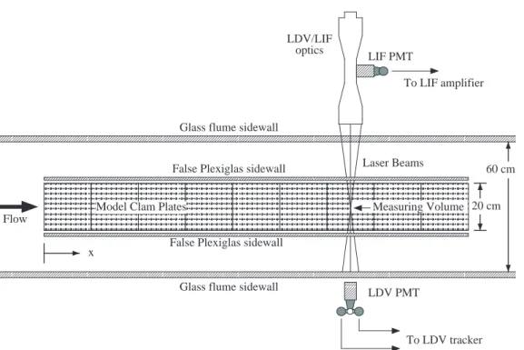
A top view of the flume test section is shown schematically in Fig.1. The test section is 3 m long and 0.6 m wide, with a rectangular cross section and a nominal flow depth of

20

25 cm. In the middle of the test section floor is a 1.8 m long by 20 cm wide removable section that can accommodate either a set of model clam plates or a single smooth plate for baseline flow measurements. A pair of thin Plexiglas sidewalls border the lateral edges of the model clam plates. These false walls extend vertically from the bed through the free surface and act as symmetry planes to effectively model a wide

25

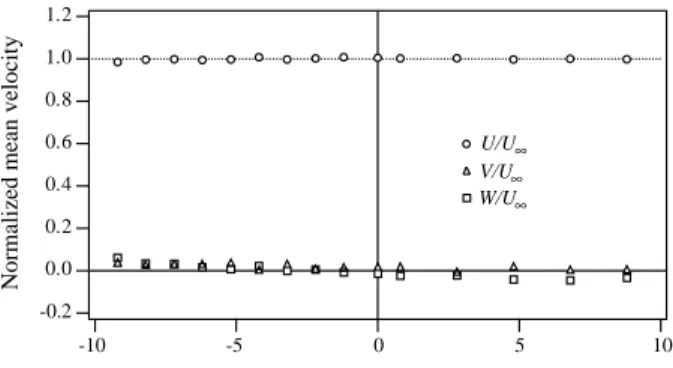
bed of clams. The boundary layers developing on the false vertical walls grow to only about 1 cm thick at the downstream edge, and thus have a minimal effect on the flow over the plates. Lateral profiles of normalized mean velocity within the false sidewalls

(6)

BGD

4, 493–532, 2007

Full Screen / Esc

EGU are shown in Fig.2.

These profiles were made in the freestream at a height of_{z=15 cm, over a smooth} bed. The false sidewalls are located 10 cm to each side of the flume centerline. The flow is seen to be quite uniform across the inner test section, with no significant varia-tion or secondary flow structure.

5

Measurements for this study were made on the flume centerline over the model clam plates (or over a smooth plate for baseline measurements). The streamwise location of the measurements is deonted byx, which is measured from the upstream edge of the plates, as shown in Fig. 1. The plates extend fromx=0 at the upstream edge to x=180 cm at the downstream edge.

10

2.2 Model clams

Models of clam aggregations were placed in the removable floor section of the flume. The models mimiced three clam feautures: (1) the physical roughness associated with siphons that are raised into the flow, (2) the incurrent and excurrent siphonal flows associated with filter feeding, and (3) the ability for the clams to filter mass from the flow.

15

Two types of the clam models were built, one with raised siphons (which were therefore rough) and one with flush siphons (which were smooth except for the presence of the siphon orifices). Tests were run with only one type of clam model (siphons raised or siphons flush) present in the flume at one time. Each model type consisted of nine identical 20 cm×20 cm square plates that fill the 1.8 m long cutout in the flume

20

floor. Each plate contains a 21×21 array of individual clam siphon pairs, resulting in 441 clams per plate, and a total of 3969 clams in the strip of nine plates. The clam models, while idealized, are full-scale representations of their biological counterparts, with regard both to siphonal dimension and pumping rates. The dimensions and flow rates were based on observations of real Potamocorbula amurensis clams made by

25

Cole et al.(1992) and Thompson (personal comm.).

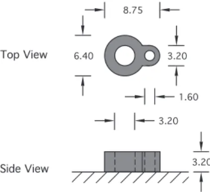
A schematic of an individual clam model with a raised siphon is shown in Fig.3. The incurrent and excurrent orifices (with diameters of 3.2 mm and 1.6 mm, respectively)

(7)

BGD

4, 493–532, 2007

Full Screen / Esc

EGU are visible as white circles in the top view. The side view shows that the raised siphon

models protrude 3.2 mm into the flow. For all tests reported in this study, flow was from left to right in the orientation shown in the figure. The clam models with flush siphons had the same incurrent and excurrent orifice geometry, but did not protrude into the flow. Thus, the flush siphon model for an individual clam consisted simply of a pair of

5

holes in a smooth plate through which siphonal currents flowed.

Models of individual clams are arrayed on plates that are placed in the flume test section. The geometry of the arrays is shown in Fig. 4, which illustrates the spacing between adjacent clams. This geometry is repeated across the entire array of 3969 clam models for both the raised and flush siphon model types.

10

The model clam plates were cast in a mold using a firm rubber; details of the con-struction process are given byO’Riordan(1993). The interior of the plates included a series of channels that linked all of the incurrent siphons together and all of the excur-rent siphons together. The back of each plate had a pair of outlets: one for all incurexcur-rent siphons, and one for all excurrent siphons. In practice, the incurrent and excurrent flows

15

were not completely uniform across the plate. In general, the clams near the center of the plate (where the plumbing was attached) had slightly higher flowrates than clams near the edge of the plate (due to frictional losses in the internal channels). Also, ir-regularities in the casting process led to variations in the flowrates of individual clams. While this was not an intentional feature of the design, it is likely more representative of

20

the real-world situation. For the sake of repeatability, measurements were made over an area of the clam plates where the pumping rates were quite uniform from clam to clam.

Filter feeders inhale phytoplankton-laden fluid through their incurrent siphons and then exhale fluid with some fraction of the phytoplankton removed through their

excur-25

rent siphons. Thus, while the volume of water entering and leaving the clam is constant, the amount of suspended scalar mass (e.g. phytoplankton) is not. We model this con-centration change by labeling the excurrent flows with a fluorescent dye. The model clams inhale ambient water from the flume, but they exhale water that has a known

(8)

BGD

4, 493–532, 2007

Full Screen / Esc

EGU concentration of dye. Thus, in our system, clear fluid respresents

phytonplankton-laden water in the real system, and dyed fluid respresents water in the real system that has had phytoplankton filtered from it. This inverse system, which was first used by Monismith et al.(1990) and then later byO’Riordan(1993) is advantageous because smaller amounts of dye are used.

5

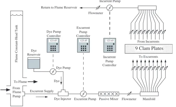
Figure 5 is a schematic representation of the plumbing system used to produce siphonal currents and to add dye to the excurrent flows. The bottom half of the figure is the excurrent system, and the top half is the incurrent system. The excurrent flows consist of ambient flume fluid with with a dose of dye added to it. This dosing pro-cess is done continually in real-time as the experiment is conducted. An electronically

10

controlled centrifugal pump draws ambient fluid from the flume’s constant-head tank into the excurrent supply line. The fluid in the constant-head tank is well-mixed and has the same background dye concentration as the fluid which is about to enter the flume. An electronically controlled gear pump then pumps concentrated dye from a 20-liter reservoir into to the excurrent stream. The concentrated dye enters the excurrent

15

stream via the dye injector, and is then mixed into the excurrent supply first by pass-ing through the centrifugal excurrent supply pump, and then through an in-line static mixer. A flowmeter measured the total excurrent supply flowrate, and a manifold then split the supply into nine streams. Individual flowmeters ensured that the nine streams had equal flowrates. Each of the nine streams passes into one of the nine model clam

20

plates, where a series of internal channels routes the excurrent fluid to each one of the 441 excurrent jets in each plate. Note that a small portion of the excurrent stream is diverted to the calibration jet for use as a reference for calibrating the LIF probe, as described later.

The incurrent flows are generated by a similar system, except that there is no dye

25

injection. An electronically controlled centrifugal pump draws fluid in through the in-current siphon orifices while nine flowmeters ensure that each of the nine model clam plates has the same incurrent flow rate. A manifold then combines the nine incurrent streams, and the resulting stream returns back into the flume reservoir downstream

(9)

BGD

4, 493–532, 2007

Full Screen / Esc

EGU of the flume test section. There is a great deal of turbulence in the flume reservoir

(generated by the plunging action of the flume flow spilling over the weir), and this tur-bulence constantly mixes the fluid in the reservoir. The reservoir therefore serves as a well-mixed source of fluid for the flume pump and the excurrent supply pump.

The concentration of background dye in the flume grows with time due to the constant

5

dosing of the excurrent flows. The system is designed such that this concentration growth is extremely linear in timeCrimaldi (1998). The excurrent flows contain a fixed amount of dye added on top of the existing background flume concentration, so the difference between the background concentration and the the excurrent concentration remains constant with time.

10

2.3 Instrumentation

2.3.1 Velocity measurements

A Dantec two-component laser-Doppler velocimeter (LDV) was used to measure ve-locities. This instrument was operated in tandem with a laser-induced fluorescence (LIF) probe to measure concentration fluxes, as described later. The LDV was driven

15

with an argon-Ion laser which was operated in the 514.5 nm single-line mode, with a nominal output of 1 Watt. The measuring volume is elliptical in shape, with the long axis oriented in the cross-channel direction. The dimensions of the measuring volume (to the e−2intensity contour) are approximately 0.1 mm in the vertical and streamwise directions, and 1 mm in the cross-channel direction. The smallest scales of motion

20

in the flows measured in this study can be determined by estimating the Kolmogorov scale as (Tennekes and Lumley,1972)

η_K ≈ κzν

3 u3_τ

!1₄

(1) whereκ is the Kolmogorov constant, z is distance from the bed, ν is the viscosity, and uτis the shear velocity. The smallest value ofηK for the flows in this study

(10)

BGD

4, 493–532, 2007

Full Screen / Esc

EGU ing touτ=1.7 cm/s and z=0.1 cm) is approximately 0.1 mm. Although this value of ηK is

comparable to the dimension of the measuring volume in the vertical and streamwise directions, it is smaller than the dimension in the cross-flow direction. Nonetheless, the LDV easily captures the larger scales responsible for the transport of mass and mo-mentum. The LDV laser and optics were mounted on a motorized, computer-controlled

5

three-axis traverse which permitted the LDV measuring volume to be positioned any-where within the test section. The traverse system was accurate to within approxi-mately 200 microns.

For validation purposes, LDV measurements of boundary layer turbulence were taken in the flume over a smooth plate that was installed in the same location where

10

the model clam plates were later installed. The LDV results were then compared with direct numerical simulations (DNS) of boundary layer turbulence over a smooth bed bySpalart (1988). Data were recorded at 23 logarithmically-spaced vertical stations between _{z=0.7 mm and z=180 mm, measured from the bed. Approximately 20 min} of velocity data were recorded at each station, at a sample rate of 80 Hz. The mean

15

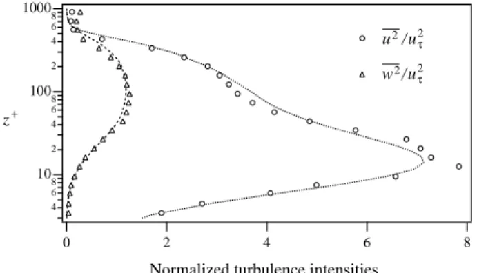
freestream velocity was U∞=11.6 cm/s, which resulted in a calculated momentum-thickness Reynolds number of Re_θ_{=1320. We compared the data to Spalart’s DNS} results simulated at Re_θ=1410. Although the Reynolds numbers differ by 6%, the vari-ation of normalized turbulence parameters with Re_θ is quite weak, enabling a valid comparison.

20

Normalized turbulence intensities derived from the LDV measurements over the smooth plate are shown in Fig. 6, along with the DNS results from Spalart (1988). The intensities are normalized by the square of the shear velocityuτ which was

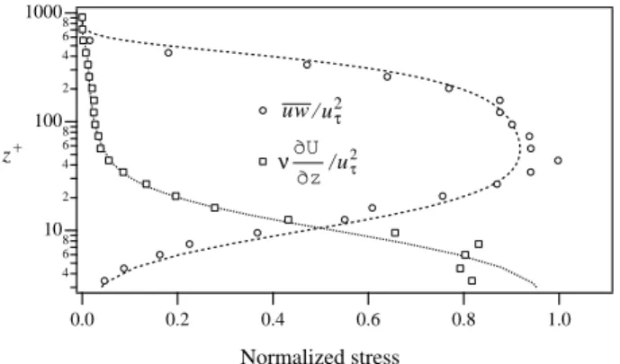
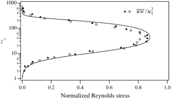
ob-tained by fitting the mean velocity profile to the law of the wall. Normalized turbulent and viscous stress profiles derived from the LDV measurements are shown in Fig.7

25

along with DNS results for comparison. The agreement between the LDV and DNS results is excellent for both the turbulence intensities and the stress profiles.

(11)

BGD

4, 493–532, 2007

Full Screen / Esc

EGU 2.3.2 Concentration measurements

We developed a laser-induced fluorescence (LIF) probe to make non-intrusive mea-surements of dye concentrations in the flow above the model clam beds. The LIF probe uses the same measuring volume as the LDV, ensuring that the velocity and concentration measurements are being made in the same location. This is particlarly

5

important for the scalar flux measurements, which result from correlations of velocity and concentration measurements. The laser light in the combined LDV/LIF measuring volume is absorbed by fluorescent dye in the flow and re-emitted at a different wave-length. The fluoresced light is optically filtered and converted to a electrical current with a photomultiplier tube (PMT). Finally, the current is converted to a voltage using

10

an ideal current-to-voltage converter.

Because the dye fluoresces in an omni-directional pattern, we were able to place the LIF receiving optics in the backscatter configuration without any loss of signal (as opposed to the LDV receiving optics, which were placed preferentially in the strong forward-scatter lobes). The LIF receiving optics and the LIF PMT were mounted directly

15

within the LDV front optics (using a backscatter module intended for making backscatter LDV measurements). Thus, the receiving optics for the LIF automatically moved with the measuring volume as the LDV/LIF system was traversed throughout the test section of the flume, maintaining a consistent alignment. The PMT for the LIF had a pinhole section that masked stray light which originated from anywhere other than the test

20

section. More details on the construction and operation of the LIF probe are given by Crimaldi(1998).

The smallest scalar fluctuations in a flow occur at the scale at which viscous diffusion acts to smooth any remaining concentration gradients. Batchelor (1959) defines this scale as

25

η_B = ηKPr−1/2 (2)

where Pr is the Prandtl number. According toBarrett (1989), the Prandtl number for Rhodamine 6G, the dye used in the study, is 1250. Therefore, the smallest

(12)

concentra-BGD

4, 493–532, 2007

Full Screen / Esc

EGU tion scalesη_B=3 microns are about 35 times smaller than the smallest scales of motion

ηK. Thus, the LIF probe cannot measure the smallest scales of motion present in the

studied flows. However, the LIF probe can easily measure the larger concentration scales that are responsible for the vast majority of the scalar flux.

To validate the LIF probe, we measured known dye concentrations in the

poten-5

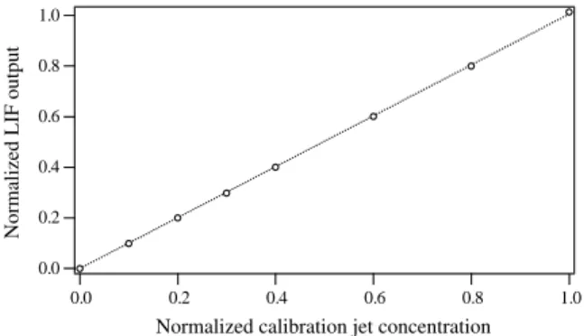
tial core of a jet flowing from a 7.5 mm diameter calibration tube within the flume test section. LIF measurements of the jet fluid were made 1 mm downstream of the jet orifice (_{x/D=0.13) which ensured that the measuring volume was well within the} po-tential core of the jet. Eight different dye concentrations ranging from 0 to 100 ppb were pumped through the jet, and the linearity of the resulting LIF data is shown in Fig.8.

10

The calibration jet concentrations are normalized by the maximum value used in the test (100 ppb). The LIF output is normalized so that the output from the 40 ppb jet is 0.4. Also shown in the figure is a linear fit to the LIF data. The least-squares estimate of the slope of the line is 1.006±0.003. The actual dye concentrations used in the mea-surements over the model clams rarely exceeded 5 ppb, well within the demonstrated

15

range of linearity of the LIF probe. The time response of the LIF probe is extremely fast; the time constants associated with the dye fluorescence, with the PMT, and with the LIF signal amplifier are extremely small relative to the time scales of turbulent motion in this flow.

During experiments over the model clams, the LIF calibration jet remained in the

20

flume, positioned above the measurement region in the freestream of the flow. A small portion of the dyed flow mixed for the excurrent supply was diverted through the cali-bration jet. The LIF probe was periodically positioned in the freestream and behind the calibration jet during experiments to maintain the probe calibration as background and excurrent concentrations rose during the experiments due to dye accumulation in the

25

(13)

BGD

4, 493–532, 2007

Full Screen / Esc

EGU 2.3.3 Concentration normalization

As discussed earlier, a known concentration of dye is continuously added to the excur-rent jets. The dyed fluid represents filtered fluid that is devoid of phytoplankton, and fluid without dye (other than the background dye) represents phytoplankton-laden fluid. Using the LIF probe, we calculate a nondimensional concentration in this “inverse”

5 system as C∗ inv= C − C_B CE−CB , (3)

whereC is the output of the LIF probe at the measurement location, CB is the

out-put due to the background dye (measured in the freestream), andC_E is the output of pure excurrent fluid (measured using the calibration jet). To put this “inverse”

measure-10

ment in a more intuitive framework, we then define a complementary nondimensional concentration

C∗

= 1 − C∗

inv (4)

such that C∗

=1 now corresponds (in the real system) to fluid with full phytoplankton load, andC∗=0 corresponds to fluid that has had its phytoplankton removed by

filtra-15

tion. These nondimensional concentrations could be converted to dimensional con-centrations for a real system by considering the ambient phytoplankton concentration and the filtering efficiency of the bivalve.

3 Results

Vertical profiles of velocity and concentration data were taken for two crossflow

ve-20

locities and four clam pumping rates, for each of the two clam model types (siphons flush and siphons raised). A summary of the experimental parameters that were varied during the profile measurements is given in Table1. For each vertical profile, simultane-ous LDV and LIF data were acquired at approximately 20 vertical stations. The stations

(14)

BGD

4, 493–532, 2007

Full Screen / Esc

EGU were logarithmically spaced, usually starting atz=0.5 mm, and ending at z=120 mm.

Typically, 100 000 samples of data were acquired at approximately 80 Hz from each LDV channel and from the LIF probe for each vertical station, although shorter records were used near the edge of the boundary layer where the variance of the signals was small.

5

The results presented in this paper focus on perturbations made to the momentum and scalar concentration fields by the presence of the clams. These perturbations come from two sources: the presence of roughness (in the case of the model clams with raised siphons), and the presence of siphonal currents and filtering. The flush siphonal orifices without clam pumping did not alter the flow, as is demonstrated in

10

Figs.9and10.

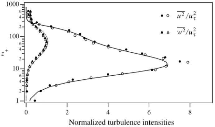
The data shown in these two figures compares the boundary layer flow over a smooth plate with the flow over the flush clam models, with no siphonal currents. Both exper-iments were performed with a freestream velocity of U∞=10 cm/s, corresponding to Reθ=560. Figure9 shows normalized turbulence intensities, and Fig. 10 shows

tur-15

bulent Reynolds stresses. The closed symbols represent the smooth plate data, and the open symbols represent the flush model clam data. The lines are DNS results by Spalart(1988) at Reθ=670. The results show that the flow over the flush siphon orifices

was indistinguishable from the flow over the smooth plate. Thus, the perturbations to the flow demonstrated later are due only to the presence of siphon roughness and/or

20

siphonal pumping.

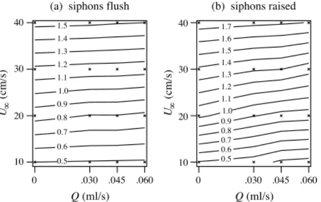
The effects of siphon roughness and pumping on the shear velocity are shown in Fig. 11. The shear velocity u_τ is a measure of the bed shear stress τ_w, where uτ=(τw/ρ)1/2. Contours ofuτ are shown as a function of freestream velocity Q and

clam pumping rate Q. Fig. 11(a) shows contours for the flush siphon (h_s=0) clam

25

models, and Fig.11b shows contours for the raised siphon (h_s=3.2 mm) models. As is typical in turbulent boundary layer flows, uτ increases with the freestream velocity

U∞. The presence of the raised siphons produces an increase inuτat any given value

(15)

BGD

4, 493–532, 2007

Full Screen / Esc

EGU increase in u_τ, although the the increase is more pronounced (i.e., the slope of the

contours is greater) for the raised siphon clam models at slow freestream velocities. 3.1 Profiles

Figures12–18present vertical profiles of velocity and concentration data in a common figure format. Because the influence of the clams is greatest in the near-bed region,

5

distance from the bed (the vertical axis in the plots) is shown on a logarithmic scale. Each figure contains four plots representing different combinations of freestream ve-locityU∞ and siphon position (flush or raised). The left and right columns correspond toU∞=10 cm/s and U∞=40 cm/s, respectively. The top and bottom rows correspond to siphons flush (h_s=0) and raised (hs=3.2 mm), respectively. The bottom row plots

10

contain a horizontal dotted line at z=hs=3.2 mm to denote the location of the raised

siphon tops (below which data could not be acquired due to optical occlusion of the instruments). Each plot contains color-coded profiles for each of the different values of clam pumping (Q=0, 0.030, 0.045, and 0.060 ml/s). For profiles of concentration-related quantities, there is no data for the_{Q=0 case since clam pumping is required for}

15

concentration measurements.

Vertical profiles of mean streamwise velocityU are shown in Fig.12. The influence of clam pumping on_{U is small and limited to the near-bed region. The effect is largest} for the slow (U∞=10 cm/s) flow over raised siphons, where near-bed values of U are retarded asQ increases. This is consistent with the u_τ contours in Fig.11, where the

20

greatest sensitivity to changes in wall stress were seen to be for the slow flows over raised siphons. For the flush siphons, or for the faster flows, the effect of Q on U is negligible beyond a few millimeters from the bed.

Figure13shows vertical profiles of streamwise turbulence intensities, where the in-tensities are expressed as the varianceuu. For the slow flow with flush siphons (a),

25

clam pumping attenuates the streamwise turbulence intensities in a narrow region cen-tered around_{z=4 mm. This corresponds to the height at which the vertical excurrent} jets achieve a horizontal trajectory after being bent over by the crossflow (see Fig. 4

(16)

BGD

4, 493–532, 2007

Full Screen / Esc

EGU inO’Riordan et al.,1995). Since the excurrent jets are laminar, the streamwise

turbu-lence intensities are locally reduced. The effect is similar for the fast flow case (b), but the attenuation is now closer to the bed as the jets are bent over more rapidly by the stronger crossflow. For the slow flow over raised siphons (c), there is a similar near-bed attenuation by the clam pumping, but it is now accompanied by a strong enhancement

5

further from the bed. Finally, for the fast flow over the raised siphons (d), the effect of clam pumping is minimal as the turbulence intensities are dominated by the flow and roughness.

Vertical turbulence intensities (again expressed as the variance ww are shown in Fig. 14. The effect of clam pumping here is opposite from what was seen for the

10

horizontal streamwise intensities. The vertical energy imparted by the incurrent and excurrent flows enhances the vertical turbulence intensities. The effect is strongest for the slow flows (a, c) where the relative strength of the clam pumping is stronger. In these cases, the influence of the pumping extends deep into the boundary layer. For the faster flows (b, d) the effect is minimal except close to the bed.

15

The Reynolds stress correlationuw is shown in Fig.15. The presence of roughness due to the raised siphons produces an increase in the magnitude of the Reynolds stress relative to the flush siphon case, especially for the fast flow cases. Clam pumping also produces an increase in the Reynolds stress, with the effect being more dramatic at slower flows and over the raised siphons.

20

We now move on to examine results involving the concentration field. Figure 16 shows vertical profiles of the mean nondimensional concentration above the clams. In all cases, C∗ is reduced near the bed (relative to the freestream value of C∗=1) due to the filtering action of the clams. The reduction is significantly more pronounced for slower flows (a, c), and slightly more so for the raised siphons (c, d). Increased clam

25

pumping also enhances the concentration reduction, but the effect on the near-bed concentrations is relatively weak. Stronger pumping produces a larger concentration reduction throughout the depth of the boundary layer.

(17)

concentra-BGD

4, 493–532, 2007

Full Screen / Esc

EGU tion fluctuations are significantly larger for the slow flow cases (a, c) relative to the fast

flows (b, d) since there is less mixing to homogenize the concentration field. For the slow flow cases, where the excurrent jets penetrate farther into the flow, the peak in the concentration variance is above the wall. The peak moves farther from the wall and decreases in magnitude as pumping increases. For the fast flow cases, the peak

5

concentration variance is at the tops of the siphons, as the excurrent jets are bent over almost immediately by the crossflow.

Turbulent fluxes of scalar concentration in the vertical direction, wc∗_{, are shown in} Fig.18. The fluxes are always negative, meaning that mass (i.e., phytoplankton) has a net flux towards the bed as a result of near-bed turbulent processes. The turbulent

10

fluxes tend towards zero at the bed and in the freestream, with a peak value occuring nearz=10 mm. The magnitude of the peak flux increases in an approximately linear fashion with clam pumping,Q, and is also significantly larger when the raised siphons are present. A surprising result is that the fluxes are largely insensitive to the mean freestream velocityU∞.

15

The turbulent scalar fluxes can be expressed as a nondimensional correlation coef-ficient, define as ρw,c = wc∗ p wwpc∗_c∗ (5) where −1 ≤ρ_w,c≤_{1. The correlation coefficient formulation removes the effect of the} individual w and c variances, resulting in a true measure of the correlation between

20

the two signals. A composite plot ofρw,cprofiles for all of the experimental cases used

in this study is shown in Fig.19.

Profiles for flush siphon cases are shown in red, and those for raised-siphon cases are shown in black. The profiles collapse into a relatively tight band, with a common peak correlation coefficient of approximately –0.38. Note that the vertical location of

25

the peak correlation coefficient is significantly higher in the flow than the corresponding peak ofwc∗_.

(18)

BGD

4, 493–532, 2007

Full Screen / Esc

EGU 4 Discussion

The results of this study add to a growing body of literature that demonstrates how ben-thic filter feeders alter the characteristics of the momentum and scalar concentration fields in the water column. The results share some qualitative similarities to previ-ous studies, despite the fact that different species were involved. Our results show that

5

streamwise turbulence intensities are relatively insensitive to clam pumping and siphon roughness, whereas vertical turbulence intensities increase with pumping and rough-ness. This is consistent with the increase in turbulent kinetic energy (TKE, the sum of the turbulence intensities in all three directions) demonstrated over a beds of shut and open mussels byvan Duren et al.(2006). Our measured increases in Reynolds stress

10

due to siphon roughness is qualitatively similar to measurements over mussels by But-man et al. (1994) and van Duren et al.(2006). However, van Duren et al. (2006) did not see any significant change in Reynolds stress for inactive versus actively feeding mussels; our results over model clams show a increase in Reynolds stress as pumping activity increases, especially at slow crossflow velocities. This is likely due to functional

15

differences in the feeding mechanisms between the two species.

In a study over an array of artificial siphon mimics in a natural channel,Jonsson et al. (2005) found that near-bed Chl a concentration depletion increased with shear velocity. This finding went counter to the expectation (shared by the authors of the study) that increased mixing at higher values ofuτwould reduce Chl a depletion through enhanced

20

vertical mixing. The results of our study indicate that concentration depletion decreases dramatically with flow speed (and thusuτ– see Fig.11). However, increases inuτdue

to bed roughness had little effect on the concentration depletion, and we did indeed find situations where the concentration depletion was larger for the raised-siphon case as compared to the flush-siphon case, even thoughu_τwas larger with the siphons raised.

25

It appears thatuτ by itself may not be a reliable metric for concentration depletion.

Our study is the first of its kind to directly measure turbulent vertical mixing of mass above a bed of bivalves. The profiles ofwc∗_{in Fig.}₁₈_{show that the peak turbulent flux}

(19)

BGD

4, 493–532, 2007

Full Screen / Esc

EGU of mass to the bed is approximately 50% larger when the clam siphons are raised. This

increase in flux might be expected to decrease the near-bed concentration depletion, but it does not (Fig.16). One explanation is that the bivalves are able to access higher concentrations by raising their siphons (thus depleting more mass), and this effect overwhelms the roughness-induced increase in turbulent mass flux to the bed. This

5

idea is supported by O’Riordan (1993), who found that incurrent flows had a lower percentage of previously filtered fluid when siphons were raised.

The turbulent mass flux measurements present a detailed picture of how and where mass is transfered to the bed. For our study, the turbulent mass flux goes to zero at approximately 100 mm. This indicates the extent of the water column that is directly

10

impacted by the presence of the filter feeders. Supply of mass to the bed from regions above this distance would need to rely on large-scale turbulent structures that are not present in our flume. Below 100 mm, mass is actively fluxed to the bed by organized momentum structures in the presence of the concentration boundary layer. This flux is largest nearz=10 mm. The magnitude of this flux increases with siphonal pumping rate

15

and roughness due to raised siphons. Closer to the bed, the turbulent mass fluxwc∗ goes back to zero due to the hydrodynamic requirement thatww go to zero at the bed. However, this does not mean that the overall mass flux is being reduced. Instead, the mass flux in the near-bed region is accomplished through mean processes associated with the steady (although spatially inhomogenous) siphonal currents. These fluxes are

20

not captured inwc∗_{, but have been demonstrated by}_O’Riordan₍₁₉₉₃_{) and others.}

5 Conclusions

In this paper we present a set of measurements in a laboratory flume over a bed of model bivalves. The model bivalves incorporate the effect of siphon roughness, incur-rent and excurincur-rent flows, and siphonal filtering of ambient scalar mass in the overlaying

25

flow. We measured profiles of velocity and mass concentration for different freestream velocities, clam pumping rates, and siphon positions (flush or raised). The results show

(20)

BGD

4, 493–532, 2007

Full Screen / Esc

EGU that clam pumping rates have a pronounced effect on a wide range of turbulent

quanti-ties in the boundary layer. In particular, the vertical turbulent flux of scalar mass to the bed was approximately proportional to the rate of clam pumping. However, the forma-tion of a concentraforma-tion boundary layer above the clams was only weakly sensitive to the pumping rate. Thus, when the bivalves pump more vigorously, the increased turbulent

5

scalar flux of phytoplankton towards the bed mitigates the decrease in concentration of available food. The results demonstrate an important mechanism whereby bivalves are able to effectively filter a wide range of the water column rather than just re-filtering the layer of water adjacent to the bed.

Acknowledgements. This work was supported by the National Science Foundation under Grant 10

No. OCE950408. The authors wish to acknowledge the work done by C. A. O’Riordan on the design and construction of the model clam plates.

References

Barrett, T.: Nonintrusive optical measurements of turbulence and mixing in a stably-stratified fluid, Ph.D. thesis, University of California, San Diego, 1989.502

15

Batchelor, G.: Small-scale variation of convected quantities like temperature in turbulent fluid, J. Fluid Mech., 5, 113–133, 1959. 502

Butman, C. A., Frechette, M., Geyer, W. R., and Starczak, V. R.: Flume Experiments on Food-Supply to the Blue Mussel Mytilus-Edulis-L as a Function of Boundary-Layer Flow, Limnol. Oceanogr., 39, 1755–1768, 1994.495,509

20

Carlton, J., Thompson, J., Schemel, L., and Nichols, F.: The remarkable invasion of San Fran-cisco Bay, California (USA) by the Asian Clam Potamocorbula amurensis (Mollusca: Bi-valvia), Marine Ecology Progress Series, 66, 81–94, 1990. 495

Cole, B., Thompson, J., and Cloern, J.: Measurement of filtration rates by infaunal bivalves, Marine Biol., 113, 219–225, 1992.497

25

Crimaldi, J.: Turbulence structure of velocity and scalar fields over a bed of model bivalves, Ph.d. thesis, Stanford University, 1998.500,502

Ertman, S. C. and Jumars, P. A.: Effects of Bivalve Siphonal Currents on the Settlement of Inert Particles and Larvae, J. Mar. Res., 46, 797–813, 1988.495

(21)

BGD

4, 493–532, 2007

Full Screen / Esc

EGU Jonsson, P. R., Petersen, J. K., Karlsson, O., Loo, L. O., and Nilsson, S. F.: Particle depletion

above experimental bivalve beds: In situ measurements and numerical modeling of bivalve filtration in the boundary layer, Limnol. Oceanogr., 50, 1989–1998, 2005. 509

Koseff, J., Holen, J., Monismith, S., and Cloern, J.: Coupled effects of vertical mixing and benthic grazing on phytoplankton populations in shallow, turbid estuaries, J. Mar. Res., 51,

5

843–868, 1993. 494

Larsen, P. S. and Riisgard, H. U.: Biomixing generated by benthic filter feeders: A diffusion model for near-bottom phytoplankton depletion, J. Sea Res., 37, 81–90, 1997. 495

Monismith, S., Koseff, J., Thompson, J., O’Riordan, C., and Nepf, H.: A study of model bivalve siphonal currents, Limnol. Oceanogr., 35, 680–696, 1990. 495,499

10

O’Riordan, C.: The effects of near-bed hydrodynamics on benthic bivalve filtration rates, Ph.d. thesis, Stanford University, 1993.498,499,510

O’Riordan, C., Monismith, S., and Koseff, J.: A study of concentration boundary-layer formation over a bed of model bivalves, Limnol. Oceanogr., 38, 1712–1729, 1993. 494

O’Riordan, C., Monismith, S., and Koseff, J.: The effect of bivalve excurrent jet dynamics on

15

mass transfer in a benthic boundary layer, Limnol. Oceanogr., 40, 330–344, 1995. 507

Spalart, P.: Direct Simulation of a Turbulent Boundary Layer Up to Re_δ

2=1410, J. Fluid

Me-chanics, 187, 61–98, 1988. 501,505,519,520

Tennekes, H. and Lumley, J.: A First Course in Turbulence, The MIT Press, Cambridge, 1972.

500 20

van Duren, L. A., Herman, P. M. J., Sandee, A. J. J., and Heip, C. H. R.: Effects of mussel filtering activity on boundary layer structure, J. Sea Res., 55, 3–14, 2006. 495,509

(22)

BGD

4, 493–532, 2007

Full Screen / Esc

EGU Table 1. Parameters varied in the experiments.

Parameter Symbol Values Comments

Freestream velocity U∞ 10, 40 cm/s

Clam pumping rate Q 0, 0.030, 0.045, 0.060 ml/s rate per clam

(23)

BGD

4, 493–532, 2007

Full Screen / Esc

Printer-friendly Version Interactive Discussion EGU To LIF amplifier LIF PMT LDV/LIF optics

Glass flume sidewall

To LDV tracker LDV PMT

Laser Beams

Measuring Volume False Plexiglas sidewall

False Plexiglas sidewall Model Clam Plates

Flow

x

20 cm 60 cm

Fig. 1. Top view of the flume test section showing the model clam plates, false sidewalls, and the LDV/LIF optical measurement system.

(24)

BGD

4, 493–532, 2007

Full Screen / Esc

Printer-friendly Version Interactive Discussion EGU 1.2 1.0 0.8 0.6 0.4 0.2 0.0 -0.2 -10 -5 0 5 10 U/U_∞ V/U_∞ W/U_∞

Lateral distance from flume centerline (cm)

Normalized mean velocity

Fig. 2. Lateral profiles at_{z=15 cm of mean streamwise (U), lateral (V ), and vertical (W )} veloci-ties, normalized by the mean freestream velocityU∞. The false sidewalls are located at 10 and –10 cm from the centerline.

(25)

BGD

4, 493–532, 2007

Full Screen / Esc

Printer-friendly Version Interactive Discussion EGU Top View Side View 3.20 1.60 6.40 3.20 8.75 3.20

Fig. 3. Top and side views of a single model clam siphon pair in the raised position, with the rubber siphon material shown in gray. The excurrent and incurrent siphons are the small and large white holes, respectively, in the top view, and are shown with dashed lines in the side view. The overlaying boundary layer flow is from left to right in the figure. Dimensions are in mm.

(26)

BGD

4, 493–532, 2007

Full Screen / Esc

Printer-friendly Version Interactive Discussion EGU 9.53 9.539.6 9.6

Fig. 4. Top view of a 2×2 array of model clam siphon pairs showing the clam spacing used for the study. The resulting clam array consisted of 3969 siphon pairs in a 21×189 pattern. The overlaying boundary layer flow is from left to right in the figure. Dimensions are in mm.

(27)

BGD

4, 493–532, 2007

Full Screen / Esc

Printer-friendly Version Interactive Discussion EGU From Flume Pump Flume Cons tant-Head T an k To Flume Dye Reservoir Dye Injector 123.45 Dye Pump Controller 123.45 Excurrent Pump Controller

Passive Mixer Flowmeter

To Excurrents 9 Clam Plates Manifold 123.45 Incurrent Pump Controller From Incurrents Excurrent Supply Dye Excurrent Pump Return to Flume Reservoir

Flowmeter

Incurrent Pump

Dye Pump

Fig. 5. Schematic of the plumbing system responsible for driving the incurrent and excurrent siphon flows, and for dosing the excurrent flows with fluorescent dye. A total of 3969 model clam siphon pairs (grouped in nine plates) are driven by this system.

(28)

BGD

4, 493–532, 2007

Full Screen / Esc

Printer-friendly Version Interactive Discussion EGU 8 6 4 2 0 4 6 8 10 2 4 6 8 100 2 4 6 8 1000

Normalized turbulence intensities

z+

u2/u2

τ

w 2/u2τ

Fig. 6. Normalized streamwise (u) and vertical (w) turbulence intensities. Symbols are LDV

(29)

BGD

4, 493–532, 2007

Full Screen / Esc

Printer-friendly Version Interactive Discussion EGU 1.0 0.8 0.6 0.4 0.2 0.0 4 6 8 10 2 4 6 8 100 2 4 6 8 1000 uw / u2 τ ν∂U_∂z/u2_τ z+ Normalized stress

Fig. 7. Normalized Reynolds and viscous stresses. Symbols are LDV data at Re_θ=1320, and lines are corresponding DNS results at Re_θ_{=1410 from}Spalart(1988).

(30)

BGD

4, 493–532, 2007

Full Screen / Esc

Printer-friendly Version Interactive Discussion EGU 1.0 0.8 0.6 0.4 0.2 0.0 1.0 0.8 0.6 0.4 0.2 0.0 Normalized LIF output

Normalized calibration jet concentration

(31)

BGD

4, 493–532, 2007

Full Screen / Esc

Printer-friendly Version Interactive Discussion EGU 8 6 4 2 0 1 2 4 6 10 2 4 6 100 2 4 6 1000

Normalized turbulence intensities

z+

u2/u2_τ

w 2/u2τ

Fig. 9. Comparison of streamwise and vertical turbulence intensities for flow over non-pumping flush siphon orifices (closed symbols) with flow over a smooth plate (open symbols).

(32)

BGD

4, 493–532, 2007

Full Screen / Esc

Printer-friendly Version Interactive Discussion EGU 1.0 0.8 0.6 0.4 0.2 0.0 1 2 4 6 10 2 4 6 100 2 4 6 1000

Normalized Reynolds stress

z+

uw/u2τ

Fig. 10. Comparison of Reynolds stress correlations for flow over non-pumping flush siphon orifices (closed symbols) with flow over a smooth plate (open symbols).

(33)

BGD

4, 493–532, 2007

Full Screen / Esc

Printer-friendly Version Interactive Discussion EGU 1.5 1.4 1.3 1.2 1.1 0.9 0.8 0.7 0.6 1.0 0.5 1.7 1.6 1.5 1.4 1.3 1.2 1.1 0.8 0.7 0.6 0.5 1.0 0.9 Q (ml/s) 0 .030 .045 .060 0 .030 .045 .060 Q (ml/s) U (cm /s) ∞ U (cm /s) ∞ 10 20 30 40 10 20 30 40

(a) siphons flush (b) siphons raised

Fig. 11. Contours of shear velocityu_τas a function of freestream velocityU∞and clam pumping

(34)

BGD

4, 493–532, 2007

Full Screen / Esc

Printer-friendly Version Interactive Discussion EGU 40 30 20 10 0 1 10 100 10 8 6 4 2 0 1 10 100 10 8 6 4 2 0 1 10 100 Q = 0.000 Q = 0.030 Q = 0.045 Q = 0.060 40 30 20 10 0 1 10 100

(a) Siphons flush, U∞ = 10 cm/s (b) Siphons flush, U∞ = 40 cm/s

(c) Siphons raised, U∞ = 10 cm/s (d) Siphons raised, U∞ = 40 cm/s

U (cm/s) U (cm/s)

z (mm)

Fig. 12. Effect of clam pumping Q on vertical profiles of mean streamwise velocity U for different combinations of freestream velocityU∞and siphon roughness.

(35)

BGD

4, 493–532, 2007

Full Screen / Esc

Printer-friendly Version Interactive Discussion EGU 20 15 10 5 0 1 10 100 5 4 3 2 1 0 1 10 100 5 4 3 2 1 0 1 10 100 Q = 0.000 Q = 0.030 Q = 0.045 Q = 0.060 20 15 10 5 0 1 10 100

uu (cm/s)2 uu (cm/s)2

z (mm)

Fig. 13. Effect of clam pumping Q on vertical profiles of streamwise turbulence intensity uu for different combinations of freestream velocity U∞and siphon roughness.

(36)

BGD

4, 493–532, 2007

Full Screen / Esc

Printer-friendly Version Interactive Discussion EGU 5 4 3 2 1 0 1 10 100 1.0 0.8 0.6 0.4 0.2 0.0 1 10 100 1.0 0.8 0.6 0.4 0.2 0.0 1 10 100 Q = 0.000 Q = 0.030 Q = 0.045 Q = 0.060 5 4 3 2 1 0 1 10 100

ww (cm/s)2 ww (cm/s)2

z (mm)

Fig. 14. Effect of clam pumping Q on vertical profiles of vertical turbulence intensity ww for different combinations of freestream velocity U∞and siphon roughness.

(37)

BGD

4, 493–532, 2007

Full Screen / Esc

Printer-friendly Version Interactive Discussion EGU -4 -3 -2 -1 0 1 10 100 -0.5 -0.4 -0.3 -0.2 -0.1 0.0 1 10 100 -0.5 -0.4 -0.3 -0.2 -0.1 0.0 1 10 100 Q = 0.000 Q = 0.030 Q = 0.045 Q = 0.060 -4 -3 -2 -1 0 1 10 100

uw (cm/s)2 uw (cm/s)2

z (mm)

Fig. 15. Effect of clam pumping Q on vertical profiles of Reynolds stress uw for different combinations of freestream velocityU∞and siphon roughness.

(38)

BGD

4, 493–532, 2007

Full Screen / Esc

Printer-friendly Version Interactive Discussion EGU 1.0 0.9 0.8 0.7 0.6 0.5 1 10 100 1.0 0.9 0.8 0.7 0.6 0.5 1 10 100 1.0 0.9 0.8 0.7 0.6 0.5 1 10 100 Q = 0.030 Q = 0.045 Q = 0.060 1.0 0.9 0.8 0.7 0.6 0.5 1 10 100

C* C*

z (mm)

Fig. 16. Effect of clam pumping Q on vertical profiles of mean nondimensional concentration

C∗

(39)

BGD

4, 493–532, 2007

Full Screen / Esc

Printer-friendly Version Interactive Discussion EGU 0.020 0.015 0.010 0.005 0.000 1 10 100 0.020 0.015 0.010 0.005 0.000 1 10 100 0.020 0.015 0.010 0.005 0.000 1 10 100 _{Q = 0.030} Q = 0.045 Q = 0.060 0.020 0.015 0.010 0.005 0.000 1 10 100

c* c* c* c*

z (mm)

Fig. 17. Effect of clam pumping Q on vertical profiles of nondimensional concentration variance

c∗_c∗ _{for different combinations of freestream velocity U}

(40)

BGD

4, 493–532, 2007

Full Screen / Esc

Printer-friendly Version Interactive Discussion EGU -0.030 -0.020 -0.010 0.000 1 10 100 -0.030 -0.020 -0.010 0.000 1 10 100 -0.030 -0.020 -0.010 0.000 1 10 100 Q = 0.030 Q = 0.045 Q = 0.060 -0.030 -0.020 -0.010 0.000 1 10 100

wc* (cm/s) wc* (cm/s)

z (mm)

Fig. 18. Effect of clam pumping Q on vertical profiles of vertical scalar flux c∗_c∗

for different combinations of freestream velocityU∞and siphon roughness.

(41)

BGD

4, 493–532, 2007

Full Screen / Esc

Printer-friendly Version Interactive Discussion EGU -0.5 -0.4 -0.3 -0.2 -0.1 0.0 rw,c 6 1 2 4 6 10 2 4 6 100 z (mm)

Fig. 19. Vertical profiles of the correlation coefficient ρw,cfor all experimental conditions listed in Table 1. Flush siphon cases are shown in red, and raised siphon cases in black.