HAL Id: hal-00317834
https://hal.archives-ouvertes.fr/hal-00317834
Submitted on 28 Jul 2005
HAL is a multi-disciplinary open access
archive for the deposit and dissemination of
sci-entific research documents, whether they are
pub-lished or not. The documents may come from
teaching and research institutions in France or
abroad, or from public or private research centers.
L’archive ouverte pluridisciplinaire HAL, est
destinée au dépôt et à la diffusion de documents
scientifiques de niveau recherche, publiés ou non,
émanant des établissements d’enseignement et de
recherche français ou étrangers, des laboratoires
publics ou privés.
magnetosphere
D. V. Sarafopoulos
To cite this version:
D. V. Sarafopoulos. A case study testing the cavity mode model of the magnetosphere. Annales
Geophysicae, European Geosciences Union, 2005, 23 (5), pp.1867-1880. �hal-00317834�
Abstract. Based on a case study we test the cavity mode
model of the magnetosphere, looking for eigenfrequencies via multi-satellite and multi-instrument measurements. Geo-tail and ACE provide information on the interplanetary medium that dictates the input parameters of the system; the four Cluster satellites monitor the magnetopause surface waves; the POLAR (L=9.4) and LANL 97A (L=6.6) satel-lites reveal two in-situ monochromatic field line resonances (FLRs) with T=6 and 2.5 min, respectively; and the IMAGE ground magnetometers demonstrate latitude dependent de-lays in signature arrival times, as inferred by Sarafopou-los (2004b). Similar dispersive structures showing system-atic delays are also extensively scrutinized by Sarafopou-los (2005) and interpreted as tightly associated with the so-called pseudo-FLRs, which show almost the same observa-tional characteristics with an authentic FLR. In particular for this episode, successive solar wind pressure pulses produce recurring ionosphere twin vortex Hall currents which are identified on the ground as pseudo-FLRs. The BJN ground magnetometer records the pseudo-FLR (alike with the other IMAGE station responses) associated with an intense power spectral density ranging from 8 to 12 min and, in addition, two discrete resonant lines with T=3.5 and 7 min. In this case study, even though the magnetosphere is evidently affected by a broad-band compressional wave originated upstream of the bow shock, nevertheless, we do not identify any cavity mode oscillation within the magnetosphere. We fail, also, to identify any of the cavity mode frequencies proposed by Samson (1992).
Keywords. Magnetospheric physics (Magnetosphere-ionosphere interactions; Solar wind-magnetosphere interac-tions; MHD waves and instabilities)
1 Introduction
In the single-fluid field line resonance (FLR) model (South-wood, 1974; Chen and Hasegawa, 1974) compressional
Correspondence to: D. V. Sarafopoulos
mode magnetic waves propagating in the near-Earth magne-tosphere couple into transverse magnetic standing waves on closed magnetic field lines. Each field line has its own set of discrete resonant frequencies. Toroidal resonances com-monly have been observed by AMPTE/CCE (Anderson et al., 1990; Nos´e et al., 1995; Engebretson et al., 1986) and ISEE 1 and 2 (Mitchell et al., 1990) in a wide range of L. Conversely, Pc5 pulsations observed by ground-based mag-netometers and HF (high frequency) radar data rarely exhibit this frequency spreading (see review papers of Hughes, 1994; Glassmeier, 1995a; and Takahashi, 1998; also the works of Glassmeier, 1995b; McDiarmid and Allan, 1990; Ziesolleck and McDiarmid, 1995). A possible solution to this inconsis-tency was offered by Kivelson et al. (1984), who suggested that the magnetosphere may resonate with its own set of eigenfrequencies (i.e. the cavity mode model). Kivelson and Southwood (1985, 1986) further developed this idea, postu-lating that a frequency-dependent turning point and the mag-netopause form the inner and outer boundaries of this cav-ity, respectively. The model predicts energy transport from the magnetopause to the turning point for waves that propa-gate with the cavity eigenfrequencies (which are determined by magnetospheric boundary conditions). The theoretical models for the cavity mode include a simple box geome-try with perfectly reflecting boundaries (Kivelson and South-wood, 1986), a rectangular wave guide (Samson et al., 1992), a cylindrical magnetosphere (Allan et al., 1986) or a dipole magnetosphere (Lee and Lysak, 1989). The differences in the magnetospheric geometry lead to different mode structures.
An important factor to be considered, in addition to cavity geometry, is loss of the fast-mode energy by various mecha-nisms (for instance, conversion into the shear Alfv´en waves, Joule dissipation caused by finite ionospheric conductivity, tailward escape, and loss into the solar wind through the magnetopause). Obviously, loss of fast-mode energy through these mechanisms reduces the Q value of the magnetospheric cavity mode. Whether one can detect the compressional eigenmodes as narrow-band oscillations should depend crit-ically on how quickly the fast-mode energy is lost out of the cavity. No numerical studies have made a comprehensive as-sessment of the energy loss mechanisms, so the debate con-tinues about whether the cavity mode can be experimentally
detected (Takahashi, 1998).
Another factor that must be considered in trying to identify the magnetospheric cavity/waveguide mode, and in distin-guishing between forced and standing compressional oscilla-tions of the magnetospheric cavity, requires a careful inspec-tion of the solar wind variainspec-tions that impinge on the magne-topause and the mode structure of magnetic field perturba-tions in the magnetosphere. A multiharmonic cavity mode may be excited by a broad-band solar wind pressure wave. According to computer simulations, assuming perfectly re-flecting boundaries (e.g. Lee and Lysak, 1991a), not only the cavity mode but also the multiharmonic toroidal resonances (Alfv´en continuum) are excited by the impulsive source. In contrast, when the solar wind pressure (or some other exter-nal quantity) changes periodically in a sinusoidal manner, the magnetospheric field will oscillate with the same periodicity. According to numerical simulations (Lee and Lysak, 1991b), the compressional oscillations can couple to toroidal-mode standing Alfv´en waves at the locations where the driver fre-quency matches the local toroidal-mode Alfv´en frefre-quency.
Harrold and Samson (1992) and Samson et al. (1992) pro-posed that pulsations with discrete frequencies of 1.3, 1.9, 2.6, 3.4, and 4.2 mHz (the so-called CMS frequencies, af-ter the cavity mode model of Samson et al., 1991) observed by high-latitude radar arise from a waveguide mode on the flankside of the magnetosphere. The latter motivated several studies that searched for pulsations having these frequencies, while Samson et al. (1992) and Walker et al. (1992) reported that these frequencies vary little and do not depend on the geomagnetic condition.
There are studies in support of the presence of CMS fre-quencies at different latitudes and from different instruments. Shimazu et al. (1995) report multipoint observations of a Pc5 pulsation having discrete frequencies of 3.3, 4.7, 5.9, and 7.1 mHz following a minor increase in the solar wind dy-namic pressure, at latitudes ranging from the auroral zone to the geomagnetic equator. Provan and Yeoman (1997) use the Wick radars (L=4–6.5) and find some of the CMS fre-quencies at mid-latitude. An additional report of the CMS frequencies comes from magnetometer observations at a low latitude (L=1.6) station (Francia and Villante, 1997). Fur-ther support for the CMS frequencies was provided by Fen-rich et al. (1995), who studied 12 FLR events with Super-DARN data. Their results indicated that the CMS frequen-cies were prevalent at all magnetic local times. Ziesolleck and McDiarmid (1995) conducted a statistical study, based on the CANOPUS magnetometer data (L=4.2–12.3), and in contrast to the event studies listed above, their results demon-strated that while FLRs occur with the same frequency at all latitudes, they do not preferentially occur at the CMS fre-quencies. In fact, Ziesolleck and McDiarmid (1995) pro-posed three new sets of discrete frequencies which might be more prevalent than the CMS frequencies. More recent Pc5 ground pulsation studies have also addressed the subject of stable, repeatable, discrete frequencies. Mathie et al. (1999) found that the CMS frequencies were prominent in their 137 pulsation events but were unable to confirm that the
frequen-cies were stable. Chisham and Orr (1997) found no evi-dence of the CMS frequencies in their 129 events but did find a set of recurring frequencies that were consistent with one of the frequency sets proposed by Ziesolleck and McDi-armid (1995). Usually pulsations are observed under a large range of solar wind conditions, a large set of magnetospheric configurations, a variety of boundary conditions applied to the waveguide and consequently, the eigenfrequencies may change accordingly (Baker et al., 2003).
Finally, we note that there is a class of Pc5 pulsations that are directly driven by periodic disturbances in the solar wind. Korotova and Sibeck (1995) and Matsuoka et al. (1995) used ground and geosynchronous (or near-geosynchronous) satel-lite observations, along with a solar wind monitor and re-ported Pc5-band pulsations that are associated with similar periodic changes in the dynamic pressure of the solar wind. A similar but more persistent solar-wind-driven pulsation event in the tail lobe is reported by Sarafopoulos (1995), us-ing IMP-8 observations. Because of the simultaneous solar wind measurements of the dynamic pressure by the ISEE 3 spacecraft, there is little doubt that the lobe oscillation is a direct response to the solar wind oscillation. The Sarafopou-los event lasted 2–3 h and had a frequency of 1.7 mHz, which is quite close to one of the CMS frequencies. The pulsation reported by Korotova and Sibeck (1995) had a frequency of 2.2 mHz, and those reported by Matsuoka et al. (1995) also had a median frequency of 2.2 mHz. From these examples it is clear that disturbances in the solar wind can be a direct cause of low-frequency pulsations observed on the ground and that wave guide modes are not necessarily the only cause of Pc5 pulsations. The question is how often these solar-wind-induced magnetic pulsations contribute to the pulsa-tions observed on the ground by radar or magnetometers (Takahashi, 1998). It is of great importance to examine the state of the solar wind at times when magnetic pulsations are observed on the ground, and this is the decisive element for this work case study. Not only does solar wind directly drive magnetospheric pulsations, but it should also control the fre-quency of magnetospheric resonances. As for the waveguide mode, we note that the distance of the outer boundary will become smaller for a larger solar wind dynamic pressure or a larger southward component of the interplanetary magnetic field.
Sarafopoulos (2004a) provided conclusive observational evidence demonstrating that a solar wind pressure pulse pro-duces a twin-vortex system of ionospheric currents, while a stepwise pressure increase/decrease creates a single vortex structure, at high-latitude ground magnetograms. Sarafopou-los (2004b) observed latitude-dependent delays in signa-ture arrival times at the dawnside ground magnetograms and demonstrated that these structures are directly dictated by successive exo-magnetosphere pressure pulses applied along the magnetopause. He established (using ground and satellite data, together with results from the Tsyganenko T96 model of the magnetosphere) the conditions under which a com-pression wave travelling tailward along the magnetopause surface will produce poleward moving signatures in ground
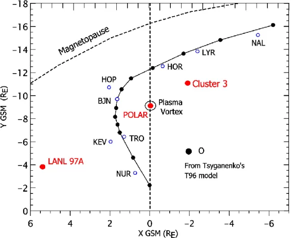
Fig. 1. The positions of the Cluster 3, POLAR and LANL 97A satellites projected over the XYGSMplane are shown, along with the eight conjugate points of the ground stations NAL, LYR, HOR, HOP, BJN, TRO, KEV and NUR over the equatorial plane (open circles). The solid circle symbols correspond to a hypothetic chain of ground stations having progressively increasing latitudes, while their longitude is 19.2◦(i.e. the BJN longitude).
magnetograms. This phenomenon, characterized by ground dispersive structures, produces waveforms out of phase, and changes the pulsation polarization sense, much like the FLR mechanism (Sarafopoulos, 2005). The event under study is associated with twin-vortex ionosphere structures and can be termed as a pseudo-FLR event. Given that many works in the past that engaged with ground Pc5 pulsations do not incorpo-rate the solar wind conditions, it is probably inevitable that many events selected as FLRs are, in fact, repetitive twin-vortex structures. Under the Sarafopoulos (2004b, 2005) per-spective the observation that all the auroral ground stations show the same frequency, which is associated with succes-sive twin-vortex current systems imposed by a magnetopause surface wave, has nothing to do with the cavity mode. The latter is the subject for this study, which further extends this author thinking. Despite the large amount of work that has been conducted in the past, the issue concerning the magne-tospheric cavity mode eigenfrequencies remains controver-sial. This work tests the cavity mode model using a case study.
2 Observations
This work deals with a case study of day 181, 2001, that incorporates measurements obtained (a) in the solar wind plasma regime (Geotail and ACE satellites), (b) at the mag-netopause surface (four Cluster satellites), (c) well-inside the magnetosphere (POLAR and LANL satellites), and (d) on the Earth’s surface (through the IMAGE array stations corre-sponding to the dawn sector plasma sheet). As a result, first, we have knowledge of the exo-magnetosphere conditions de-termining the energy input for the system. Second, we are certain that the magnetopause surface actually oscillates and propagates inward compressional waves which are associ-ated with significant power spectral density (PSD). Third, the in-situ measurements within the magnetosphere give us the opportunity to probe the local FLRs, or the supposed cav-ity/waveguide mode oscillations. Finally, the ground magne-tograms are of crucial importance to trace the ionosphere re-sponse and classify the ground signatures according to their spatial and temporal structures. The same time interval was studied, in part, by Sarafopoulos (2004b); and Fig. 1 presents the result from the mapping process of the IMAGE array ground stations (i.e. NAL, LYR, HOR, HOP, BJN, TRO,
KEV and NUR) via Tsyganenko’s T96 model (Tsyganenko, 1995, 1996) over the equatorial plane, something which is shown previously by Sarafopoulos (2004b, in his Fig. 10). The open circle symbols correspond to the real ground sta-tion coordinates, whereas the solid circles correspond to a hypothetic chain of ground stations having the same geo-graphic longitude of 19.2◦ (i.e. the BJN station longitude). Eventually, the integration of all the available information will enable us to search in depth whether a cavity/waveguide excitation mode in the Pc5 band of frequencies has actually taken place.
2.1 Response of the POLAR satellite
We examine the Pc5 frequency pulsations of plasma density and magnetic field that occur during a pass of the POLAR satellite along the dawn meridian and close to the geomag-netic equator; an interval of two hours (03:45 to 05:45 UT) of day 181, 2001, is under study. At 04:50 UT the POLAR satellite was positioned (see Fig. 1) at (X, Y, Z)GSM=(0.107,
−9.16, 2.04) RE. We use plasma data from the Thermal Ion
Dynamics Experiment (TIDE), vector magnetic field data from the Magnetic Field Experiment (MFE), and electric field (Exyand Ez)measurements from the Electric Field
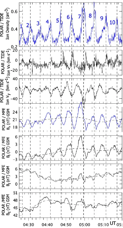
In-strument (EFI). Figure 2 clearly shows 10 variation cycles (pulsations) observed by POLAR from 04:25 to 05:20 UT. The periodicity T is exactly 6 min around the time of the largest amplitude waves. The plasma ion density (top panel) and velocity Vxand Vy components (second and third
pan-els, respectively) are very well modulated by the wave. The strongest component of the magnetic field oscillation is the Bx(fourth panel), while the Byand Bzcomponents are weak
and somewhat irregular (not shown here). Instead of pre-senting Byand Bz, we prefer to show the compressional and
transverse components of the GSM vector magnetic field that is transformed to a field-aligned coordinate system in which
ˆc is the unit vector along the average field for the interval
of Fig. 2; ˆı=ˆe x ˆc, where ˆe is the duskward unit vector, and
j=ˆc x ˆı. The new components are the transverse components
Bi and Bj, and the compressional component Bc (bottom
three panels). The Bi is almost identical to the Bx shown
in the fourth panel. In this POLAR position, along the dawn meridian, the X direction is azimuthal, while the Y direction is nearly radial. Therefore, the pulsations under study show clearly a toroidal mode of waves.
Figure 3 keeps a close watch on two variation cycles (marked as A and B along the ion density profile, top panel), which are representative of the whole event. The electric field shows a strong oscillation in the Ez component
(bot-tom panel) and a weaker one over the XY plane (fifth panel). The dominant variation for the electric field component Ez
leads the variation for the dominant magnetic field compo-nent Bx (fourth panel) by 90◦. This phase relation implies
a standing transverse wave at the fundamental mode. In particular, it shows the same frequency, at almost the same site, as in the case studied by Mitchell et al. (1990) us-ing the ISEE 1 and 2 satellites. It is worth noticus-ing that
there is a quantitative agreement between the velocities de-rived from the plasma experiment and the observed electric field: For instance, given that the Vy prevails over the Vx,
then Ex≈Exy≈VyBz≈30 km·s−1∗32 nT≈1 mV/m, which is
the directly measured value via the EFI instrument. Given that for standing Alfv´en waves the density remains constant, we conclude that the periodic density variations have to be associated with the compressional Bccomponent of the
mag-netic field (Fig. 2, bottom panel).
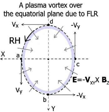
The hodogram for the velocity components Vxand Vy, as
it results from a careful inspection of the two representatively shown variation cycles in Fig. 3, is schematically drawn in Fig. 4. Each variation cycle corresponds to a plasma vor-tex with an average diameter of ∼0.5 RE. The letters marked
along the Vxand Vytraces in Fig. 3 correspond to those used
in the hodogram of Fig. 4. The polarization sense is right-handed (RH), and each vortex over the XY plane is associ-ated with a converging electric field topology marked with arrows across the circular plasma path in Fig. 4. The elec-tric field has the value E=−Uxyx Bz, and as it applies over
the ionosphere Joule dissipation takes place. If this plasma sheet vortex is projected over the ionosphere and is scaled down ∼30 times (Glassmeier et al., 1999), then it is probable that the ionosphere currents associated with this vortex will not be detectable by the ground-based magnetometers (be-cause of the spatial integration effect). In summary, Fig. 2 shows ten (out of more than twenty) successive vortex struc-tures associated with almost monochromatic oscillations of Bxwith T=6 min, which, we believe, to be the resonant
ring-ing of the medium at this L shell region. This pulsation event occurs with very low geomagnetic activity and the magne-topause surface probably constitutes the broad-band energy source for the waves under investigation.
2.2 Solar wind conditions obtained by Geotail and ACE In parallel to the repetitive plasma vortices seen by POLAR, it is of great importance to look at the solar wind conditions. Although for this event conditions are essentially analyzed in a previous work (Sarafopoulos, 2004b; Figs. 1, 4 and 5) it is useful, however, to present here the main solar wind variations that influence the magnetosphere. Additionally, we incorporate, for the first time, the most critical parameter which is the solar wind dynamic pressure. We mention that Geotail and ACE were located at (X, Y, Z)GSE=(15.27, 2.43,
1.66) and (247.8, 20.4, 14.3) RE, respectively, at 05:00 UT.
Figure 5 shows, from top to bottom: (a) the three major IMF amplitude depressions recorded by Geotail, marked with the capital letters A, B and C; (b) the solar wind ion pressure (in nPa) and density (in cm−3) measured by Geotail; (c) the ACE satellite magnetic field amplitude shifted in time 71 min to match the Geotail data, and (d) the Cluster 3 By
component of the magnetic field showing three intermittent exits of the satellite from the plasma mantle into the magne-tosheath. The negative value of Byin the magnetosheath was
inferred by the IMF measured on board Geotail (not shown here). Although the resolution time of the Geotail CPI/SWA
Fig. 2. Measurements from the POLAR satellite: (a) ten variation cycles of the ion density (in cm−3), (b) ion Vx and Vy velocities (in km s−1), (c) magnetic field Bx component (in nTs), and (d) the transverse Bi and Bj and compressional Bccomponents (bottom three panels) of the GSM vector magnetic field, which is transformed to a field-aligned coordinate system in which ˆc is the unit vector along the average field for the shown interval, ˆı=ˆe x ˆc, where ˆe is the duskward unit vector, and j=ˆc x ˆı. The toroidal character of waves is apparent.
Fig. 3. Two variation cycles of POLAR ion density (top panel) asso-ciated with the ion velocities Vxand Vy(second and third panels), the magnetic field Bxtoroidal wave (fourth panel) and the electric field Exyand Ezcomponents (in mV m−1).
plasma experiment is ∼51 s, nevertheless, we are certain that three major solar wind pressure increases are anticorrelated to the IMF amplitude depressions. Then, these pressure vari-ations are applied over the magnetosphere, forcing Cluster 3 to exit three times out of the magnetosphere cavity (bot-tom panel). Cluster 3 was located at (X, Y, Z)GSE=(−1.9,
−10.67, 8.56) RE, at 05:00 UT (Fig. 1). The dashed line in
the top panel results as a polynomial fitting of order four. The ACE magnetic field trace (fourth panel) confirms that the three characteristic variations marked as A, B and C are inherent to the solar wind plasma regime.
2.3 Response of the LANL 97A satellite
The geographic longitude for the geostationary satellite LANL 97A is 70.2◦, and at 05:00 UT it is positioned at (X, Y)=(5.42, −3.77) RE. This dayside position (Fig. 1)
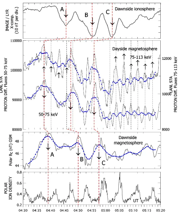
allows 97A to be affected earlier than the POLAR satel-lite from the three solar wind pressure pulses (Sarafopou-los, 2004b). Figure 6, from top to bottom, shows (a) the
Fig. 4. One plasma vortex (out of ten shown in Fig. 1) is schemati-cally shown as the hodogram of Vxand Vytaken from Fig. 3. The letters a-d show a velocity vector reorientation in steps of 90◦.
LYR station X-component magnetogram with three distinct decreases marked with the capital letters A, B and C; (b) the 97A differential fluxes for two energetic proton chan-nels with energies 50–75 and 75–113 keV (second panel, thin lines); (c) the magnetic field compressional component Bc
measured by POLAR; and (d) the POLAR ion density pro-file. The dotted curves in Fig. 6 correspond to low-pass fil-tered data with cutoff frequencies 2 and 2.4 mHz for the PO-LAR (third panel) and LANL 97A data, respectively. The applied frequency cutoffs are dictated by the power spectra, which are presented later on. These filtered energetic proton fluxes of 97A, as well as the magnetic field component Bc
of POLAR, clearly show three major increases that are obvi-ously associated with the compressions A, B and C. In this way, at the LANL 97A site, it is demonstrated that a wave with a periodicity of ∼2.5 min is superimposed over the three major decreases caused by the solar wind pressure pulses. The thin-dashed vertical lines (second panel) emphasize the high frequency wave with T=2.5 min. The three thick-dashed vertical lines mark the occurrence times of pressure pulses at different sites. Although the POLAR magnetic field pulsa-tions are largely non-compressive, with a dominant Bx
os-cillation, however, we recognize a weak compressional com-ponent with 1B/B∼=0.045, which is modulated by the three magnetosphere compressions. Much like the fact that the POLAR ion density profile shows a single unique oscilla-tion frequency, which is interpreted as the manifestaoscilla-tion of the local FLR phenomenon at L∼=9.4, the 97A energetic par-ticle discrete and stable periodicity of ∼2.5 min reflects the local FLR at L=6.6. It seems that the 97A particle fluxes re-spond passively to the magnetic field structure oscillations.
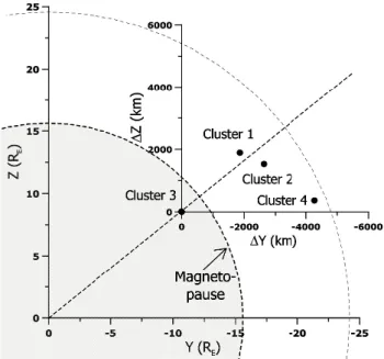
The Cluster 3 spacecraft, at 05:00 UT, was positioned at (X, Y, Z)GSE=(−1.9, −10.67, 8.56) RE, and Cluster 1, 2, and 4,
relatively to Cluster 3, were positioned at (1X1, 1Y1, 1Z1)=(323, −1918, 1907) km, (1X2, 1Y2, 1Z3)=(−1550, −2715, 1542) km, and (1X4, 1Y4, 1Z4)=(−1688, −4357, 389) km.
Cluster 3 remains at the high latitude boundary layer (HLBL) or plasma mantle, and its position (being the innermost of all the four satellites) is marked in Fig. 7 over the YZ cross-sectional plane. The other Cluster positions, relatively to Cluster 3, are shown using the axis 1Y and 1Z. The cir-cular thick-dashed line represents an ideal circir-cular magne-topause surface, and Cluster 3 is contained within this bound-ary. When each of the three solar wind pressure increases re-duces the magnetotail diameter, Cluster 3 crosses the bound-ary and exits into the magnetosheath. The latter is evi-dent from the bottom panel of Fig. 5 (see also the Fig. 5 in the work of Sarafopoulos, 2004b) showing the Cluster 3 By
magnetic field component measured by the FGM experiment (Balogh et al., 1997). The negative values along the Bytrace
represent the magnetic field lines that are draped around the magnetopause, given that the IMF has an intense negative By component about –3nT. Therefore, the three successive
exits of Cluster 3 are caused by three intense compressions applied over the magnetopause. The resulted surface wave propagates tailward with an estimated velocity ∼210 km·s−1, a surface wavelength ∼16 RE, and an azimuthal wave
num-ber m∼=6 (Sarafopoulos, 2004b).
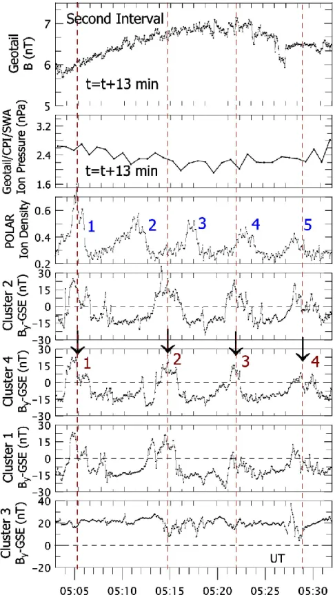
After the just presented “first time interval” the situation seems to be radically different. The amplitude of the mag-netopause surface wave is apparently significantly reduced, and consequently, Cluster 3 remains permanently inside the magnetopause. In contrast, the other three Cluster satel-lites remain essentially in the magnetosheath plasma regime (By<0) and quasi-periodically enter into the magnetosphere
(By>0). The latter is clearly demonstrated via Fig. 8,
show-ing the By responses for all the four Cluster satellites, in
four successive magnetotail expansions/contractions. This “second time interval” of Fig. 8 is not associated with an intense ULF activity visible along the IMF amplitude trace (first panel) or the solar wind ion pressure (second panel), in contrast to the situation of the preceding period of Fig. 5. Ac-tually, the Geotail time series, which are time-shifted 13 min to match the Cluster data, do not show any repetitive
varia-Fig. 5. From top to bottom: (a) the IMF amplitude (in nT) recorded by Geotail, showing three major depressions marked with the cap-ital letters A, B and C; (b) the solar wind ion pressure (in nPa) and density (in cm−3) measured by Geotail; (c) the ACE satel-lite magnetic field amplitude shifted in time 71 min to match the Geotail data, and (d) the Cluster 3 Bycomponent of the magnetic field showing three intermittent exits of the satellite from the plasma mantle into the magnetosheath.
tion which could be associated with the four variation cycles marked with the numbers 1–4 along the Cluster 4 Bytrace, or
the five variation cycles marked with the numbers 1–5 along the POLAR ion density trace (third panel). In this case, we are almost certain that the surface wave is not directly driven by the solar wind conditions, and that KHI may be the spe-cific mechanism producing it.
3 Discussion
3.1 Simultaneous pseudo- and authentic-FLRs
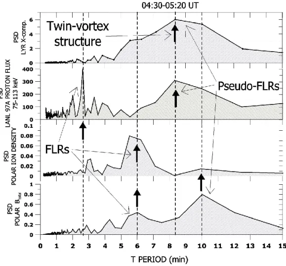
In Fig. 9 the power spectral densities (PSDs) are computed for a few time series obtained from the POLAR and LANL
Fig. 6. From top to bottom: X-component magnetogram from the ground station LYR; differential fluxes from the two energetic proton LANL 97A channels (50–75 and 75–113 keV, thin lines); and compressional magnetic field component and ion density from the POLAR satellite. The dotted-thick lines represent low-pass filtered data, while the capital letters A, B and C mark the occurrence times for the three solar wind pressure pulses, which, in turn, modulate the 97 A fluxes and the POLAR total magnetic field trace. The 97A fluxes are clearly modulated by a wave of period T∼=2.5 min.
97A satellites and the ground station LYR. The purpose is to determine the underlying excitation mechanisms for the identified periodic variations. All four spectra shown are computed for the interval 04:30–05:20 UT, corresponding exactly to that shown in Fig. 6, and having the prominent fea-ture that three successive exo-magnetosphere compressions occur within it. The X-component magnetogram from the LYR station (first panel) shows wave activity confined
be-tween T=5.5 and 12 min; with the assumption that signif-icant frequencies are those lying above the half-maximum PSD level. At this moment we mention, again, that the X component magnetograms of all the IMAGE stations demon-strate, for the case under study, the latitude dependent dis-persive structures shown by Sarafopoulos (2004b, Fig. 1) and are interpreted as the manifestation of pseudo-FLRs, which are associated with the formation of twin-vortex
The ion density PSD of POLAR (Fig. 9, third panel) shows a unique dominant periodicity at T=6 min originated by the local FLR mechanism. Finally, the PSD computed from the POLAR magnetic field strength (fourth panel) shows two pe-riodicities: one at T=6 min, which is the already identified lo-cal FLR oscillation, and a second at T∼=10 min, which is most probably caused by the solar wind pressure variation. There-fore, we believe that the differentiation between authentic-and pseudo-FLRs is very clear. It is demonstrated, with in-situ measurements, that genuine FLRs are actually excited as monochromatic waves at two widely separated sites within the magnetospheric cavity. In contrast, the pseudo-FLRs de-tected by ground magnetometers or satellites (and marked in Fig. 9) are more broad-band in their character and probably are driven by the three exo-magnetosphere successive com-pressions.
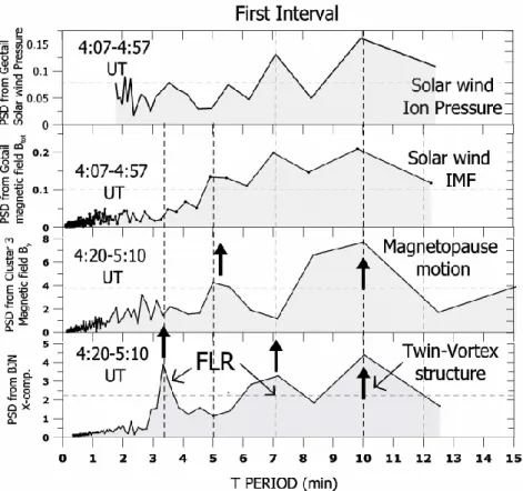
3.2 Energy source for the FLR and non-FLR oscillations To understand better the interaction among the solar wind variations, the magnetopause motion and the ionosphere cur-rents, we compute a few more power spectra. We divide the whole interval under study into two subintervals: the first one that essentially corresponds to the occurrence time of the three solar wind pulses (Fig. 10, interval from 04:20 to 05:10 UT, in which the Geotail data are time-shifted 13 min to match the magnetosphere data), and the second one, in which, although the magnetopause surface quasi-periodically oscillates as well (Fig. 11, interval from 05:03 to 05:32 UT, that is exactly that presented in Fig. 8), the solar wind parameters do not show any significant variation. First, we compute for both intervals the PSDs of the IMF ampli-tude (Fig. 10, second panel and Fig. 11, top panel), given that these high resolution measurements are anticorrelated to the solar wind pressure (Fig. 5). Actually, the computed PSD for the solar wind ion pressure (Fig. 10, first panel) shows the same two major peaks as the IMF, even though the plasma data are of low resolution. The result is that (a) the input energy of the solar wind has actually a broad-band charac-ter (T=5–12 min), and (b) the input energy is much smaller for the second interval, given that both of the computed IMF PSDs are displayed in scale. The high latitude ground station LYR (Fig. 9) has essentially a similar power spectrum as the IMF amplitude in Fig. 10. During both subintervals the
mag-Fig. 7. The Cluster 3 position projected over the YZ plane, and the Cluster 1, 2 and 4 positions as pairs of (1Y, 1Z) in refer-ence to Cluster 3 are shown. The ideally circular magnetopause surface is drawn with thick-dashed line and encloses the Cluster 3 site throughout the studied event, except for the short intervals that coincide with the occurrence times of the three solar wind pressure pulses.
netopause surface oscillates, while the magnetic field compo-nent By of Cluster 3 (first subinterval; Fig. 5) and Cluster 2
(second subinterval; Fig. 8) is directly associated with the spacecraft’ entries into, and exits out of, the magnetosphere. In both subintervals the magnetopause oscillates and actually constitutes a broad-band energy source that is able to propa-gate inward fast mode waves.
The Cluster 2 By line at T∼=3.5 min (Fig. 11) may excite
the FLR, which is also visible along the trace of the BJN PSD (Fig. 11, bottom panel). The same line of T∼=3.5 min, for the BJN station, is strong during the first subinterval (Fig. 10, fourth panel) as well, in which a second line with T∼=7 min (Fig. 10) is simultaneously apparent. The conjugate point for the BJN station over the XY plane, as it is determined using the T96 model, is (X, Y)=(1.64, −9.7) RE. This point
corresponds to L=9.84, and given that the POLAR at L=9.4 is associated with the FLR period of 6 min, then it is plausible to hypothesize that the BJN line of T∼=7 min is probably the local resonant frequency that corresponds to the fundamental mode oscillation, while the line at ∼3.5 min corresponds to the first harmonic.
3.3 The cavity/waveguide mode is not revealed
The discrete and stable frequencies with T∼=2.5 and 6 min, which are locally observed by LANL 97A and POLAR, re-spectively, as well as the periods of T=3.5 and 7 min de-tected by the BJN ground station, are probably produced by spatially restricted FLRs, and consequently, they are not the
Fig. 8. From top to bottom: Geotail magnetic field amplitude and solar wind ion pressure shifted in time 13 min to match the POLAR and Cluster data; POLAR ion density profile, and the Bycomponent of the magnetic field for each of the four Cluster satellites. During this interval Cluster 3 remains inside the magnetopause (By>0), whereas the other three Cluster satellites remain in magnetosheath (By<0) and enter into the magnetosphere proper only for four short intervals. For the same interval the POLAR ion density shows five complete variation cycles.
Fig. 9. Power spectral densities (PSDs) of the interval 04:30-05:20 UT for (a) the X-component magnetogram of LYR, (b) the 75–113 keV proton differential fluxes of LANL 97A, (c) the POLAR ion density, and (d) the POLAR magnetic field magnitude. The almost monochro-matic lines of T=2.5 and 6 min correspond to FLRs, whereas the broad-band response of LYR is associated with the detected twin vortex ionosphere structures, which are produced by the solar wind pressure pulses.
eigenfrequencies developed within the magnetosphere from a supposed cavity/waveguide mode. The latter is obvious because if we had adopted the cavity mode scenario, then the lines of T=2.5 and 6 min should have been observed by both satellites (i.e. POLAR and 97A). Conversely, they are developed and observed locally. During the interval pre-sented in Fig. 6, 04:30–05:20 UT, the LYR station shows a main frequency at T∼=8.5 min (Fig. 9), however, the wave activity has a more broad-band character that extends from T∼=5.5 to 12 min. Therefore, by itself, the ground response is not monochromatic, as the cavity mode model requires. We mention, again, that the cavity mode model was introduced to reconcile the development of monochromatic pulsations ob-served on the ground with a broad-band energy input via the KHI. The PSD of LYR (Fig. 9) probably reflects the broad-band character seen in the solar wind variation parameters that directly affect the magnetosphere. Actually, apart from the unambiguously recognized FLR frequencies, the POLAR and 97A measurements show a wave activity that is due to the solar wind conditions rather than to the cavity mode. As
a matter of fact, only the time series dependent on the to-tal magnetic field B are affected within the magnetosphere. The whole magnetosphere is successively compressed and decompressed, the magnetic field amplitude is directly af-fected (the POLAR case, Fig. 6) and, in turn, the energetic particle fluxes at the 97A site are appropriately modulated. The POLAR ion density remains intact by the magnetic field magnitude microvariations, while the plasma vortices are es-sentially associated with the toroidal magnetic field oscilla-tions.
The magnetopause surface constitutes a rather broad-band source of waves. The Bytrace of Cluster provides the
appro-priate parameter associated with the motion of the magne-topause boundary and its structure; and the ByPSD may
cor-respond to the imparted energy across the boundary. There-fore, the periods included in the band T=8–11 min (Figs. 10 and 11, for the Cluster By PSDs) probably force the
mag-netosphere to oscillate, whereas a cavity/waveguide mode is not developed. Under this perspective, the LYR and BJN sta-tion responses, with maximum PSDs at T∼=8.3 and 10 min,
Fig. 10. For the “first interval” 04:20–05:10 UT the PSDs are computed for (a) the Geotail solar wind ion pressure, (b) the Geotail magnetic field amplitude upstream of the bow shock, (b) the Cluster 3 Bymagnetic field component, and (c) the X-component magnetogram from the BJN station. The Geotail data are shifted 13 min to match the Cluster measurements. The BJN station shows one peak PSD corresponding to the twin vortex structures (like the other ground stations), however, two distinct resonant frequencies with T=3.5 and 7 min are also evident.
Fig. 11. For the “second interval” 05:03–05:32 UT the PSDs are presented with the same format as in Fig. 10. The BJN station shows the resonant frequency of T=3.5 min, too.
within the magnetosphere cavity. However, we fail to recog-nize any element that might support the cavity mode model. 3.4 The cavity mode model of Samson
The cavity mode model of Samson (CMS) is associated with the discrete (monochromatic) lines at T=4, 4.9, 6.4, 8.8 and 12.8 min. Our intention is to scrutinize each line in the light of the presented case study, and in particular, to study the first subinterval which is directly associated with the three in-tense solar wind pressure pulses. Apparently, the CMS lines of 4, 4.9, and 12.8 min are not observed, neither by satel-lite nor by ground stations. The CMS line of 6.4 min may agree with the POLAR magnetic field and ion density oscil-lation frequency, but the LANL 97A satellite, at the same time, does not trace such a line. The CMS line of 8.8 min is not observed in the POLAR magnetic field and the BJN X-component spectra, which show a peak PSD of T=10 min. Most importantly, the line of 8.8 min is within the frequency band extended from 8 to 10 min, corresponding to the forma-tion of the twin vortex structures, the so-called pseudo-FLRs (Sarafopoulos, 2005). The latter are associated with the dis-persive structures of ground magnetograms shown, for the case under study, by Sarafopoulos (2004b, Fig. 1). Actually, the LYR station PSD is peaked in between T=8 and 10 min (Fig. 9, top panel); and the same result is inferred from the Cluster 3 By PSD (Fig. 10, third panel), which reflects the
magnetopause dynamics. Therefore, our crucial conclusion is that no CMS frequency is detected in this case study.
4 Conclusion
Despite the well-organized multipoint observations, no evi-dence of any eigenfrequency associated with a cavity mode oscillation is detected within the magnetosphere. Our final opinion is that we have to look at a few more similar case studies with multipoint observations. If the additional obser-vational evidence aligns with this study result, then we will have to abandon the idea that the magnetosphere resonates as a cavity within the Pc5 frequency band.
Acknowledgements. We are grateful to all Principal Investigators
of the experiments MGF and CPI/SWA of Geotail; TIDE, MFE and EFI of POLAR; MAG and SWEPAM of ACE; FGM of Cluster and
Planet. Space Sci., 34, 371–385, 1986.
Anderson, B. J., Engebretson, M. J., Rounds, S. P., Zanetti, L. J., and Potemra, T. A.: A statistical study of Pc 3-5 pulsations observed by the AMPTE/CCE magnetic fields experiment, 1, Occurrence distributions, J. Geophys. Res., 95, 10 495–10 523, 1990.
Baker, Gregory J., Donovan, E. F., and Jackel, Brian J.: A compre-hensive survey of auroral latitude Pc5 pulsation characteristics, J. Geophys. Res, 108A10, 1384, doi:10.1029/2002JA009801, 2003.
Balogh, A., Dunlop, M. W., Cowley, S. W. H., Southwood, D. J., and Thomlinson, J. G., and the Cluster magnetometer team: The Cluster Magnetic Field Investigation, Space Sci. Rev., 79, 65–92, 1997.
Chen, L. and Hasegawa, A.: A theory of longperiod magnetic pul-sations 1. Steady state excitation of field line resonance, J. Geo-phys. Res., 79, 1024–1032, 1974.
Chisham, G. and Orr, D.: A statistical study of the local time asym-metry of Pc5 ULF wave characteristics observed at midlatitudes by SAMNET, J. Geophys. Res., 102(A11), 24 339–24 350, 1997. Engebretson, M. J., Zanetti, L. J., Potemra, T. A., and Acuna, M. H.: Harmonically structured ULF pulsations observed by the AMPTE CCE magnetic field experiment, Geophys. Res. Lett., 13, 905–908, 1986.
Fenrich, F. R., Samson, J. C., Softko, G., and Greenwald, R. A.: ULF high- and low- m field line resonances observed with the Super Dual Auroral Radar Network, J. Geophys. Res., 100(A11), 21 535–21 547, 1995.
Francia, P. and Villante, U.: Some evidence of ground power en-hancements at frequencies of global magnetospheric modes at low latitudes, Ann. Geophys., 15, 17–23, 1997,
SRef-ID: 1432-0576/ag/1997-15-17.
Harrold, B. G. and Samson, J. C.: Standing ULF modes of the mag-netosphere: a theory, Geophys. Res. Lett., 19, 1811–1814, 1992. Hughes, W. J.: Magnetospheric ULF waves: A tutorial with a his-torical perspective, in Solar Wind Sources of Magnetospheric ULF Waves, Geophysical Monogr. Ser., vol. 81, (Eds.) Engebret-son, M. J., Takahashi, K., and Scholer, M., 1–11, AGU, Wash-ington, D.C., 1994.
Glassmeier, K. H.: ULF pulsations, in Handbook of Atmospheric Electrodynamics, Volume II, (Ed.) Volland, H., 463–502, Uni-versity of Bonn, Germany, 1995a.
Glassmeier, K. H.: Ultralow-frequency pulsations: Earth and Jupiter compared, Adv. Space Res., 16, 4, 4209–4218, 1995b. Glassmeier, K. H., Othmer, C., Cramm, R., Stellmacher, M., and
Engebretson, M.: Magnetospheric field line resonances: A com-parative planetology approach, Surveys in Geophys. 20, 61–109, 1999.
Kivelson, M. G., Etcheto, J., and Trotignon, J. G.: Global compres-sional oscillations of the terrestrial magnetosphere: the evidence and a model, J. Geophys. Res., 89, 9851–9856, 1984.
Kivelson, M. G. and Southwood, D. J.: Resonant ULF waves: A new interpretation, Geophys. Res. Lett., 12, 49–52, 1985. Kivelson, M. G. and Southwood, D. J.: Coupling of global
magne-tospheric MHD eigenmodes to field line resonances, J. Geophys. Res., 91, 4345–4351, 1986.
Korotova, G. I. and Sibeck, D. G.: A case study of transient event motion in the magnetosphere and in the ionosphere, J. Geophys. Res., 100, 35–46, 1995.
Lee, D.-H. and Lysak, R. L.: Impulsive excitation of ULF waves in the three-dimensional dipole model: the initial results, J. Geo-phys. Res., 96, 3479–3486, 1991a.
Lee, D.-H. and Lysak, R. L.: Monochromatic ULF wave excitation in the dipole magnetosphere, J. Geophys. Res., 96, 5811–5817, 1991b.
Lee, D.-H. and Lysak, R. L.: Magnetospheric ULF wave coupling in the dipole field: the impulsive excitation, J. Geophys. Res., 94, 17 097–17 103, 1989.
Mathie R. A., Mann I. R., Menk F. W., and Orr D.: Pc5 ULF pul-sations associated with waveguide modes observed with the IM-AGE magnetometer array, J. Geophys. Res., 104, 7025–7036, 1999.
Matsuoka, H., Takahashi, K., Yumoto, K., Anderson, B. J., and Sibeck, D. G.: Observation and modeling of compressional Pi 3 magnetic pulsations, J. Geophys. Res., 100, 12 103–12 115, 1995.
McDiarmid, D. R. and Allan, W.: Simulation and analysis of auroral radar signatures generated by a magnetospheric cavity mode, J. Geophys. Res., 95(A12), 20 911–20 922, 1990.
Mitchell, D. G., Engebretson, M. J., Williams, D. J., Cattell, C. A., and Lundin, R.: Pc5 Pulsations in the outer dawn magnetosphere seen by ISEE 1 and 2, J. Geophys. Res., 95, 967–975, 1990. Nos´e, M., Iyemori, T., Sugiura, M., and Slavin, J. A.: A strong
dawn/dusk asymmetry in Pc 5 pulsation occurrence observed by the DE-1 satellite, Geophys. Res. Lett., 22, 2053–2056, 1995. Provan, G. and Yeoman, T. K.: A comparison of field-line
reso-nances observed at the Goose Bay and Wick radars, Ann. Geo-phys., 15, 231–235, 1997,
SRef-ID: 1432-0576/ag/1997-15-231.
Samson, J. C., Harrold, B. G., Ruohoniem, J. M., Greenwald, R. A., and Walker, A. D. M.: Field line resonances associated with MHD waveguides in the magnetosphere, Geophys. Res. Lett., 19, 441–444, 1992.
Samson, J. C., Greenwald, R. A., Ruohoniemi, J. M., Hughes, T. J., and Wallis, D. D.: Magnetometer and radar observations of mag-netohydrodynamic cavity modes in the earth’s magnetosphere, Can. J. Phys., 69, 929–937, 1991.
Sarafopoulos, D. V.: Long duration Pc 5 compressional pulsations inside the Earth’s magnetotail lobes, Ann. Geophys., 13, 926– 937, 1995,
SRef-ID: 1432-0576/ag/1995-13-926.
Sarafopoulos, D. V.: Distinct solar wind pressure pulses produc-ing convection twin-vortex systems in the ionosphere, Ann. Geo-phys., 22, 2201–2211, 2004a,
SRef-ID: 1432-0576/ag/2004-22-2201.
Sarafopoulos, D. V.: Repetitive X-line Hall current structures over the dawnside ionosphere induced by successive exo-magnetosphere pressure pulses, Ann. Geophys., 22, 4153–4163, 2004b,
SRef-ID: 1432-0576/ag/2004-22-4153.
Sarafopoulos, D. V.: Pseudo-Field Line Resonances in ground Pc5 pulsation events, Ann. Geophys., 23, 593–608, 2005,
SRef-ID: 1432-0576/ag/2005-23-593.
Shimazu, H., Araki, T., Kamei, T., and Hanado, H.: A symmetric appearance of Pc 5 on dawn and dusk side associated with solar wind dynamic pressure enhancement, J. Geomag. Geoelectr., 47, 177–189, 1995.
Southwood, D. J.: Some features of field line resonances in the magnetosphere, Planet. Space Sci., 22, 483–491, 1974.
Takahashi, K.: ULF waves: 1997 IAGA division 3 reporter review, Ann. Geophys., 16, 787–803, 1998,
SRef-ID: 1432-0576/ag/1998-16-787.
Tsyganenko, N. A.: Modelling the Earth’s magnetospheric mag-netic field confined within a realistic magnetopause, J. Geophys. Res., 100, 5599–5612, 1995.
Tsyganenko, N. A.: Effects of the solar wind conditions on the global magnetospheric configuration as deduced from data-based field models, European Space Agency Spec. Publ., ESA SP-389, 181, 1996.
Walker, A. D. M., Ruohouniemi, J. M., Baker, K. B., Greenwald, R. A., and Samson, J. C.: Spatial and temporal behaviour of ULF pulsations observed by the Goose Bay HF radar, J. Geo-phys. Res., 97, 12 187–12 202, 1992.
Ziesolleck, C. W. S. and McDiarmid, D. R.: Statistical survey of auroral latitude Pc 5 spectral and polarization characteristics, J. Geophys. Res., 100, 19 299–19 312, 1995.