HAL Id: hal-00327752
https://hal.archives-ouvertes.fr/hal-00327752
Submitted on 12 Jan 2016
HAL is a multi-disciplinary open access
archive for the deposit and dissemination of
sci-entific research documents, whether they are
pub-lished or not. The documents may come from
teaching and research institutions in France or
abroad, or from public or private research centers.
L’archive ouverte pluridisciplinaire HAL, est
destinée au dépôt et à la diffusion de documents
scientifiques de niveau recherche, publiés ou non,
émanant des établissements d’enseignement et de
recherche français ou étrangers, des laboratoires
publics ou privés.
Chemistry Experiment (ACE)
T. Kerzenmacher, M.A. Wolff, K. Strong, E. Dupuy, K.A. Walker, L.K.
Amekudzi, R.L. Batchelor, P.F. Bernath, Gwenaël Berthet, T. Blumenstock,
et al.
To cite this version:
T. Kerzenmacher, M.A. Wolff, K. Strong, E. Dupuy, K.A. Walker, et al.. Validation of NO2 and NO
from the Atmospheric Chemistry Experiment (ACE). Atmospheric Chemistry and Physics, European
Geosciences Union, 2008, 8 (19), pp.5801-5841. �10.5194/acp-8-5801-2008�. �hal-00327752�
www.atmos-chem-phys.net/8/5801/2008/ © Author(s) 2008. This work is distributed under the Creative Commons Attribution 3.0 License.
Chemistry
and Physics
Validation of NO
2
and NO from the Atmospheric Chemistry
Experiment (ACE)
T. Kerzenmacher1, M. A. Wolff1, K. Strong1, E. Dupuy2, K. A. Walker1,2, L. K. Amekudzi3, R. L. Batchelor1,
P. F. Bernath4,2, G. Berthet5, T. Blumenstock6, C. D. Boone2, K. Bramstedt3, C. Brogniez7, S. Brohede8,
J. P. Burrows3, V. Catoire5, J. Dodion9, J. R. Drummond10,1, D. G. Dufour11, B. Funke12, D. Fussen9, F. Goutail13,
D. W. T. Griffith14, C. S. Haley15, F. Hendrick9, M. H¨opfner6, N. Huret5, N. Jones14, J. Kar1, I. Kramer6,
E. J. Llewellyn16, M. L´opez-Puertas12, G. Manney17,18, C. T. McElroy19,1, C. A. McLinden19, S. Melo20, S. Mikuteit6,
D. Murtagh8, F. Nichitiu1, J. Notholt3, C. Nowlan1, C. Piccolo21, J.-P. Pommereau13, C. Randall22, P. Raspollini23,
M. Ridolfi24, A. Richter3, M. Schneider6, O. Schrems25, M. Silicani20, G. P. Stiller6, J. Taylor1, C. T´etard7,
M. Toohey1, F. Vanhellemont9, T. Warneke3, J. M. Zawodny26, and J. Zou1
1Department of Physics, University of Toronto, Toronto, Ontario, Canada
2Department of Chemistry, University of Waterloo, Waterloo, Ontario, Canada
3Institute of Environmental Physics, Institute of Remote Sensing, Universit¨at Bremen, Bremen, Germany
4Department of Chemistry, University of York, Heslington, York, UK
5Laboratoire de Physique et Chimie de l’Environnement, CNRS–Universit´e d’Orl´eans, Orl´eans, France
6Forschungszentrum Karlsruhe und Universit¨at Karlsruhe, Inst. f¨ur Meteorologie und Klimaforschung (IMK), Karlsruhe,
Germany
7Laboratoire d’Optique Atmosph´erique, Universit´e des sciences et technologies de Lille, Villeneuve d’Ascq, France
8Department of Radio and Space Science, Chalmers University of Technology, G¨oteborg, Sweden
9Belgisch Instituut voor Ruimte-A¨eronomie–Institut d’A´eronomie Spatiale de Belgique (IASB-BIRA), Bruxelles, Belgium
10Department of Physics & Atmospheric Science, Dalhousie University, Halifax, Nova Scotia, Canada
11Picomole Instruments Inc., Edmonton, Alberta, Canada
12Instituto de Astrof´ısica de Andaluc´ıa, CSIC, Granada, Spain
13Service d’A´eronomie–CNRS, Verri`eres-le-Buisson, France
14School of Chemistry, University of Wollongong, Wollongong, Australia
15Centre for Research in Earth and Space Science, York University, Toronto, Ontario, Canada
16Institute of Space and Atmospheric Studies, University of Saskatchewan, Saskatoon, Saskatchewan, Canada
17Jet Propulsion Laboratory, California Institute of Technology, Pasadena, CA, USA
18New Mexico Institute of Mining and Technology, Socorro, NM, USA
19Environment Canada, Downsview, Ontario, Canada
20Canadian Space Agency, St Hubert, Quebec, Canada
21Atmospheric, Oceanic and Planetary Physics, University of Oxford, Oxford, UK
22Laboratory for Atmospheric and Space Physics & Department of Atmospheric and Oceanic Sciences, University of
Colorado, Boulder, CO, USA
23Istituto di Fisica Applicata “Nello Carrara” (IFAC) del Consiglio Nazionale delle Ricerche (CNR), Firenze, Italy
24Dipartimento di Chimica Fisica e Inorganica, Universit´a di Bologna, Bologna, Italy
25Alfred Wegener Institute for Polar and Marine Research, Bremerhaven, Germany
26NASA Langley Research Center, Hampton, VA, USA
Received: 4 December 2007 – Published in Atmos. Chem. Phys. Discuss.: 14 February 2008 Revised: 14 July 2008 – Accepted: 9 August 2008 – Published: 8 October 2008
Correspondence to: T. Kerzenmacher
Abstract. Vertical profiles of NO2 and NO have been
obtained from solar occultation measurements by the At-mospheric Chemistry Experiment (ACE), using an in-frared Fourier Transform Spectrometer (ACE-FTS) and
(for NO2) an ultraviolet-visible-near-infrared spectrometer,
MAESTRO (Measurement of Aerosol Extinction in the Stratosphere and Troposphere Retrieved by Occultation). In this paper, the quality of the ACE-FTS version 2.2
NO2 and NO and the MAESTRO version 1.2 NO2 data
are assessed using other solar occultation measurements (HALOE, SAGE II, SAGE III, POAM III, SCIAMACHY), stellar occultation measurements (GOMOS), limb mea-surements (MIPAS, OSIRIS), nadir meamea-surements (SCIA-MACHY), balloon-borne measurements (SPIRALE, SAOZ) and ground-based measurements (UV-VIS, FTIR). Time dif-ferences between the comparison measurements were re-duced using either a tight coincidence criterion, or where
possible, chemical box models. ACE-FTS NO2and NO and
the MAESTRO NO2 are generally consistent with the
cor-relative data. The ACE-FTS and MAESTRO NO2 volume
mixing ratio (VMR) profiles agree with the profiles from other satellite data sets to within about 20% between 25 and 40 km, with the exception of MIPAS ESA (for ACE-FTS) and SAGE II (for ACE-FTS (sunrise) and MAESTRO) and suggest a negative bias between 23 and 40 km of about 10%. MAESTRO reports larger VMR values than the ACE-FTS. In comparisons with HALOE, ACE-FTS NO VMRs typi-cally (on average) agree to ±8% from 22 to 64 km and to +10% from 93 to 105 km, with maxima of 21% and 36%,
respectively. Partial column comparisons for NO2show that
there is quite good agreement between the ACE instruments and the FTIRs, with a mean difference of +7.3% for ACE-FTS and +12.8% for MAESTRO.
1 Introduction
This is one of two papers describing the validation of NOy
species measured by the Atmospheric Chemistry Experiment (ACE) through comparisons with coincident measurements.
The total reactive nitrogen, or NOy, family consists of
ac-tive nitrogen, NOx (NO+NO2), and all oxidized nitrogen
species, including NO3, HNO3, HNO4, ClONO2, BrONO2
and N2O5. The ACE-Fourier Transform Spectrometer
(ACE-FTS) measures all of these species, with the exception of
NO3 and BrONO2, while the Measurement of Aerosol
Ex-tinction in the Stratosphere and Troposphere Retrieved by Occultation (ACE-MAESTRO, referred to as MAESTRO in
this paper) measures NO2. The species NO2 and NO are
two of the 14 primary target species for the ACE mission. In this study, the quality of ACE-FTS version 2.2 nitrogen
diox-ide (NO2) and nitric oxide (NO) and MAESTRO version 1.2
NO2 are assessed prior to their public release. A
compan-ion paper by Wolff et al. (2008) provides an assessment of
the ACE-FTS version 2.2 nitric acid (HNO3), chlorine
ni-trate (ClONO2) and updated version 2.2 dinitrogen pentoxide
(N2O5). Validation of ACE-FTS version 2.2 measurements
of nitrous oxide (N2O), the source gas for NOy, is discussed
by Strong et al. (2008).
NO2and NO are rapidly interconverted and closely linked
through photochemical reactions in the atmosphere. As NOx,
they have a maximum lifetime of 10 to 50 h in the strato-sphere between 20 and 50 km under midlatitude equinox
con-ditions (Dessler, 2000). The NOxgas phase catalytic cycle
destroys odd oxygen in the stratosphere, while NO2and NO
also have important roles determining the polar ozone bud-get.
Remote sensing measurements of NO2and NO have been
performed since the early 1970s (e.g. Murcray et al., 1968; Ackermann and Muller, 1972; Brewer et al., 1973; Burkhardt et al., 1975; Fontanella et al., 1975; Noxon, 1975). Satel-lite instruments have been regularly measuring these species since the launch of Nimbus-7 in 1979, which carried the Stratospheric and Mesospheric Sounder (SAMS) for NO (Drummond et al., 1980) and the Limb Infrared Monitor
of the Stratosphere (LIMS) for NO and NO2 (Gille et al.,
1980). There was a visible light spectrometer on board the Solar Mesosphere Explorer (SME) spacecraft, which also
made early measurements of NO and NO2 (Mount et al.,
1984). The launch of the Upper Atmosphere Research Satel-lite (UARS) in 1991 provided measurements from the Im-proved Stratospheric and Mesospheric Sounder (ISAMS) (Taylor et al., 1993), the Cryogenic Limb Array Etalon Spec-trometer (CLAES) (Roche et al., 1993) and the HALogen Occultation Experiment (HALOE) (Russell et al., 1993).
The ACE mission builds on the heritage of a number of previous solar occultation missions, including the At-mospheric Trace MOlecule Spectroscopy (ATMOS) instru-ment (Abrams et al., 1996; Gunson et al., 1996; Newchurch et al., 1996; Manney et al., 1999), which flew on four Space Shuttle flights between 1985 and 1994. The three Stratospheric Aerosol and Gas Experiment instruments, SAGE I (McCormick et al., 1979; Chu and McCormick, 1979, 1986), SAGE II (Mauldin et al., 1985) and SAGE III (SAGE ATBD Team, 2002) all used ultraviolet-visible
(UV-VIS) solar occultation to measure NO2, as did the second
Polar Ozone and Aerosol Measurement (POAM II) (Glac-cum et al., 1996) and POAM III (Lucke et al., 1999; Ran-dall et al., 2002). The Improved Limb Atmospheric Spec-trometers (ILAS) I and II were infrared solar occultation
in-struments that also measured NO2(e.g. Sasano et al., 1999;
Nakajima et al., 2006; Irie et al., 2002; Wetzel et al., 2006). In addition to the ACE instruments, there are currently two
instruments in orbit measuring NO2 using the occultation
technique: SCIAMACHY (SCanning Imaging Absorption spectroMeter for Atmospheric CHartographY), doing solar occultation measurements, (which is its secondary measure-ment mode) (Bovensmann et al., 1999) and the stellar oc-cultation instrument GOMOS (Global Ozone Monitoring by
the Occultation of Stars) (Kyr¨ol¨a et al., 2004, and references therein).
Space-based measurements of NO2 are also being made
using several other techniques. The Global Ozone Mon-itoring Experiment GOME (Burrows et al., 1999), SCIA-MACHY (Bovensmann et al., 1999), GOME-2 (Callies et al., 2004), and the Ozone Monitoring Instrument (OMI)
(Lev-elt et al., 2006) all retrieve NO2 total columns from
nadir-viewing observations at visible wavelengths. Also using
this spectral range for NO2, but in limb-scattering mode,
is the Optical Spectrograph and Infra-Red Imager System, or OSIRIS, (Llewellyn et al., 2004) and SCIAMACHY (Bovensmann et al., 1999) in limb mode. The Michelson Interferometer for Passive Atmospheric Sounding (MIPAS)
detects both NOxspecies and is the only instrument besides
ACE-FTS that is currently measuring stratospheric NO from orbit (Fischer and Oelhaf, 1996; Fischer et al., 2008). Recent
validation studies of NO2have been performed by Brohede
et al. (2007a) for OSIRIS and Wetzel et al. (2007) for MIPAS Environmental Satellite (Envisat) operational data; the latter included a comparison with the ACE-FTS v2.2 data. In
addi-tion, measurements of NO2by GOMOS, MIPAS and
SCIA-MACHY, all on Envisat, were compared by Bracher et al. (2005a).
In this paper, we assess the quality of the ACE-FTS
ver-sion 2.2 NO2and NO data and the MAESTRO version 1.2
NO2 data through comparisons with available coincident
measurements. The paper is organized as follows. In Sect. 2, the ACE mission and the retrievals of these two species by ACE-FTS and MAESTRO are presented. Section 3 describes all of the satellite, balloon-borne and ground-based instru-ments used in this study. The validation methodology and the use of a chemical box model to account for the diurnal
vari-ability of NO2and NO are discussed in Sect. 4. In Sect. 5,
the results of vertical profile and partial column comparisons
for NO2are given, while Sect. 6 focuses on the results of the
NO and NOxcomparisons. Finally, the results are
summa-rized and conclusions regarding the quality of the ACE NO2
and NO data are provided in Sect. 7.
2 The Atmospheric Chemistry Experiment
The ACE satellite mission, in orbit since 12 August 2003, carries two instruments, the ACE-FTS (Bernath et al., 2005) and a dual spectrometer, MAESTRO (McElroy et al., 2007). Both instruments record solar occultation spectra, ACE-FTS in the infrared and MAESTRO in the UV-VIS-near-infrared, from which vertical profiles of atmospheric trace gases, tem-perature and aerosol extinction are retrieved. The SCISAT spacecraft is in a circular orbit at an altitude of 650 km, with
a 74◦ inclination angle (Bernath et al., 2005), providing up
to 15 sunrise and 15 sunset solar occultations per day. The choice of orbital parameters results in coverage of the trop-ics, midlatitudes and polar regions with an annually
repeat--90 -60 -30 0 30 60 90 Latitude 0 2 4 6 8 10 12 Frequency in %
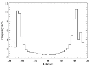
Fig. 1. Sampling frequency of 11,111 ACE satellite measurements
(February 2004 to December 2007) using 5◦latitude bins.
ing pattern, and a sampling frequency that is greatest over the Arctic and Antarctic (see Fig. 1). The primary scientific ob-jective of the ACE mission is to understand the chemical and dynamical processes that control the distribution of ozone in the stratosphere and upper troposphere, particularly in the Arctic (Bernath et al., 2005; Bernath, 2006, and references therein).
In previous studies McHugh et al. (2005) compared
ACE-FTS v1.0 NO2 to HALOE v19 NO2and found a low bias
of 0 to 10% from 22 to 35 km, and a high bias of 0 to 50% below 22 km. Comparisons between HALOE v19 and ACE-FTS v1.0 NO data were described by McHugh et al. (2005), who found that ACE-FTS NO was 10 to 20% smaller than HALOE from 25 to 55 km. Large uncertainties were present from 65 to 90 km, and ACE-FTS NO was approxi-mately 50% smaller than HALOE above 90 km. ACE-FTS
and MAESTRO NO2profiles have been compared with data
from POAM III and SAGE III (Kar et al., 2007) and partial columns have been compared with those retrieved using the Portable Atmospheric Research Interferometric Spectrome-ter for the InfraRed (PARIS-IR), a ground-based adaptation of ACE-FTS and other ground-based spectrometers during the spring 2004 to 2006 Canadian Arctic ACE validation campaigns (Kerzenmacher et al., 2005; Fraser et al., 2008;
Sung et al., 20081; Fu et al., 2008). ACE-FTS NOxprofiles
have been used in high energy particle precipitation studies (Rinsland et al., 2005; Randall et al., 2007).
1Sung, K., Strong, K., Mittermeier, R. L., Walker K. A., Fu, D., Kerzenmacher, T., Fast, H., Bernath, P., F., Boone, C. D., Daffer, W. H., Drummond, J. R., Kolonjari, F., Loewen, P., MacQuarrie, K., and Manney, G. L.: Ground-based column measurements at Eureka, Nunavut, made using two Fourier transform infrared spectrometers in spring 2004 and 2005, and comparison with the Atmospheric Chemistry Experiment, in preparation, 2008.
0.0 0.1 0.2 0.3 uncertainty [ppbv] 10 20 30 40 50 height [km] (a) 0 5 10 15 20 relative uncertainty [%] 0 5 10 15 20 relative uncertainty [%] (b) 0 3656 3679 3713 3750 3790 3812 3834 3853 3875 3890 3905 3909 3919 3913 3908 3906 3894 3840 3659 0 # of occultations
Fig. 2. MAESTRO uncertainties for NO2using all available data
from 2005. Profiles are shown for the median (solid), and 16th and 84th percentiles (dotted) of the (a) absolute and (b) relative uncertainties.
2.1 ACE-MAESTRO
MAESTRO is based on the Meteorological Service of Canada’s SunPhotoSpectrometer (McElroy, 1995; McElroy et al., 1995) that flew on the Space Shuttle in 1992 and was used as part of the NASA ER-2 stratospheric chemistry re-search program (McElroy et al., 2007). It incorporates two instruments: the UV-VIS instrument that covers the range 285 to 565 nm with a full width at half intensity resolution of 1.5 nm and the visible-near-infrared instrument that mea-sures spectra in the 515 to 1015 nm range with a resolution of
2.0 nm. For the retrievals, GOME flight model NO2(221 K)
and O3 (202 K) absorption cross-sections (Burrows et al.,
1998; Burrows et al., 1999) are used. The spectral fits are performed across a wide range of wavelengths, from 420 to 545 nm in the UV and 530 to 755 nm in the visible, and are modelled at a wavelength spacing of 0.1 nm.
NO2 is fit using a differential optical absorption
spec-troscopy method (e.g. Platt, 1994; Platt and Stutz, 2008), combined with an iterative Chahine (1970) relaxation inver-sion algorithm. A detailed description of how the retrievals are performed can be found in McElroy et al. (2007). No di-urnal corrections were made to the retrieved VMR profiles.
Kar et al. (2007) present errors for the NO2 profiles. In
summary, there is an estimated uncertainty due to fitting er-rors of <5% between 20 and 40 km, which is found by propa-gating the estimated uncertainty through the spectral retrieval process. Additionally there is a systematic error of about 2%
due to uncertainties in NO2cross sections and 5 to 10%
sys-tematic error due to not accounting for temperature effects in
the NO2cross sections. The error due to temperature effects
in the O3cross sections is smaller than 1%. Figure 2 shows
the median of the MAESTRO fitting error uncertainties for
all retrieved NO2profiles over the year 2005. The retrieval
program propagates estimated uncertainty through the spec-tral retrieval process. This is a good proccess for the linear inversion algorithm but does not work well for the Chahine method. For the version 1.2 retrievals, the Chahine method is used, and the uncertainties are propagated with a simpli-fied algorithm. These uncertainties are, therefore, not very accurate but they provide some relative estimate and serve as a rough guide to the relative uncertainties of the MAE-STRO measurements. The median relative uncertainties
in-crease exponentially with altitude for NO2. The magnitude
of the relative uncertainties is a function of the retrieval er-rors and the VMR profiles. The median relative uncertainties are <5% from 20 to 40 km, increasing to 18% at 49 km.
The MAESTRO data products are reported on two vertical grids: VMR as a function of tangent altitude and VMR as a function of altitude interpolated onto a 0.5-km grid with the same interpolation method used in the optical model. The full width at half maximum slit size results in an instrument field-of-view of 1.2 km in the vertical and approximately 35 (UV-VIS) and 45 km (VIS-near infrared) in the horizontal for a tangent altitude of 22 km. During an occultation, the signal comes only from the solar disk and the signal extent in the horizontal is then 25 km (McElroy et al., 2007). The altitude resolution of MAESTRO profiles is in the range 1 to 2 km. This was concluded by Kar et al. (2007) based on comparisons of MAESTRO observations with coincident ozonesonde profiles. For the MAESTRO analysis, pressure-temperature profiles are needed. For the version 1.2 MAE-STRO data, these are taken from the ACE-FTS retrieval. The altitude-time sequence from the ACE-FTS measurements is used for altitude assignment in the MAESTRO retrievals. The comparisons in this work are made with version 1.2 of the MAESTRO data on the 0.5-km grid.
2.2 ACE-FTS
ACE-FTS measures atmospheric spectra between 750 and
4400 cm−1 (2.2 to 13 µm) at a resolution of 0.02 cm−1
(Bernath et al., 2005). From these spectra, pressure, temper-ature and VMR profiles of over 30 trace gases are retrieved as functions of altitude. Typical signal-to-noise ratios are more
than 300 from ∼900 to 3700 cm−1. The instrument
field-of-view (1.25 mrad) corresponds to a maximum vertical resolu-tion of 3 to 4 km (Boone et al., 2005). The vertical spacing between consecutive 2-second ACE-FTS measurements de-pends on the satellite’s orbit geometry during the occultation and can vary from 1.5 to 6 km. The altitude coverage of the measurements extends from the cloud tops to between ∼100 and 150 km.
The approach used for the retrieval of VMR profiles and other details of the ACE-FTS processing are described by Boone et al. (2005). A brief description of the retrieval pro-cess is given here. A non-linear least squares global fitting technique is employed to analyze selected microwindows
0.0 0.2 0.4 0.6 0.8 statistical fitting error [ppbv] 20 30 40 50 height [km] (a) -50 0 50 relative stat. fitting error [%]
-50 0 50 relative stat. fitting error [%] (b) 4176 4323 4331 4331 4325 4320 4312 4301 4175 3659 2694 1641 957 397 70 # of occultations
Fig. 3. ACE-FTS statistical fitting errors for NO2using all available data from 2005. Profiles are shown for the median (solid), and 16th and 84th percentiles (dotted) of the (a) absolute and (b) relative statistical fitting errors.
spectral features for the target molecule). Prior to perform-ing VMR retrievals, pressure and temperature as a function
of altitude are determined through the analysis of CO2lines
in the spectra. Forward model calculations employ the spec-troscopic constants and cross section measurements from the HITRAN 2004 line list (Rothman et al., 2005).
For the purpose of generating calculated spectra (i.e. per-forming forward model calculations), quantities are interpo-lated from the measurement grid onto a standard 1-km grid using piecewise quadratic interpolation. The comparisons in this work use the VMRs on the 1-km grid. Retrieved quanti-ties are determined at the measurement heights.
The retrieval for NO2employs 21 microwindows ranging
from 1581 to 1642 cm−1, covering an altitude range of 13
to 58 km. There are minor interferences from various
iso-topologues of H2O in these microwindows, but no
interfer-ers are retrieved. For NO2, the wavenumber ranges for the
microwindows remained the same between versions 1.0 and 2.2, but the altitude limits changed. The lower altitude limit was raised from 10 km in version 1.0 to 13 km in version 2.2 to avoid saturation of the spectral region that occurred at low altitudes in tropical occultations. The upper altitude limit was raised from 45 km in version 1.0 to 58 km in version 2.2
to capture enhancements in NO2at high altitudes during
po-lar spring (e.g. Rinsland et al., 2005; Randall et al., 2007). For occultations with no enhancements at high altitudes, the
top portion of the retrieved NO2VMR profile will be mostly
fitting noise. The precision of the ACE-FTS NO2 VMRs
is defined as the 1σ statistical fitting errors from the least-squares process, assuming a normal distribution of random errors (Boone et al., 2005).
Version 2.2 ACE-FTS microwindows for NO range from
1842.9 to 1923.5 cm−1covering an altitude range from 15 to
0.1 1.0 10.0 100.0 1000.0 statistical fitting error [ppbv] 20 40 60 80 100 height [km] (a) -50 0 50 relative stat. fitting error [%]
-50 0 50 relative stat. fitting error [%] (b) 3742 4466 4474 4474 4474 4476 4476 4476 4476 4476 4476 4476 4477 4477 4477 4475 4472 4467 4463 4457 4442 4427 4380 1936 # of occultations
Fig. 4. Same as Fig. 3 but for ACE-FTS NO.
110 km. A total of 20 microwindows were used for the re-trieval of NO. For NO, the upper altitude limit for rere-trievals was lowered from 115 km in version 1.0 to 110 km in ver-sion 2.2, and the lower altitude limit was raised from 12 to 15 km. Two NO microwindows from version 1.0, in the
wavenumber range 1820 to 1830 cm−1, were in the overlap
region between the MCT and InSb detectors. As a result, these two microwindows suffered from elevated noise and were therefore removed from version 2.2 processing. Five new microwindows were added for version 2.2 NO retrievals. For version 1.0, there were four interfering species for NO
retrievals (H2O, CO2, O3and N2O). For version 2.2, the
mi-crowindow altitude ranges were selected such that there was
only one interfering species (O3).
The other interferers were fixed to the results of previous retrievals. The NO VMR profile has orders of magnitude larger VMR values at high altitudes (upper mesosphere and thermosphere) compared to low altitudes. The retrieved NO VMR profiles often exhibit a negative spike in the transition region between large and small VMR. This unphysical result is a consequence of insufficient altitude sampling in the re-gion where the NO VMR profile goes through a minimum. Another known issue in the ACE-FTS version 2.2 NO data set occurs at low altitudes (below about 25 km). Small, neg-ative VMR values are often retrieved in this altitude region. Preliminary investigations suggest that neglecting diurnal ef-fects in the NO retrievals may be the cause of these negative VMR values at low altitudes. No diurnal effect corrections were made to the retrieved VMR profiles for either NO or NO2.
Figures 3 and 4 show the statistical fitting errors for the
ACE-FTS NO2 and NO profiles, respectively. These
er-rors are calculated as the square root of the diagonal ele-ments of the covariance matrix used in the least squares fit-ting procedure. If the measurement errors are normally dis-tributed and one ignores correlations between the parameters, this represents the 1σ statistical fitting errors. The median
relative statistical fitting error for NO2is <2.5% from 20 to
40 km, increasing to 85% at 53 km where the NO2 VMR is
small. Likewise, the median relative statistical fitting error of NO is <10% from 22 to 50 km, increasing to 58% at 66 km where the NO VMR is small. The median relative statistical fitting error falls back below 10% for altitudes above 80 km, as the NO VMR profile increases. Negative relative statis-tical fitting error values are apparent at very high altitudes
for NO2 and low altitudes for NO, and are a byproduct of
negative retrieved VMRs at these altitudes.
3 Validation instruments
A variety of different measurements from ground-based,
air-borne and satellite instruments exist for NO2and fewer for
NO. These instruments are described in this section. Mea-surements from solar occultation satellite instruments are im-portant for the comparisons because the ACE satellite instru-ments measure in solar occultation mode, therefore differ-ences due to measurement mode can be excluded. There are, however, data available from other measurement modes (stellar occultation, limb scatter and emission) that provide additional coincident measurements with ACE. Nadir mea-surements have limited vertical resolution and are therefore useful in only a limited way. Only one nadir satellite product has been included in this study. Other comparisons are made with ground-based FTIR measurements that use a solar ab-sorption measurement technique similar to that of ACE-FTS, and with based UV-VIS balloon-borne and ground-based instruments that use a similar measurement technique to MAESTRO. One comparison is made with an in-situ bal-loon instrument that provides very high vertical resolution.
3.1 Satellite instruments
In this work, we present comparisons of NO2with ten NO2
satellite products available from eight instruments. Only
HALOE and MIPAS IMK-IAA provide NO.
3.1.1 HALOE, SAGE II, SAGE III and POAM III
A number of solar occultation instruments were measuring at the same time as ACE-FTS and MAESTRO. These in-clude HALOE (Russell et al., 1993), SAGE II (Mauldin et al., 1985), SAGE III (SAGE ATBD Team, 2002) and POAM III (Lucke et al., 1999). These instruments ceased operations in August 2005 (SAGE II), November 2005 (HALOE), Decem-ber 2005 (POAM III) and March 2006 (SAGE III), so they operated throughout most of the first two years of the ACE mission.
SAGE II and HALOE were in mid-inclination orbits, with
occultation locations spanning a range from about 75◦N to
75◦S in around a month with a resolution of ~2 km. The
POAM III instrument was in a near-polar sun-synchronous 10:30 (local time) orbit, so its measurements remained in
the polar regions year-round, from about 54◦N to 71◦N
and 63◦ to 88◦S. The SAGE III instrument was also in a
near-polar sun-synchronous orbit, but its equator crossing time was 09:00 (local time). Its measurement locations thus
ranged from about 48◦N to 81◦N and 37◦S to 59◦S. Both
POAM III and SAGE III have high vertical resolutions of
∼2 km.
The versions of the data used in this work are the fol-lowing: version 19 retrievals from HALOE, version 4.0 re-trievals from POAM III, version 6.2 rere-trievals from SAGE II and version 3.00 retrievals from SAGE III.
Version 17 HALOE NO2was validated by Gordley et al.
(1996), showing mean differences with correlative measure-ments of about 10 to 15% in the middle stratosphere. Randall
et al. (2002) compared POAM III v3.0 NO2to HALOE v19
showing agreement to within 6%, with no systematic bias, from 20 to 33 km. POAM III exhibited a high bias relative to HALOE at higher altitudes, up to about 12%. The
up-per limit on POAM III NO2 retrievals is 45 km.
Compar-isons between the most recent versions of all data sets were
shown by Randall et al. (2005b). POAM III v4.0 NO2has a
positive bias relative to HALOE of 20% from 20 to 23 km
and 10 to 15% near 40 km. POAM III NO2 agrees with
SAGE III NO2to within ±5% from 25 to 40 km. As expected
from this, comparisons between NO2profiles from SAGE III
and HALOE are similar to those between POAM III and HALOE. Differences are within ±10% from about 23 to 35 km, with SAGE III higher than HALOE below 24 km and above 35 km. It is important to note that the HALOE re-trievals include corrections for diurnal variations along the line of sight, whereas the SAGE III and POAM III retrievals do not. This could be one explanation for the differences below 25 km (see Newchurch et al., 1996).
Neither HALOE, POAM III nor SAGE III are thought to
have significant sunrise/sunset biases. However,
compar-isons between SAGE II v6.2 and SAGE III, HALOE and POAM III indicate a significant sunrise/sunset bias in the SAGE II data, with more reasonable results for the sunset
occultations (Randall et al., 2005b). SAGE II sunset NO2
agrees to within ±15% with POAM III and SAGE III from about 25 to 38 km.
From the results quoted above, confidence at about the 15% level can be placed on the correlative data in the middle stratosphere (25 to 40 km), but accuracies at lower and higher altitudes are less certain.
For the HALOE NO comparisons, version 17 data was found to agree with correlative measurements to within about 10 to 15% in the middle stratosphere, but with a low bias as high as 35% between 30 and 60 km with some correlative data sets. Average agreement with the ATMOS instrument was within 15% above 65 km (Gordley et al., 1996).
3.1.2 SCIAMACHY, GOMOS and MIPAS on Envisat The European Space Agency (ESA) Envisat mission was launched on 1 March 2002, carrying three instruments dedicated to atmospheric science: SCIAMACHY, GOMOS and MIPAS. Currently, extension of the mission until 2013
is under consideration. Envisat is in a quasi-polar,
sun-synchronous orbit at an altitude of 800 km, with an
inclina-tion of 98.6◦, a descending node crossing time of 10:00 and
an ascending node crossing at 22:00 (local time).
SCIAMACHY is a passive moderate-resolution UV-VIS-near-infrared imaging spectrometer. Its wavelength range is 240 to 2380 nm and the resolution is 0.2 to 1.5 nm. SCIA-MACHY observes the Earth’s atmosphere in nadir, limb and solar/lunar occultation geometries and provides column and profile information of atmospheric trace gases of relevance to ozone chemistry, air pollution, and climate monitoring issues (Bovensmann et al., 1999; Gottwald et al., 2006). The pri-mary measurements during daytime are alternate nadir and limb measurements.
SCIAMACHY solar occultation measurements are
per-formed every orbit between 49◦N and 69◦N depending on
season. Although from the instruments’ point of view, the sun rises above the horizon, the local time at the tangent point corresponds to a sunset event. In southern latitudes
(40◦S to 90◦S) SCIAMACHY also performs lunar
occul-tation measurements, depending on visibility and phase of the moon (Amekudzi et al., 2005). The SCIATRAN version 2.1 radiative transfer code (Rozanov et al., 2005) is used for forward modeling and retrieval. An optimal estimation ap-proach with Twomey-Tikhonov regularization is used to fit
NO2 in the spectral window from 425 to 453 nm
simulta-neously with ozone (524 to 590 nm) at the spectral resolu-tion of the instrument. A detailed algorithm descripresolu-tion can be found in Meyer et al. (2005). Recent validation results
are given in Amekudzi et al. (2007) and updated for NO2in
Bramstedt et al. (2007). Precise tangent height information is derived geometrically using the sun as a well-characterized target (Bramstedt et al., 2007).
SCIAMACHY nadir measurements provide atmospheric
NO2columns with good spatial coverage, providing a large
number of coincidences at all seasons for comparison with ACE measurements. Here, we use the University of
Bre-men scientific NO2 product v2.0, which is similar to the
GOME columns described in Richter et al. (2005) without the normalisation necessary to correct for a diffuser plate
problem in the GOME instrument. Briefly, the NO2columns
are retrieved with the Differential Optical Absorption Spec-troscopy (DOAS) method in the wavelength interval 425 to 450 nm and corrected for light path enhancement using ra-diative transfer calculations based on the stratospheric part of the US standard atmosphere. When comparing SCIA-MACHY columns and ACE measurements, three problems arise. First, the time of measurement is different as Envisat is in a morning orbit and most nadir measurements are not
performed during twilight. This time difference has to be accounted for explicitly by correcting for the diurnal
varia-tion of NO2(see Fig. 6). Second, the diurnal effect will lead
to a positive bias in the ACE partial columns. Finally, the
SCIAMACHY columns include tropospheric NO2, which
can be large in polluted situations. While polluted measure-ments have been removed from the data set used, the tropo-spheric background is included, which is of the order of 0.3
to 0.7×10¹⁴molec/cm2depending on location and season.
GOMOS is a stellar occultation experiment (Kyr¨ol¨a et al., 2004, and references therein). The instrument is a grating spectrometer capable of observing about 100 000 star oc-cultations per year in different UV-VIS-near-infrared spec-tral ranges with a vertical sampling better than 1.7 km be-tween two consecutive acquisitions. Global coverage can be achieved in about three days, depending on the season of the year and the available stars. The precision of GOMOS is strongly influenced by both star magnitude and star tem-perature, which impact the signal-to-noise ratio in the useful spectral range. This is also influenced by the obliquity of the occultations, which does not allow a complete correction of the star scintillation produced by atmospheric turbulence. GOMOS can sound the atmosphere at different local solar times depending on the star position.
MIPAS is a limb-sounding emission Fourier transform spectrometer operating in the mid-infrared spectral region
(Fischer and Oelhaf, 1996; Fischer et al., 2008).
Spec-tra are acquired over the range 685 to 2410 cm−1 (14.5
to 4.1 µm), which includes the vibration-rotation bands of many molecules of interest. MIPAS operated from July 2002
to March 2004 at its full spectral resolution of 0.025 cm−1
(0.05 cm−1apodized with the strong Norton and Beer (1976)
function). MIPAS observes the atmosphere during day and night with daily coverage from pole to pole and thus pro-vides trace gas distributions during polar night. Within its full-resolution standard observation mode, MIPAS covered the altitude range from 6 to 68 km, with tangent altitudes every 3 km from 6 to 42 km, and further tangent altitudes at 47, 52, 60, and 68 km, generating profiles spaced ap-proximately every 500 km along the orbit. MIPAS passes the equator in a southerly direction at 10:00 local time 14.3 times a day. During each orbit, up to 72 limb scans are recorded. In March 2004, operations were suspended follow-ing problems with the interferometer slide mechanism. Op-erations were resumed in January 2005 with a 35% duty
cy-cle and reduced spectral resolution (0.0625 cm−1; apodized
0.089 cm−1). By December 2007 a duty cycle of 100% had
again been reached.
There are two MIPAS data products available for the comparisons. The MIPAS IMK-IAA (Institut f¨ur Meteo-rologie und Klimaforschung–Instituto de Astrof´ısica de
An-daluc´ıa) data used here are vertical profiles of NO2and NOx
(i.e. the sum of NO2 and NO), which were retrieved with
the dedicated scientific IMK-IAA data processor (von Clar-mann et al., 2003a,b) from spectra recorded in the standard
observation mode in the period February to March 2004. Re-trieval strategies considering non-local thermodynamic equi-librium (non-LTE) effects, error budget and altitude reso-lution for the species under investigation are reported in
Funke et al. (2005). Here, we use data versions NO 9.0
and NO2 9.0, which include several retrieval improvements,
such as: i) the use of log(VMR) instead of VMR in the
re-trieval vector, ii) revised non-LTE parameters for NO2, and
iii) jointly-fitted VMR horizontal gradients at constant lon-gitudes and latitudes. For NO retrievals, a revised set of microwindows is applied, which allows NO to be measured down to altitudes of about 15 km. The estimated precision, in terms of the quadratic sum of all random errors, is better than 1 ppbv for NO, at an altitude resolution of 4 to 7 km. The accuracy, derived by quadratically adding the errors due to uncertainties in spectroscopic data, temperature, non-LTE related parameters, and horizontal gradients to the measure-ment noise error, varies between 0.6 and 1.8 ppbv. The
pre-cision, accuracy and altitude resolution of the NO2retrieval
are estimated to be 0.2 to 0.3 ppbv, 0.3 to 1.5 ppbv and 3.5 to 6.5 km, respectively. At the VMR peak height, the estimated
accuracy is 5 to 10% for NO2and 10 to 20% for NO.
The second data product is the MIPAS ESA operational
product (v4.62). The Level-1b processing of the data,
including processing from raw data to calibrated phase-corrected and geolocated radiance spectra, is performed by ESA (Kleinert et al., 2007). For the high-resolution mis-sion, ESA has processed pressure, temperature and the six
key species H2O, O3, HNO3, CH4, N2O and NO2. The
algo-rithm used for the Level 2 analysis is based on the optimized retrieval model (Raspollini et al., 2006; Ridolfi et al., 2000).
3.1.3 OSIRIS on Odin
OSIRIS, launched in February 2001, is currently in orbit on the Odin satellite (Llewellyn et al., 2004). It is in a circular, sun-synchronous, near-terminator orbit (18:00 local time as-cending node) at an altitude of 600 km. OSIRIS measures sunlight scattered from the Earth’s limb between 280 and 800 nm at a resolution of 1 nm and for tangent heights be-tween 7 and 70 km.
A comprehensive description of the NO2 retrieval
algo-rithm is provided in Haley et al. (2004), with the most re-cent improvements given in Haley and Brohede (2007). In
summary, NO2 profiles are retrieved by first performing a
spectral fit on OSIRIS radiances between 435 and 451 nm. The slant column densities (SCDs) derived from this fit are then inverted to number density profiles from 10 to 46 km, at a vertical resolution of about 2 km using the optimal esti-mation technique (Rodgers, 2000). Version 2.3/2.4 OSIRIS
NO2 has been extensively validated against satellite
occul-tation instruments (after mapping the OSIRIS profiles from
their solar zenith angle to 90◦) (Brohede et al., 2007a). These
comparisons were recently repeated with the most recent
NO2 product, version 3.0 (Haley and Brohede, 2007), and
it is this version that is used in the comparisons here (avail-able from http://osirus.usask.ca/). The validation studies con-cluded that the OSIRIS random/systematic uncertainties are 16/22% from 15 to 25 km, 6/16% from 25 to 35 km and 9/31% from 35 to 40 km.
3.2 SPIRALE balloon measurements in the Arctic
SPIRALE (SPectroscopie Infra-Rouge d’Absorption par Lasers Embarqu´es) is a balloon-borne instrument op-erated by the Laboratoire de Physique et Chimie de l’Environnement (LPCE) (Centre National de la Recherche Scientifique (CNRS)-Universit´e d’Orl´eans) and routinely used at all latitudes, in particular as part of European satellite validation campaigns (e.g. Odin and Envisat). This instru-ment is an absorption spectrometer with six tunable diode lasers and has been previously described in detail by Moreau et al. (2005). In brief, it can perform simultaneous in situ measurements of about ten different chemical species from about 10 to 35 km height, with a high sampling frequency of about 1 Hz, thus enabling a vertical resolution of a few meters depending on the ascent rate of the balloon. The diode lasers emit in the mid-infrared spectral region (from 3 to 8 µm) with beams injected into a multipass Heriott cell located under the gondola and largely exposed to ambient air. The cell (3.5-m long) is deployed during the ascent when pressure is lower than 300 hPa. The multiple reflections obtained between the two cell mirrors give a total optical path of 430.78 m.
Species concentrations are retrieved from direct infrared absorption, by fitting experimental spectra with spectra cal-culated using the HITRAN 2004 database (Rothman et al., 2005). Specifically, the ro-vibrational lines at 1598.50626
and 1598.82167 cm−1 were used for NO
2. Measurements
of pressure (provided by two calibrated and temperature-regulated capacitance manometers) and temperature (ob-tained from two probes made of resistive platinum wire) aboard the gondola allow the species concentrations to be converted to VMR. Uncertainties in these parameters have been found to be negligible with respect to the other un-certainties discussed below. The global unun-certainties in the VMRs have been assessed by taking into account the ran-dom errors and the systematic errors, and combining them
as the square root of their quadratic sum. The two
im-portant sources of random errors are the fluctuations of the laser background emission signal and the signal-to-noise
ra-tio. These error sources are the main contributions for NO2,
giving a total uncertainty for the flight used in this work of 50% at the lowest altitude (23.64 km) where it was de-tectable (>20 pptv), rapidly decreasing to 20% at 23.83 km (with a VMR of 32 pptv), and even to 6% above 24.28 km
height. Between 17.00 and 23.60 km height, NO2was
unde-tectable (<20 pptv, with uncertainties of about 50 to 200%). With respect to these errors, systematic errors in spectro-scopic data (essentially molecular line strength and pres-sure broadening coefficients) are considered to be negligible.
The measurements were performed near Kiruna, Sweden
(67.6◦N and 21.55◦E) (see Fig. 5).
3.3 UV-VIS balloon and ground-based instruments.
Vertical profiles of NO2from three UV-VIS instruments have
been used in this study. They were retrieved from ground-based measurements by a SAOZ (Syst`eme d’Analyse par Observation Z´enitale) spectrometer from CNRS, deployed in Vanscoy, Canada and by a DOAS system from Belgisch In-stituut voor Ruimte-A¨eronomie–Institut d’A´eronomie Spa-tiale de Belgique (IASB/BIRA) in Harestua, Norway.
Addi-tionally, there were NO2profiles obtained during flights of a
SAOZ balloon instrument in France and Niger.
The SAOZ instrument is a UV-VIS spectrometer exist-ing in two configurations: a ground-based version for the
measurement of O3 and NO2 columns at sunrise and
sun-set by looking at sunlight scattered at zenith (Pommereau and Goutail, 1988a,b), and a balloon version for the mea-surement of the same species by solar occultation during the ascent of the balloon and at twilight from float altitude (Pom-mereau and Piquard, 1994). The ground-based instrument, part of the Network for the Detection of Atmospheric Com-position Change (NDACC), has been compared several times to other UV-VIS systems (Vandaele et al., 2005, and refer-ences therein). There are about 20 ground-based SAOZ in-struments deployed at latitudes from Antarctica to the Arctic; data from these instruments have been used since 1988 for
the validation of O3and NO2column satellite measurements
by TOMS, GOME, SCIAMACHY and OMI (e.g. Lambert et al., 1999, 2001), whilst the profiles from the balloon ver-sion have been also used for the validation of profiles mea-sured by SAGE II, HALOE, POAM II and III, ILAS II, MI-PAS and GOMOS (e.g. Irie et al., 2002; Wetzel et al., 2007). The ground-based SAOZ data used in the present work
are from a SAOZ deployed in Vanscoy (Canada, 52.02◦N,
107.03◦W) during the MANTRA (Middle Atmosphere
Ni-trogen TRend Assessment) campaign (Strong et al., 2005) in September 2004, from which profiles have been retrieved by the optimal estimation technique (Melo et al., 2005). The SAOZ balloon data are from one midlatitude flight at
Aire-sur-l’Adour, France (43.71◦N, 0.25◦W) in May 2005
and from three tropical flights in Niamey, Niger (13.48◦N,
2.15◦E) in August 2006. The other ground-based
instru-ment used in this study is the IASB-BIRA DOAS spectrome-ter, also part of NDACC, operating permanently at Harestua,
Norway (60◦N, 11◦E) (Roscoe et al., 1999) (see Fig. 5). It
has been validated during several NDACC comparison cam-paigns (Vandaele et al., 2005, and references therein).
The retrieval of NO2profiles from ground-based UV-VIS
measurements is based on the dependence of the mean scat-tering height on solar zenith angle (Preston et al., 1997). The
fitting window used for NO2is 425 to 450 nm. The
IASB-BIRA NO2profiling algorithm is described in detail in
Hen-drick et al. (2004). In brief, it employs the optimal
estima-Fig. 5. Locations of the ground-based and balloon instruments used
in the comparisons. From the north, FTIRs in red: Ny- ˚Alesund, Kiruna, Bremen, Toronto, Iza˜na, Wollongong, UV-VIS in blue: Harestua, Vanscoy and balloon launches in green: Kiruna, Aire-sur-l’Adour, Niamey.
tion method (Rodgers, 2000) and the forward model consists of the radiative transfer model UVspec/DISORT (Mayer and Kylling, 2005; Hendrick et al., 2007) coupled to the IASB-BIRA stacked box photochemical model PSCBOX (Hen-drick et al., 2004). The inclusion of a photochemical model in the retrieval algorithm allows the effect of the rapid
vari-ation of the NO2concentration along the light path to be
re-produced. It also makes profile retrieval possible at any solar zenith angle. Estimations of the error budget and information content are given in Hendrick et al. (2004). In the
ground-based DOAS NO2 observations at Harestua there are about
2.5 independent pieces of information and the vertical reso-lution is 8 to 10 km at best. In order to reduce the smoothing error associated with the difference in vertical resolution be-tween ground-based and ACE profiles in the comparisons, ACE-FTS and MAESTRO profiles are degraded to the verti-cal resolution of the ground-based retrievals. This is done by convolving the ACE profiles with the ground-based DOAS averaging kernels (Hendrick et al., 2004).
3.4 Ground-based Fourier transform infrared
spectrome-ters
In addition to the vertical profile and the UV-VIS partial
col-umn comparisons, ACE-FTS NO and NO2 measurements
have been compared with partial columns retrieved from solar absorption spectra recorded by ground-based Fourier Transform Infrared Spectrometers (FTIRs). NO was
pro-vided by five and NO2 by six stations that are part of
NDACC. These instruments make regular measurements of a suite of tropospheric and stratospheric species.
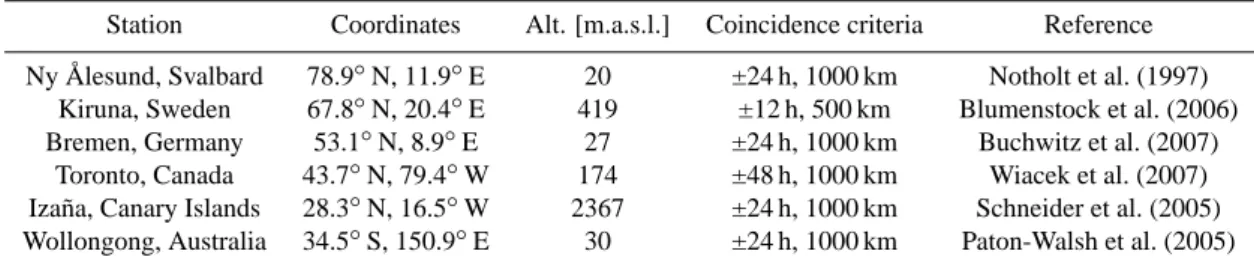
Table 1 lists the stations that participated, their locations and the coincidence criteria used. Toronto and Wollongong
Table 1. List of the FTIR stations that provided data for the analyses (Sect. 5.3 and Sect. 6.3). The latitude and longitude of each station
are provided, together with the altitude above sea level in meters (m.a.s.l.). The coincidence criteria used in this study are indicated for each station in column 4. References describing the stations, measurements and analyses are given in column 5.
Station Coordinates Alt. [m.a.s.l.] Coincidence criteria Reference Ny ˚Alesund, Svalbard 78.9◦N, 11.9◦E 20 ±24 h, 1000 km Notholt et al. (1997)
Kiruna, Sweden 67.8◦N, 20.4◦E 419 ±12 h, 500 km Blumenstock et al. (2006) Bremen, Germany 53.1◦N, 8.9◦E 27 ±24 h, 1000 km Buchwitz et al. (2007)
Toronto, Canada 43.7◦N, 79.4◦W 174 ±48 h, 1000 km Wiacek et al. (2007) Iza˜na, Canary Islands 28.3◦N, 16.5◦W 2367 ±24 h, 1000 km Schneider et al. (2005) Wollongong, Australia 34.5◦S, 150.9◦E 30 ±24 h, 1000 km Paton-Walsh et al. (2005)
use Bomem DA8 FTIRs with resolutions of 0.004 cm−1and
optical path differences of 250 cm, whereas the other
sta-tions use Bruker FTIRs (Ny ˚Alesund and Kiruna: 120 HR,
Bremen: 125 HR and Iza˜na: 120 M until end of 2004, then 125 HR). All Bruker instruments have a resolution of
0.004 cm−1, but those shown here normally use 0.005 cm−1
for better signal-to-noise ratio. More information about the instruments, the retrieval methodologies and the measure-ments made at each of these sites can be found in the ref-erences provided in Table 1. The participating stations cover
latitudes from 34.5◦S to 78.9◦N, and provide measurements
from the subtropics to the polar regions in the Northern Hemisphere (see Fig. 5). There is only one station for which we have measurements in the Southern Hemisphere. Days for which coincident FTIR data were available for compari-son with ACE are as follows:
– Ny ˚Alesund: NO2: 23 and 28 September 2004, 14 and
16 March 2005, 26 September 2005; NO: 14 and 16 March 2005.
– Kiruna: NO2: 27 and 29 October 2004, 25
Jan-uary 2005, 1, 2 and 7 FebrJan-uary 2005, 18, 19, 23 and 25 May 2005, 5 February 2006, 20 March 2006, 18 May 2006; NO: 27 and 29 October 2004, 7 February 2005, 18, 19 and 25 May 2005, 10 November 2005, 5 February 2006, 18 May 2006.
– Bremen: NO2: 2 and 3 September 2004, 24 March
2005, 13 February 2006, 8, 9 and 12 May 2006, 3, 25, 26 and 27 July 2006, 28 November 2006.
– Toronto: NO2: 23 and 29 July 2004, 2 June 2005, 1 and
2 September 2005, 3 and 5 May 2006, 31 August 2006; NO: 23 and 29 July 2004, 29 July 2005, 3 May 2006, 29 July 2006, 31 August 2006.
– Iza˜na: NO2: 5 and 30 April 2005, 1, 2 and 30 August
2005 and 20 October 2005; NO: 3 August 2004, 5 and 30 April 2005, 1, 2 and 30 August 2005.
– Wollongong: NO2: 1 March 2005, 3 November 2005,
20 and 21 August 2006, 31 October 2006 and 1
Novem-ber 2006; NO: 3 and 4 OctoNovem-ber 2004, 1 March 2005, 19 April 2005, 20 and 21 August 2006, 31 October 2006 and 1 November 2006.
The FTIR measurements require clear-sky conditions and
take measurements all year round during daylight. Only
cloud-free measurements are included in the comparisons. The data used here were analyzed using either the SFIT2 retrieval code (Pougatchev and Rinsland, 1995; Pougatchev et al., 1995; Rinsland et al., 1998) or PROFFIT92 (Hase,
2000). Both algorithms employ the optimal estimation
method (Rodgers, 2000) to retrieve vertical profiles from a statistical weighting between a priori information and the high-resolution spectral measurements. The retrieval codes have been compared and it was found that the differences were less than ∼1% (Hase et al., 2004). Averaging kernels calculated as part of this analysis quantify the information content of the retrievals, and can be used to smooth the ACE profiles, which have higher vertical resolution.
For NO2, there are typically 0.1 to 2 Degrees Of
Free-dom for Signal (DOFS, equal to the trace of the averaging kernel matrix) and for NO about one DOFS is found in the altitude range coincident with ACE-FTS measurements and about half a DOFS greater for the total columns.
Given this coarse vertical resolution, we compare partial columns rather than profiles. All sites used spectroscopic data from HITRAN 2004, with the exception of Kiruna and
Iza˜na (HITRAN 1996 for NO2and HITRAN 2001 for NO).
Comparisons of FTIR retrievals using HITRAN 1996 and
2004 showed that NO2 total and partial columns are about
2% lower when using HITRAN 1996.
Other information required for the retrievals, such as a pri-ori profiles and covariances, treatment of instrument line-shape, and atmospheric temperature and pressure are opti-mized for each site as appropriate for the local conditions.
4 Validation approach
4.1 Comparison methodology
The comparisons shown in this work use ACE data from 21 February 2004 (the start of the ACE Science Operations phase) through to 28 March 2007. The coincidence criteria needed to search for correlative measurements were deter-mined by considering temporal and spatial variability. The statistical significance of the results for the satellite compar-isons was also considered. Ground-based and balloon surements were considered coincident with the ACE mea-surements when they were within 1000 km and 24 h of each other. This resulted in cases, notably for balloon compar-isons, where only one ACE coincidence profile was avail-able. The value that was used in searching for coincidences is the location for each ACE occultation, which is defined as the latitude, longitude and time of the tangent point at 30 km (calculated geometrically). We do not expect a seasonal bias with solar occultation instruments, therefore seasonal depen-dencies were not studied here.
Because NO2 and NO are short-lived species, a
chemi-cal box model (described in Sect. 4.2) was used for all but the solar occultation comparisons and the MIPAS-IMK/IAA
NOxcomparisons, to correct for the time difference in
satel-lite comparisons. For the ground-based, aircraft and bal-loon measurements, box model scaling was applied when the measurements were not taken at the same solar zenith angle. For the balloon measurements, profiles obtained within 36 h and 1000 km of ACE were used. For the FTIR compar-isons, measurements that occurred within 24 h and 1000 km of ACE occultations were compared, with the exception of Kiruna where tighter criteria (12 h and 500 km) were used. These relaxed criteria were necessary to obtain a reasonable number of ACE coincidences for each station (between 5 and 72). In cases where several FTIR measurements from a site were available for one ACE occultation or vice versa, all pairs were considered.
Table 1 lists the FTIR stations and Table 2 summarizes all other correlative data sets, comparison periods, temporal and spatial coincidence criteria, and number of coincidences.
The satellite VMR profiles and the SAOZ-balloon VMR profiles all have vertical resolutions that are similar to those of the ACE instruments, and so no averaging kernel smooth-ing was applied to these data. These correlative profiles were linearly interpolated on to the 1-km ACE-FTS or the 0.5-km MAESTRO altitude grid. The balloon-borne SPIRALE VMR profile was obtained at significantly higher vertical resolution than the ACE instruments, and so was convolved with a triangular function having full width at the base equal to 3 km and centered at the tangent heights of each occul-tation for ACE-FTS and with a Gaussian function having full width at half maximum equal to 1.7 km for MAESTRO. This approach simulates the smoothing effect of the limited resolution of the ACE instruments, as discussed by Dupuy
et al. (2008). The resulting smoothed profiles were then interpolated onto the 1-km grid for ACE-FTS and the 0.5-km grid for MAESTRO. Finally, for the comparisons with the ground-based FTIR and UV-VIS measurements, which have significantly lower vertical resolution, the ACE profiles were smoothed by the appropriate FTIR or UV-VIS aver-aging kernels to account for the different vertical sensitiv-ities of the two measurement techniques. The method of Rodgers and Connor (2003) was followed and Eq. (4) from their paper was applied, using the a priori profile and the av-eraging kernel matrix of the FTIR and the UV-VIS instru-ments (see Sect. 5.3). Partial columns over specified altitude ranges were then calculated for the ACE instruments and the FTIRs or the UV-VIS instruments and used in the compar-isons. Additionally, the UV-VIS profiles were compared to the smoothed profiles from the ACE instruments.
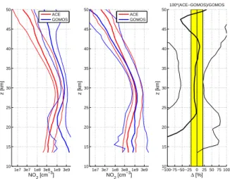
Pairs of vertical VMR profiles from ACE (both FTS and MAESTRO) and each validation experiment (referred to as VAL in text and figures below) were identified using the ap-propriate temporal and spatial coincidence criteria. The re-sults of the vertical profile comparisons will be shown be-low, with some modifications for the GOMOS comparisons (Sect. 5.1.3), the single profile comparisons (SPIRALE and SAOZ; Sect. 5.2) and the FTIR and UV-VIS partial column comparisons (Sects. 5.3 and 5.4).
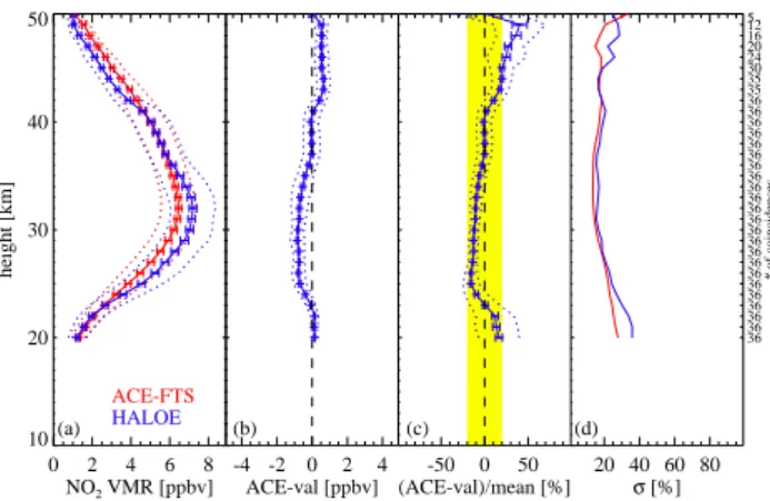
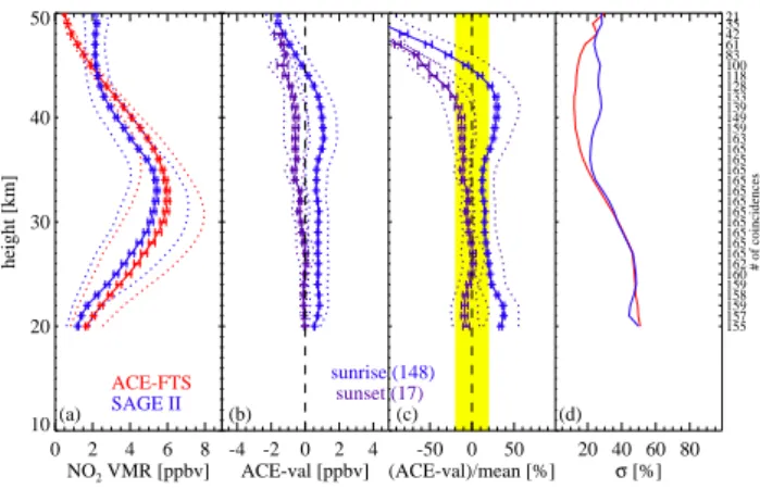
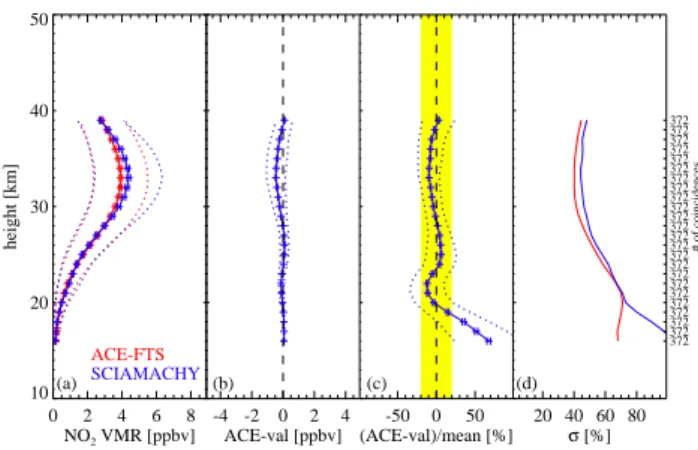
(a) The mean profile of the ensemble for ACE and the mean profile for VAL are plotted as solid lines with the stan-dard deviations on each of these two profiles, ±1σ , as dotted lines, in panel (a) of the comparison figures discussed below. The uncertainty in the mean is calculated as σ (z)/
√ N (z)
(where N (z) is the number of points used to calculate the mean at a particular altitude) and is included as error bars on the lines in panel (a). Note: in some cases, these error bars, as well as those in panels (b) and (c) (see below) may be small and difficult to distinguish.
(b) The mean profile of the absolute differences, ACE−VAL is plotted as a solid line in panel (b) of the com-parison figures below, and the standard deviation in the distri-bution of this mean difference, ±1σ as dotted lines. The term absolute here refers to differences of the compared VMR val-ues and not to absolute valval-ues in the mathematical sense. The differences are calculated for each pair of profiles at each al-titude, and then averaged to obtain the mean absolute differ-ence at altitude z: 1abs(z)= 1 N (z) N (z) X i=1 [ACEi(z) −VALi(z)] (1)
where N (z) is the number of coincidences at z, ACEi(z)is
the ACE (FTS or MAESTRO) VMR at z for the ith
coin-cident pair, and VALi(z)is the corresponding VMR for the
validation instrument. Error bars are also included in these figures. For the statistical comparisons involving multiple coincidence pairs (the satellite and UV-VIS profile compar-isons), these error bars represent the uncertainty in the mean.
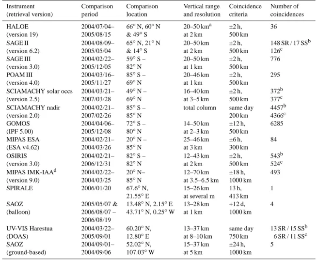
Table 2. Summary of the correlative data sets for the instruments used in the statistical and individual profile comparisons with ACE-FTS
and MAESTRO NO2and ACE-FTS NO. All values are for NO2comparisons unless noted for NO or NOx, SR is sunrise and SS is sunset. Instrument Comparison Comparison Vertical range Coincidence Number of
(retrieval version) period location and resolution criteria coincidences
HALOE 2004/07/04– 66◦N, 60◦N 20–50 kma ±2 h, 36 (version 19) 2005/08/15 & 49◦S at 2 km 500 km SAGE II 2004/08/09– 65◦N, 21◦N 20–50 km ±2 h, 148 SR / 17 SSb (version 6.2) 2005/05/04 & 14◦S at 2 km 500 km 126c SAGE III 2004/02/22– 59◦S – 20–50 km ±2 h, 776 (version 3.0) 2005/12/05 82◦N at 1 km 500 km POAM III 2004/03/16– 85◦S – 20–46 km ±2 h, 295 (version 4.0) 2005/11/27 69◦N at 1 km 500 km
SCIAMACHY solar occs 2004/03/21– 49◦N – 16–40 km ±2 h, 372b
(version 2.5) 2007/03/28 69◦N at 3–5 km 500 km 377c
SCIAMACHY nadir 2004/02/21– 85◦S – total column same day 4457b
(version 2.0) 2007/02/26 85◦N 200 km 4366c GOMOS 2004/04/06– 72◦S – 14–50 km ±12 h, 6285 (IPF 5.00) 2005/12/08 80◦N at 2–3 km 500 km MIPAS ESA 2004/02/21– 20◦N – 25–46 km ±6 h, 84 (ESA v4.62) 2004/03/26 85◦N at 3 km 300 km OSIRIS 2004/02/21– 82◦S – 12–43 km ±2 h, 543b (version 3.0) 2006/12/31 82◦N at 2 km 500 km 524c MIPAS IMK-IAAd 2004/02/22– 20◦N– 12–70 km ±18 h, 493 (version 9.0) 2004/03/25 85◦N at 3.5–6.5 km 1000 km SPIRALE 2006/01/20 67.6◦N, 15–26 km 13 h, 1 21.55◦E at several m 413 km SAOZ 2005/05/07 & 13.48◦N, 2.15◦E 13–28 km +12 d, 4 (balloon) 2006/08/07 – 43.71◦N, 0.25◦W at 1 km 1000 km 2006/08/19
UV-VIS Harestua 2004/03/22– 60.20◦N, 13–37 km same day 13 SR / 15 SSb
(DOAS) 2005/09/01 12.80◦E at 8–10 km 750 km 6 SR / 11 SSc
SAOZ 2004/09/01– 52.02◦N, 15–37 km ±24 h, 5
(ground-based) 2004/09/06 107.03◦W at 5 km 1000 km
aValue given for NO
2comparisons. For the ACE-FTS comparison with NO, 20 to 108 km was used. bNumber of coincidences for ACE-FTS.
cNumber of coincidences for MAESTRO. dComparisons with NO
xfrom ACE-FTS only.
(c) Panel (c) of the comparison figures presents the mean profile of the relative differences. This mean relative differ-ence is defined, as a percentage, using:
1rel(z) =100% × 1 N (z) N (z) X i=1 ACEi(z) −VALi(z) MEANi(z) (2)
where MEANi(z) = [ACEi(z) +VALi(z)]/2 is the mean of
the two coincident profiles at z for the ith coincident pair. (d) The relative standard deviations on each of the ACE and VAL mean profiles calculated in step (a) are given in panel (d), with the number of coincident pairs given as a function of altitude on the right-hand y-axis for the statistical comparisons.
For single profile comparisons (SPIRALE, SAOZ), error bars represent the combined random error for all panels. The
ACE-FTS data products include only statistical fitting errors, while MAESTRO provides an estimate of relative uncertain-ties (as described in Sect. 2). No systematic errors are avail-able, therefore the error bars for the single profile compar-isons are very small. They cannot be compared directly with the total errors of the single profile instruments.
4.2 Diurnal mapping using a chemical box model
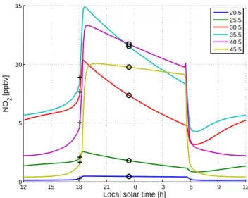
In Fig. 6, we present a typical example of the modelled
tem-poral evolution of the NO2 concentration in the equatorial
region together with the ACE-FTS and GOMOS local so-lar time at six different altitudes using the photochemical box model described by Prather (1997) and McLinden et al. (2000). This highlights an obstacle faced in the validation of species that experience diurnal variations when there are
mismatches between the local time of the primary measure-ment and that of the correlative measuremeasure-ment. Since diur-nal gradients are generally largest through sunrise and sun-set, this is even more problematic for comparisons involving solar occultation instruments such as ACE-FTS and MAE-STRO. The approach adopted in this paper is to simply scale,
or map, the profile from the local time, t1, of one instrument
to the local time, t2, of another instrument. The diurnal
scal-ing factors, st, were computed in a photochemical box model
as follows:
st(z) =
VMRmodel(t2, z)
VMRmodel(t1, z)
, (3)
where VMRmodel is the modelled VMR and z represents the
vertical co-ordinate (altitude, pressure or potential
tempera-ture). Then the VMR at local time, t2, can be calculated from
the VMR at local time t1using
VMR(t2, z) = st(z) ×VMR(t1, z). (4)
This approach was successfully applied in the validation
of OSIRIS NO2observations, in which diurnal scaling
fac-tor look-up tables, based on climatological ozone and tem-perature, were employed to enable comparisons with solar occultation instruments (Brohede et al., 2007a). A recent improvement is the calculation of scaling factors for each profile, using simultaneous observations of ozone, temper-ature, and pressure to help constrain the diurnal cycle (Bro-hede et al., 2007b). Similar approaches have been used else-where (Bracher et al., 2005b).
Following this method, diurnal scaling factors have been pre-calculated for each ACE occultation using the Univer-sity of California at Irvine (UCI) photochemical box model (Prather, 1997; McLinden et al., 2000). Each simulation is constrained with the ACE-FTS version 2.2 retrieved temper-ature, pressure, and ozone (with updates). Other model
in-put fields include NOy and N2O from a three-dimensional
model (Olsen et al., 2001), Cly and Bry from tracer-tracer
correlations with N2O (Salawitch, personal communication,
2004), and background aerosol surface area from SAGE II (climatology data). Photochemical rate data was taken from Sander et al. (2003) and a surface albedo of 0.2 is assumed. Uncertainties introduced into the diurnally shifted profile are expected to be small, generally less than 10% in the middle stratosphere and 20% in the lower/upper stratosphere (Bro-hede et al., 2007b).
Beyond the local time issue, there is the more subtle prob-lem of the so-called diurnal effect (Newchurch et al., 1996; McLinden et al., 2006). The diurnal effect arises when a range of solar zenith angles are sampled along the line-of-sight and systematic errors in species that experience
diur-nal variations (such as NO and NO2) may result. The sign
and magnitude of the error are governed by the gradients of the species through the effective range in solar zenith angle
sampled (roughly 85 to 95◦for solar occultations) (McLinden
et al., 2006). For solar occultation measurements below 20
12 15 18 21 0 3 6 9 12
0 5 10 15
Local solar time [h]
NO 2 [ppbv] 20.5 25.5 30.5 35.5 40.5 45.5
Fig. 6. Modelled time evolution of the NO2concentration at
dif-ferent altitudes in the equatorial region (ACE sunset for orbit 3491: 9.0◦N, 64.6◦E; GOMOS: 7.7◦N, 60.6◦E). Crosses and circles re-fer to ACE and GOMOS local solar times, respectively.
to 25 km, NO2will be biased high by up to 50% and NO will
be biased low by as much as a factor of 2 to 4 if the diurnal effect is not accounted for in the retrieval, as is the case for the ACE instruments. The diurnal effect has a much smaller impact above about 25 km due to a near complete
cancella-tion of the near (SZAs greater than 90◦) and far (SZAs less
than 90◦) side biases.
A straightforward, yet representative method of estimat-ing these so-called diurnal effect errors for occultation has
been developed by McLinden (2008)2. In some
compar-isons, the diurnal effect has been forward modelled and a correction has been applied to the ACE measurements. For comparisons with OSIRIS (a limb-scatter instrument, which is subject to its own, analogous diurnal effect errors) an anal-ogous correction has been applied (McLinden et al., 2006; Brohede et al., 2007a). Note that for comparisons with most other solar occultation instuments, no correction is necessary as the effect will manifest equally. The exception to this is HALOE, which is corrected for the diurnal effect (Gordley et al., 1996).
2McLinden, C. A.: Diurnal effects in solar occultation observa-tions: error estimate and application to ACE-OSIRIS NO2 compar-isons, in preparation, 2008.
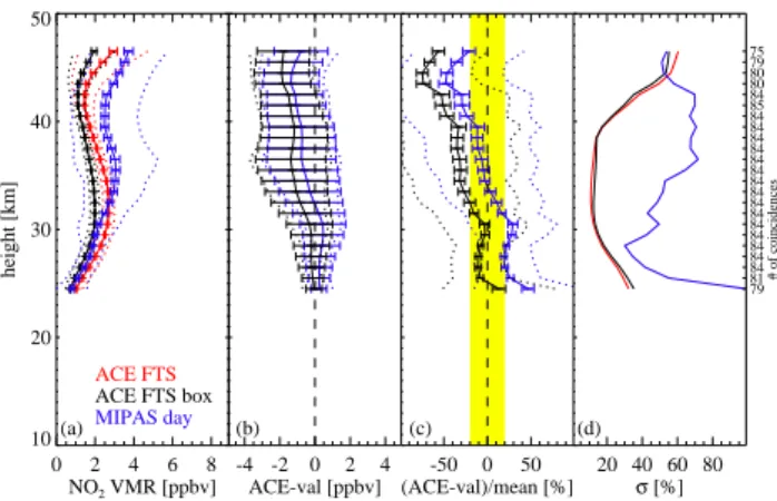
0 2 4 6 8 NO2 VMR [ppbv] 10 20 30 40 50 height [km] ACE-FTS MAESTRO (a) -4 -2 0 2 4 FTS-MAE [ppbv] (b) -50 0 50 (FTS-MAE)/mean [%] -50 0 50 (FTS-MAE)/mean [%] (c) 20 40 60 80 σ [%] (d) 7838 7842 7847 7849 7850 7847 7825 7817 7802 7788 7760 7738 7713 7692 7660 7623 7591 7528 7425 7251 6982 6646 6186 5645 5058 4384 3649 2942 2292 1693 1183 # of coincidences
Fig. 7. (a) Mean profiles for all measurements by ACE-FTS (solid
red) and MAESTRO (solid black) from 21 February 2004 to 31 De-cember 2006. Dotted lines are the profiles of standard deviations (σ ) of the distributions, while error bars (often too small to be seen) represent the uncertainty in the mean (σ/
√
N). (b) Mean abso-lute differences between ACE-FTS and MAESTRO (solid). Dot-ted lines represent the standard deviation of the distribution of the differences while error bars represent the uncertainty in the mean difference. (c) Mean percent differences (solid) between ACE-FTS and MAESTRO relative to the mean of the two instruments, for all coincidences. Dotted lines represent the standard deviation of the distribution of the differences while error bars represent the uncer-tainty in the mean difference. The range from ±20% is highlighted in yellow. (d) Standard deviations of the distributions (σ ) relative to the mean VMR of each instrument at each altitude, for all co-incident events, for ACE-FTS (red) and MAESTRO (black). The number of the coincidences is indicated on the right-hand y-axis.
0 2 4 6 8 10
MAESTRO NO2 partial column [10 15 cm-2 ] 0 2 4 6 8 10 ACE-FTS NO 2 partial column [10 15 cm -2] ACE-FTS = 0.92 MAESTRO - 0.03 r = 0.96
Fig. 8. Scatter plot of the ACE-FTS and the MAESTRO NO2
par-tial columns (14.5 to 46.5 km). Data shown is used for the SCIA-MACHY nadir comparisons (Sect. 5.1.6). The solid red line is the linear least-squares fit to the data, with the slope, intercept, and cor-relation coefficient given in the figure. The dashed black line shows the one-to-one linear relationship for comparison.
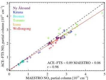
0 1 2 3 4 5
MAESTRO NO2 partial column [10
15 cm−2] 0 1 2 3 4 5 ACE−FTS NO 2 partial column [10 15 cm −2] Ny Ålesund Kiruna Bremen Toronto Izana Wollongong ACE−FTS = 0.89 MAESTRO + 0.06 r = 0.98
Fig. 9. Scatter plot of the ACE-FTS and MAESTRO NO2partial
columns (data shown is used in the FTIR comparisons in Sect. 5.3) at the times of the FTIR comparisons. The red line is the linear least-squares fit to the data, with the slope, intercept, and correlation coefficient given in the figure. The dashed black line shows the one-to-one line relationship for comparison. The colours indicate the NDACC stations for which coincident measurements exist. The partial columns were calculated over different altitude ranges for each station (see Table 3). ACE-FTS and MAESTRO VMRs have been photochemically corrected to the times of the ground-based measurements.
5 Results for the NO2comparisons
5.1 Satellites
5.1.1 ACE-FTS and MAESTRO NO2
Because they share a single suntracker and have aligned fields-of-view, ACE-FTS and MAESTRO measure the same
air mass at the same time and place. Comparisons of NO2
measurements from these two instruments have been done previously by Kerzenmacher et al. (2005) for ACE-FTS ver-sion 1.0 and preliminary MAESTRO data, for which agree-ment of 40% was found with a very small data set, and by Kar et al. (2007) for one year of the current data sets. Kar et al. (2007) found good agreement (within 10 to 15% from 15 to 40 km) for sunrise measurements and similar agreement for the sunset measurements (within 10 to 15% from 22 to 35 km). In Fig. 7, a comparison of all MAESTRO and
ACE-FTS NO2measurements is shown (from 21 February 2004 to
31 December 2006). It can be seen that the differences are in very good agreement with Kar et al. (2007): the ACE-FTS and MAESTRO measurements agree to within 10% from 23
to 40 km. Up to 35 km, ACE-FTS measures less NO2 than
MAESTRO. MAESTRO VMRs are lower at higher altitudes, with differences reaching values of 50% at 45 km.
There are some altitudes (38 to 41 km and 47 to 50 km) where the absolute differences are negative but the rela-tive differences are posirela-tive. This is most obvious near 47